E
SSAYS ONC
REDITM
ARKETD
EVELOPMENT ANDL
ABORM
ARKETC
HOICESAlina Malkova
A dissertation submitted to the faculty of the University of North Carolina at Chapel Hill in par-tial fulfillment of the requirements for the degree of Doctor of Philosophy in the Department of
Economics.
Chapel Hill 2020
Approved by:
Klara Peter
Luca Flabbi
David Guilkey
Andr´es Hincapi´e
c
2020
ABSTRACT
ALINA MALKOVA: Essays on Credit Market Development and Labor Market Choices. (Under the direction of Klara Peter)
My dissertation is a series of papers examining the link between the credit market accessibility
(CMA) and individual labor market decisions.
The first chapter analyzes a decline in the ability to obtain financing as a potential explanation
for the observed decrease in the U.S. self-employment. The shrinking of the U.S. bank branch
network since 2010 and the increased average borrower-lender distance reduce the accessibility of
credit institutions for borrowers. To evaluate the impact of the CMA on entry into self-employment,
I disaggregate the self-employed into two categories: entrepreneurs whose businesses depend on
business loans (Type-1) and other self-employed (Type-2). Using a novel data source (the
Commu-nity Advantage Panel Survey database), I find that the proximity of credit market institutions has
heterogeneous effects on transition to self-employment. An improvement in the CMA increases
the likelihood of transition to Type-1 self-employment. But for the Type-2 self-employed, the
effect is the opposite: the probability of transition to Type-2 employment decreases and
self-employed workers of this type are more likely to switch to paid employment to be able to receive
non-business related loans. The chapter discusses the implications of these results for different
policies.
The second chapter investigates the effects of the credit market development on the labor
mo-bility between the informal and formal labor sectors. In the case of Russia, due to the absence
of a credit score system, a formal lender may set a credit limit based on the verified amount of
income. To get a loan, an informal worker must first formalize his or her income (switch to a
formal job), and then apply for a loan. To show this mechanism, the RLMS data was utilized,
and the empirical method is the dynamic multinomial logit model of employment. The empirical
informal to a formal job, and improved CMA (by one standard deviation) increases the chances of
informal sector workers to formalize by 5.4 ppt. These results are robust in different specifications
of the model. Policy simulations show strong support for a reduction in informal employment in
ACKNOWLEDGMENTS
I would like to thank Klara Peter, Luca Flabbi, David Guilkey, Andr´es Hincapi´e, and Helen
Tauchen for serving on my thesis committee and providing valuable guidance and feedback. I
am grateful for discussions with many people, including Donna Gilleskie, Jane Fruehwirth, Qing
Gong, Siddhartha Biswas, Mauricio Salazar, Ray Wang, and participants of the Applied Micro
seminar at the University of North Carolina at Chapel Hill. I deeply appreciate Andrey Minaev for
helpful comments and support. I gratefully acknowledge the Center of Community Capital UNC,
the Ford Foundation and Sarah Riley for providing access to the CAPS database, helpful feedback,
TABLE OF CONTENTS
LIST OF TABLES . . . ix
LIST OF FIGURES . . . xi
1 Knockin’ on the Bank’s Door: Why is Self-Employment Going Down? . . . 1
1.1 Introduction . . . 1
1.2 Related Literature . . . 5
1.3 Testable Implications of Theoretical Model . . . 8
1.4 Empirical Model and Identification . . . 10
1.4.1 The Timeline of the Model . . . 10
1.4.2 Dynamic Multinomial Logit Model of Employment . . . 10
1.4.3 Identification . . . 12
1.5 Data . . . 15
1.5.1 Sources of Data . . . 15
1.5.2 Explanatory Variables . . . 17
1.5.3 Constructed Variables . . . 18
1.6.1 Access to Credit Products . . . 21
1.6.2 Results of the Main Model . . . 22
1.6.3 Robustness Analysis . . . 25
1.7 Conclusion . . . 27
1.8 Figures . . . 29
1.9 Tables . . . 33
2 Labor Informality and Credit Market Development . . . 44
2.1 Introduction . . . 44
2.2 Literature Review . . . 46
2.3 Theoretical model . . . 50
2.3.1 Setup . . . 50
2.3.2 Borrowing Constraints . . . 52
2.4 The Dynamics of Informality and Local Credit Market . . . 53
2.4.1 Timeline of the Model . . . 53
2.4.2 Dynamic Multinomial Logit Model of Employment . . . 54
2.4.3 Credit Market and Employment Transitions . . . 57
2.5 Data . . . 59
2.5.1 Employment Status,Yijt . . . 59
2.5.3 Exclusion Restrictions for Initial Conditions,Ri1 . . . 62
2.5.4 Estimation Sample and Summary Statistics . . . 62
2.5.5 Credit Market Participation and Local Credit Accessibility . . . 63
2.6 Results . . . 67
2.6.1 Probability of Transition to the Formal Sector . . . 67
2.6.2 Results of the Main Model . . . 68
2.6.3 Robustness Analysis . . . 70
2.6.4 Policy Simulations . . . 74
2.6.5 Effect of Credit Market Accessibility on Informal Sector . . . 75
2.6.6 Loan Equation . . . 75
2.7 Conclusions . . . 77
2.8 Figures . . . 79
2.9 Tables . . . 85
A Appendix to Chapter 2 . . . 99
A.1 Variables . . . 99
A.2 Supplementary Tables . . . 103
LIST OF TABLES
1.1 Alternative Definitions of Types of Self-Employment . . . 20
1.2 Summary Statistics . . . 33
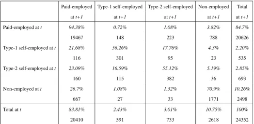
1.3 Transition Matrix between Labor Markets. Definition Based on Type of Business: Incorporated/Unincorporated . . . 34
1.4 Random-Effects Probit Model of Access to Credit . . . 35
1.5 Dynamic Multinomial Logit Model of Employment Choices. The types of self-employment are based on the legal status of the business (main specification) . . . 36
1.6 Post-estimation predictions: Average marginal effect of CMA on transition proba-bility . . . 39
1.7 Results of Dynamic Multinomial Logit Model of Employment Choices for Differ-ent Definitions of Types of Self-employmDiffer-ent . . . 41
1.8 Results of Dynamic Multinomial Logit Model of Employment Choices for Differ-ent IdDiffer-entifying Assumptions . . . 42
1.9 Results of Dynamic Multinomial Logit Model of Employment Choices with En-dogenous CMA . . . 43
2.1 Trends in Employment Status . . . 85
2.2 Sample Selection Criteria . . . 86
2.3 Sample Selection Criteria . . . 87
2.5 Dynamic Multinomial Logit Model of Employment Choice . . . 90
2.6 Post-estimation predictions: Average marginal effect ofCit . . . 92
2.7 Robustness Analysis of the Dynamic Employment Model with Unobserved
Het-erogeneity . . . 93
2.8 Dynamic Employment Model with Disaggregated Groups of Informal Workers . . 94
2.9 Post-estimation predictions: Average marginal effect ofCit on transition probability 95
2.10 Predicted Probabilities from Simulated Policies . . . 96
2.11 Heterogeneous Effects of Credit Market Accessibility on the Informal Sector . . . 97
2.12 Heterogeneous Effects of Credit Market Accessibility on the Informal Sector . . . 98
A.1 Dynamic Multinomial Logit Model of Employment Choice . . . 103
A.2 Dynamic Multinomial Logit Model of Employment Choice . . . 104
A.3 Dynamic Employment Model Based with the Categories of Informal Pay . . . 105
A.4 Post-estimation predictions: Average marginal effect ofCiton transition
probabil-ity . . . 106
A.5 Different Measures of Credit Market Accessibility . . . 107
LIST OF FIGURES
1.1 Number of the Unincorporated Self-Employed in the U.S. . . 29
1.2 Self-Employment Rate in the U.S. . . 29
1.3 Average Minimum Borrower-Lender Distance . . . 30
1.4 Credit Market Accessibility Index . . . 30
1.5 Location of All Banks in the U.S. . . 31
1.6 Location of All Banks in the U.S. and the Hot Spot Analysis . . . 31
1.7 Marginal Effects of CMA on Predicted Probability of Being Self-Employed . . . . 40
1.8 Marginal Effects of CMA on Predicted Probability of Being Self-Employed . . . . 40
2.1 Timeline . . . 79
2.2 Share of Loan-Taking Households . . . 80
2.3 Distance to the Nearest Bank Office . . . 81
2.4 Measure of formal credit market accessibility . . . 82
CHAPTER 1
KNOCKIN’ ON THE BANK’S DOOR: WHY IS SELF-EMPLOYMENT GOING DOWN?
1.1 Introduction
The self-employed sector in the U.S. has lost almost 1 million workers since 19941(see Figure
1.1). The share of the self-employed in total employment decreased from 12.1 percent in 1994 to
10.1 percent in 2015 (Hipple 2016)2. The literature provides limited reasoning for the decrease
in the number of the self-employed. According to Hipple (2016), the decline in self-employment
may be associated with a decline in agricultural employment. Another reason for this decline is
documented by Schweitzer and Shane (2016). The authors find that business cycles affect
transi-tions in and out of self-employment3, while the recent fall in the aggregate demand explains the
exit from entrepreneurship. This paper focuses on the decline in the ability to obtain financing as
another potential explanation for the observed trends in self-employment.
In recent years, two factors may have contributed to the lower credit market accessibility
(CMA) for the self-employed. The de-liberalization of the financial system during the Great
Re-cession resulted in enhanced regulatory scrutiny and tighter collateral requirements for borrowers
1 The number is reported by the U.S. Bureau of Labor Statistics (BLS) as the number of unincorporated self-employed persons. The definition of self-self-employed individuals also comes from BLS. Self-self-employed people are those who work for profit or fees in their own business, profession, trade, or farm, including those who intended to earn a profit but whose business produced no profit or a loss. Unless otherwise specified, the Current Population Survey (CPS) estimates of the self-employed published by BLS reflect only people whose businesses are unincorporated. BLS classifies the incorporated self-employed as wage and salary workers, because the incorporated self-employed are paid employees of their corporations.
2 From 1994 to 2015, the unincorporated self-employment rate fell from 8.7 percent to 6.4 percent. From 1994 to 1999, the share of total employment made up of the incorporated self-employed ranged from 3.2 percent to 3.5 percent. Over the 2000-08 period, the incorporated self-employment rate rose from 3.3 percent to 4.0 percent. The rate then edged down to 3.7 percent in 2010 and remained at that level over the 2011-15 period (see Figure 1.2).
(Wiersch and Shane 2013). But the recovery of the financial system and the easing of
require-ments for borrowers did not lead to the pre-crisis levels of self-employment. The other factor is
the shrinking of the U.S. bank branch network since 2010 and, as a consequence, the increased
average borrower-lender distance (see Figure 1.3) (Nguyen 2019). The Federal Deposit Insurance
Company (FDIC) claims that at least 80 percent of branch closings should not have any
mean-ingful impact on the physical access to banks, as they occur in areas with multiple remaining
branches4However, the borrowing process for the self-employed is informationally intensive, and
credit approvals primarily rely on soft information about the borrower (DeYoung, Glennon, and
Nigro 2008). In other words, personal presence during a loan transaction can still play an essential
role in obtaining financing.
This study confirms that the CMA declined substantially in the U.S. between 2007 and 2014
(see Figure 1.4). In this context, the accessibility is proxied by the average borrower-lender
dis-tance, the number of nearby branches, and the number of bank employees in the county of
resi-dence. However, the effect of the reduced physical CMA on self-employment rates is ambiguous.
On the one hand, the relationship between the CMA and the probability of being self-employed
could be positive. A few previous studies find that a shorter lender-borrower distance increases
business lending (Nguyen (2019); Degryse and Ongena (2005)), which may positively influence
the number of entrepreneurs. On the other hand, studies from countries with a large informal
sec-tor show that new bank openings create incentives for individuals working in the informal secsec-tor
to switch to jobs with verifiable income in order to be eligible for loans and thus transfer to paid
employment (Malkova et al. 2019). In the case of the U.S., a shorter borrower-lender distance may
create incentives for self-employed workers with restricted access to the credit market5 to switch
4 Branch closings are heavily regulated by the FDIC (https://www.fdic.gov/regulations/laws/ rules/5000-3830.html). 4 Before closing a branch, banks must provide detailed research and statistics about the effect of the closure on the local economy, and clients must receive a notice 90 days prior to the branch closing in a given area.
to paid employment to be able to use credit products. In other words, the effect of the CMA on
transition to self-employment is likely to be heterogeneous, which is the focus of this study.
The study utilizes several sources of U.S. data between 2003 and 2014. The main database is
the Community Advantage Panel Survey (CAPS)6database. The benefit of using this database is
the opportunity to identify geographical distances between each individual and all banks within
the state. The location of banks is taken from the FDIC Summary of Deposits (SOD) data7. To
diminish the effect of the unobservable local economic conditions that are correlated with the credit
supply, I also use county and tract-level control variables from the American Community Survey
(ACS).
The paper proceeds in two parts. In the first part, I discuss testable implications from an
intuitive theoretical model (a three-sector Roy model) that shows the effect of the CMA on the
labor mobility among three labor states: two types of self-employment (SE) and paid employment
(wage employment). The theoretical model is based on the works by Evans and Jovanovic (1989)
and Levine and Rubinstein (2018). To show the heterogeneous effects of the CMA on decisions
to become self-employed, I divide self-employed workers into two types. The first one (Type-1
self-employed) includes entrepreneurs, owners of firms that demand physical capital and business
loans8. The second one (Type-2 self-employed) comprises non-entrepreneurs and owners of
com-panies without business loans; in other words, the agent uses own initial wealth to start a business.9
In the theoretical model, agents enter self-employment (Type-1 and Type-2) based on their
compar-ative advantage that depends on their abilities and the amount of available assets. Individuals face
6CAPS comprises 11 years of a panel survey of approximately 5,000 low- and moderate-income homeowners and renters during the period of 2003-2014. The data collection has been conducted by the UNC Center for Community Capital with generous funding from the Ford Foundation.
7FDIC SOD provides an annual enumeration of all branches belonging to FDIC-insured institutions. As of Septem-ber 2019, the FDIC provided deposit insurance at 5,256 institutions. The FDIC insures deposits in memSeptem-ber banks up to US$250,000 per ownership category.
8Among the Type-1 self-employed, mention may be made of computer programmers, lawyers, doctors, real estate managers, etc.
borrowing costs including both interest costs and non-interest costs (the time costs of arranging a
loan and any monetary initiation costs). The comparative static shows that lower non-interest costs
of borrowing (better CMA) increase the probability of being Type-1 self-employed, decrease the
probability of being Type-2 self-employed, and increase the probability of transition from Type-2
self-employment to paid employment.
The second part of the paper is an empirical analysis that aims to estimate the impact of the
CMA on transitions in and out of self-employment. The CMA is measured as an index based
on a combination of the following variables: the average distance from an individual to 10
near-est banks, the number of banks and branches within 5 miles from the individual, and the number
of bank workers per 1,000 population at the county level. The model used for this analysis is a
dynamic multinomial logit model of employment with correlated random effects. The empirical
challenge is that banks choose where to locate branches depending on the local economic
con-ditions that are correlated with the number of the self-employed in a given area. I use several
approaches to identify the causal effect of the CMA on decisions to become self-employed. First,
I control for the set of variables that proxy the local economic conditions at the county level: the
number of business establishments, the unemployment rate, the share of the population with
pro-fessional, scientific, management and administrative education. Second, I include in the model
the within-means of CMA characteristics that accounts for the endogeneity of the CMA with
re-gards to unobserved factors like the fixed-effect model. In addition, I estimate the model using
the exposure to post-merger consolidation of banks at the Census tract level as an instrument for
CMA changes (Nguyen (2019); Garmaise and Moskowitz (2006)). In this paper, I consider
merg-ers of large banks, defined as mergmerg-ers where both banks held at least US$1 billion in pre-merger
assets. The average Census tract is 1.5 square miles, and the decision of large banks to merge is
plausibly exogenous to the local economic conditions in a Census tract where both banks have a
branch. The merger-induced consolidation decreases competition between banks at the tract level,
which may be followed by a branch closure (Nguyen (2019)) and an increase in the
The empirical analysis shows heterogeneous effects of the CMA on transitions in and out of
self-employment depending on the type of self-employed workers. For the Type-1 self-employed, an
improvement of the CMA increases the probability of transition in self-employment. While for the
Type-2 self-employed, an improvement of the CMA increases the probability of transition out of
self-employment.
1.2 Related Literature
This paper connects two strands of literature. The first one examines how a decision to
be-come an entrepreneur is associated with access to capital, wealth, and collateral constraints. There
is an extensive literature focusing on the positive correlation between housing wealth and
en-trepreneurial activities (Fan and White (2003), Fairlie and Krashinsky (2012), Fort, Haltiwanger,
Jarmin, and Miranda (2013), Corradin and Popov (2015)). The literature shows that credit
con-straints at the household level matter for the creation of new businesses (Evans and Jovanovic
(1989), Holtz-Eakin, Joulfaian, and Rosen (1994), Gentry and Hubbard (2004), Cagetti and De Nardi
(2006)). Previous work has also found that a bank loan is an essential source of financing for small
businesses (Petersen and Rajan (1994), Bates and Robb (2013), Fracassi, Garmaise, Kogan, and
Natividad (2013)) and that entrepreneurs often have to provide personal guarantees when they
obtain financing (Berger and Udell (1998); Greenstone, Mas, and Nguyen (2014)).
Herkenhoff, Phillips, and Cohen-Cole (2016) examine how the access to consumer credit
im-pacts employment prospects, earnings, and entrepreneurship. To isolate the causal effect of credit
on labor market outcomes, authors use bankruptcy flag removals10 to separate a sizable discrete
increase in credit access. Authors show that following the flag removal there is: (a) an increased
flow rate into self-employment, (b) disproportionate borrowing by new self-employed entrants
rel-ative to other job transitioners, (c) an increased likelihood of starting an employer business, (d)
an increase in startups entering capital intensive and external finance intensive industries, and (e)
disproportionate borrowing by new employer businesses.
The second one is the growing strand of literature that studies the importance of the
geograph-ical distance for bank lending. Two broad channels have been identified in economics literature
for the effects of distance on credit market transactions. First, studies on spatial rationing have
established a correspondence between distance and credit rationing. A closer geographic distance
gives banks privileged access to soft information that facilitates the evaluation of the borrower’s
creditworthiness, thereby permitting them to gain a cost advantage for monitoring over more
re-mote competitors who may not enjoy the same degree of access to such information (Hauswald
and Marquez 2006). The information effect of distance has been shown empirically to facilitate ex
ante screening and ex post monitoring of borrowers in bank lending, giving well-informed banks
a competitive edge and market power (Petersen and Rajan (2002); Brevoort, Wolken, and Holmes
(2010); Guiso, Sapienza, and Zingales (2004); Sufi (2007); Qian and Strahan (2007)). One benefit
for borrowers located closer to their banks is that, with privileged access to information, inefficient
rationing might be reduced. Using a unique data set of all loan applications by small firms to a
large bank, Agarwal and Hauswald (2010) document that the closer a firm is to its branch office,
the more likely the bank is to offer credit. However, borrowing from closer banks is associated
with, for example, higher interest rates (Agarwal and Hauswald 2010). The reason is that
bor-rowers are informationally captured by lenders who have privileged access to soft information to
the extent that such information cannot be credibly communicated to outsiders (Dell’Ariccia and
Marquez 2004).
Second, a shorter lender-borrower distance potentially benefits both parties since it reduces
transaction costs. Examples of such costs for a potential borrower include transportation costs
incurred in the process of applying for a loan and the time and effort spent on either personally
interacting with loan officers or looking for a suitable loan. The reduction in the cost of obtaining
soft information for the lender is another benefit of the shorter distance. In classical models of
location differentiation (Salop 1979), borrowers incur distance-related transportation costs from
visiting their banks while banks price loans uniformly if they cannot observe their borrowers
2008). However, if banks observe their borrowers locations and offer interest rates based on that
information, they may engage in spatial price discrimination (Lederer and Hurter Jr 1986). For
example, Degryse and Ongena (2005) document that loan rates decrease with the distance between
the firm and the lending bank and increase with the distance between the firm and competing
banks, suggesting that transportation costs cause the spatial price discrimination. Nguyen (2019)
shows that bank branch closings during the 2000s lead to a persistent decline in local small
busi-ness lending. The author asserts that the effect is very localized and dissipates within 6 miles from
the borrower’s location.
This paper contributes to the literature on self-employment in many ways. First, the literature
has not explored the role of the credit market channel in self-employment trends broadly. As it was
mentioned above, the literature discusses the importance of geographical proximity for business
lending, but not in the context of small borrowers such as self-employed persons. In this paper,
I use a novel data source that allows to measure the geographical distance between respondents’
homes and all banks within a state. To the best of my knowledge, this paper is the first to study the
role of the borrower-lender distance in the decision to become self-employed.
Second, the paper contributes to the literature discussing the diversity of the self-employed. A
growing literature argues that the self-employed should not be considered as an aggregated group
but instead should be split into categories with several different groupings suggested.Levine and
Rubinstein (2017) show that there are crucial differences between unincorporated and incorporated
businesses. Block and Sandner (2009) insist that using push and pull factors, which determine
the selection into self-employment, we can divide the self-employed into two groups: necessity
entrepreneurs who self-employ due to the lack of other options and opportunity entrepreneurs who
seek to bring new ideas to the market or avail themselves of other market advantages. This paper
provides a framework in which individuals are split into two types based on the dependence of
their enterprises on outside financing. The Type-1 self-employed are business owners of firms that
demand physical capital and business loans. The Type-2 self-employed are owners of businesses
that demand less capital and no business loans; in other words, the agent uses own initial wealth to
Third, the paper shows the heterogeneous effect of the CMA on transition to self-employment.
An improvement in the CMA increases the entry into entrepreneurship for those individuals whose
businesses depend on business loans, but it also increases the transition from self-employment to
paid employment if the individual has restricted access to the credit market being self-employed.
1.3 Testable Implications of Theoretical Model
This section describes the highlights of the theoretical model - an intuitive three-sector Roy
model of labor market decisions that (a) captures the essential features of the relationship between
the CMA and the labor mobility among three labor states: two types of self-employment (SE1
and SE2) and paid employment (or salaried employment) (PE), and paid employment (or wage
employment) (PE), and (b) provides testable predictions for the empirical work.
The theoretical model is based on the works by Evans and Jovanovic (1989) and Levine and
Rubinstein (2018). I divide employed workers into two categories. The first one (Type-1
self-employed) includes owners of businesses that demand entrepreneurial skills, physical capital, and
business loans. Among the Type-1 self-employed, mention may be made of computer
program-mers, lawyers, doctors, real estate managers, etc. In contrast with Levine and Rubinstein (2018),
who state that the second category of the self-employed (Type-2 self-employed) demand none or
little entrepreneurial ability, physical capital and liquidity and are driven mostly by non-pecuniary
benefits of self-employment, I use a different definition for this type of self-employment and model
the Type-2 self-employed as non-entrepreneurs and owners of businesses without business loans;
in other words, either the agent does not have enough collateral to access the credit market, or the
agent can use own initial wealth to start a business (if the business is not capital intensive). Among
the Type-2 self-employed, mention may be made of tutors, babysitters, maintenance workers, etc.
The model is a discrete-time model. In each period, individuals select among the three
la-bor states, where changes between states include known switching costs. Given the information
available at the beginning of each period, individuals choose their labor states, borrowings, and
consumption to maximize the discounted expected utility. Individuals face borrowing costs
monetary initiation costs)11.
The mechanisms for effects of the credit accessibility are through the market for loans. As
is perhaps obvious, improved credit market access makes large-scale, incorporated (Type-1)
self-employment more attractive since such business opportunities often require outside financing. It is
probably not so obvious that improved credit market conditions may also make paid employment
more attractive in comparison to small-scale, informal (Type-2) self-employment. Many lenders
require demonstrable evidence of stable income for consumer loans (e.g., auto, mortgage, credit
cards), and providing such evidence may be easier with paid employment than small-scale,
infor-mal self-employment. Thus, as credit market conditions improve, and individuals are more likely
to seek loans, they may also seek employment that allows them to satisfy the income
verifica-tion condiverifica-tions for the loans. This phenomenon has been considered previously for developing
countries, but very little study has been done for developed countries
As shown in Malkova (2020), the theoretical model yields testable implications on the effect of
available assets and CMA on labor market states. The key testable implication of the model is that
an improvement of the CMA attributable to a reduction in non-interest costs of borrowing,ψtand
ψt+1, increases the probability of being Type-1 self-employed. The theoretical model also shows
that the likelihood of being Type-1 self-employed increases if the agent has a higher amount of
initial assets,at, or if the bank relaxes collateral requirements,ab.
Corollary 1. A relaxation of credit constraints by reducing non-interest costs of borrowing or
lowering collateral requirements increases the probability of Type-1 self-employment.
The second testable implication is that, if a paid employed worker is allowed to take a
one-period non-business loan (e.g., consumer loan, mortgage), then following a change in non-interest
costs of borrowing, a Type-2 self-employed worker, who initially had no access to the credit
mar-ket, may have incentives to switch to paid employment in order to use credit products. In Malkova
(2020), I show that the probability of switching from Type-2 self-employment in periodtto paid
employment in periodt+ 1increases if non-interest costs of borrowingψtdecreases.
∂P r(SE2t→P Et+1)
∂ψt+1
= ∂P r(δ(j) = {SE2t, P Et+1})
∂ψt+1
≥0
Corollary 2. A relaxation of credit constraints by reducing non-interest costs of borrowing increases the probability of switching from Type-2 self-employment to paid employment.
1.4 Empirical Model and Identification
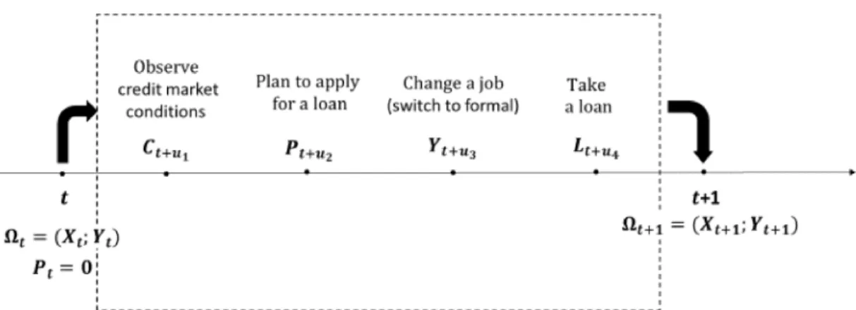
1.4.1 The Timeline of the Model
In the empirical model at the beginning of period t, the individual i can be in one of four
employment states j, Yijt: paid-employment (j = 0), Type-1 self-employment (j = 1), Type-2 self-employment (j = 2) or non-employment (j = 3). The individual i also has a set of time-varying individual characteristics Xit (e.g., age, years of schooling, marital status, the value of
large, durable assets and etc.) and constant individual characteristics Xt (e.g., gender, race and
Hispanic ethnicity). The agent observes the local CMA (the proximity of bank services) in period
t, Zit, that is a set of the following variables12: the average distance from the individual to 10
nearest banks, the number of banks and branches within 5 miles from the individual’s home, and
the number of bank workers per 1,000 population at the county level. The proximity of bank
services may create incentives for the individual i to change the labor state. For example, if the
use of bank services becomes cheaper for the self-employed, a person may make a decision to
become self-employed and open a new business; or if self-employed individualidoes not satisfy
bank requirements (e.g., annual income requirements, collateral requirements, credit score, etc.),
the person may make a decision to switch to paid employment to be able to use bank services. At
the beginning of periodt+ 1, one would observe a new employment state for individuali. 1.4.2 Dynamic Multinomial Logit Model of Employment
The purpose of this empirical analysis is to show how the proximity of bank services,Zit, with
explanatory variables, Xit and Xi, influences the transition between employment states Yijt →
Yijt+1, and I model this transition using the dynamic multinomial logit process with state
depen-dence and unobserved heterogeneity (Prowse 2012).
The probability of employment choicejcan be expressed as follows:
P rt+1(j|Xit, Zit, µij) =
exp(Yijtβ1j +Zitβ2j+Xitβ3j +µij) P
j0∈{P E,SE1,SE2,N E}exp(Yij0tβ1j0 +Zitβ2j0 +Xitβ3j0 +µij0)
(1.1)
The probability of employment choice j depends on the previous period job type, Yijt, and the
coefficient β1j shows the mobility of individuals across employment states between t and t+ 1. The error term, µij, represents time-variant unobservables. As a proxy for non-interest costs of
borrowing (or the distance measure between), I use the measure of the CMA,Zit. A higher value
of the CMA implies closer proximity to banking services. Since banks perform many functions, I
assume that future unobserved shocks do not influence the availability of banking services and an
individuals job choice in a given year. The measure of the CMA,Zit, is assumed to be exogenous
conditional on the time-constant unobserved effect (µij) time-varying observed factors that may
influence the opening of new bank offices in a given area, but I discuss later some potential
solu-tions to possible violasolu-tions of this assumption. β2j is another coefficient of interest that shows the
direct effect of the CMA on the type of employment. The agent’s ability,θ, the amount of available
assets,at+1, and the wage of a paid employed worker,wt+1are included inXit, and I will discuss
actual measures for these variables later.
The model can be re-written in a more conventional log-odds form by choosing the
non-employed type as the base category:
lnP r(Yit+1 =m, m∈ {P E, SE1, SE2}) P r(Yit+1 =N E)
=Yijtβ1j +Zitβ2j +Xitβ3j +µij (1.2)
1.4.3 Identification
Several issues arise in the estimation of equation 1.2. The first one is the possible correlation
of the unobserved heterogeneity,µij, with explanatory variables. Following the literature of
Mur-tazashvili and Wooldridge (2016), Papke and Wooldridge (2008), I add the Mundlak-Chamberlain
device or the longitudinal average of time-varying explanatory variables, Xit, which models the
permanent unobserved heterogeneity as a linear projection of the time average of time-varying
characteristics. This approach accounts for the endogeneity of inputs with regards to unobserved
factors like an individual fixed-effect model. Since the panel dataset used here is unbalanced, it is
impossible to apply the original approach suggested by Wooldridge (2005) and include a complete
history of lagged explanatory variables, Xt+ = (Xi2, ..., XiT)andZt+ = (Zi2, ..., ZiT). But I can apply the modified version of Wooldridge (2005) proposed by Rabe-Hesketh and Skrondal (2013),
who suggest using the within-means of individual time-varying characteristics based on all periods
excluding the first period observations, Xi+ = T1−1PT
t=2Xit and Z +
i =
1 T−1
PT
t=2Zit. X +
i and
Zi+ are an analog to the Mundlak-Chamberlain device but without initial values. This approach
accounts for the possible endogeneity of the CMA with regards to unobserved factors in a manner
similar to the fixed-effect model.
The second issue is related to the initial conditions and occurs due to the correlation betweenµij
and the initial observationYij1, and the endogenous initial conditions require a specification of the
conditional distribution forYij1.I address this problem using the solution suggested by Wooldridge
(2005) and Rabe-Hesketh and Skrondal (2013). This solution specifies the conditional distribution
of µij via an auxiliary model that includes an initial dependent variable, Yij1, the initial-period
explanatory variables, Xi1 and Zi1, and within-means of individual time-varying characteristics
based on all periods excluding the first period observations,Xi+. The model specifies the following
conditional density of the unobserved heterogeneity:
whereXi+ is the within-means of individual time-varying characteristics based on all periods
ex-cluding the first period observations Xi+ = T1−1PT
t=2Xit; Yij1 is the initial-period dependent variable; Xi1 is the initial-period explanatory variables; Zi+ is the withmeans of the CMA
in-dex based on all periods excluding the first period observations Zi+ = T1−1PT
t=2Zit; Zi1 is the initial-period CMA; ηij is the error term where Cov(ηij;υijt+1) = 0. The vector Gi consists of the initial dependent variable, initial explanatory variables, and within-means of explanatory
vari-ables in subsequent periods. The approach suggested by Wooldridge (2005) and Rabe-Hesketh
and Skrondal (2013) has several advantages. It does not require instruments, because the initial
conditions are not modeled separately (in contrast to Heckman (1987) approach). It can be applied
to unbalanced panels, and the within-means termsXi+ andZi+allow for the correlations between
the explanatory variables and the unobserved heterogeneity,µij.
The substitution of equation (1.3) into (1.2) leads to the standard random-effects multinomial
logit model:
lnP r(Yit+1 =m, m∈ {P E, SE1, SE2)}) P r(Yit+1 =N E)
=Yijtβ1j +Zitβ2j +Xitβ3j+Giπj+ηij (1.4)
To estimate the model with the unobserved heterogeneity, ηij, I use two approaches. In the
first approach, I assume multivariate normality of the error term, ηij ∼ N(0;ση2). In the second approach, I use a variation of the discrete factor approximation (Heckman and Singer 1984).
Endogenous Locations of Branches. Identification of the causal effect of the CMA on self-employment is challenging because the choice of where to locate a bank is not exogenous. In
particular, the decision to open or close a branch is endogenous to the local economic conditions
that also affect an individual’s home location and the decision to become self-employed. There
are several solutions to this issue. One possible solution is to control for a large set of variables
that proxy the local economic conditions at the county level, for example, the number of business
establishments, the unemployment rate, the share of the population with professional, scientific,
management and administrative education. For this approach, I add the above set of variables that
possible correlation of the unobserved individual permanent heterogeneity with the variables of
the local economic conditions and the initial condition problem, I include analogs to the
Mundlak-Chamberlain device,L+i = 1 T−1
PT
t=2Lit, and the initial period local economic conditions,Li1.
lnP r(Yit+1 =m, m∈ {P E, SE1, SE2)}) P r(Yit+1 =N E)
=Yijtβ1j +Zitβ2j +Xitβ3j +Litβ4j +Fiπj+ηij (1.5)
whereFiπj =π1jYij1+Xi+π2j+π3jXi1+Zi+π4j+π5jZi1+L+i π6j+π7jLi1.
Equation (1.5) is the main specification for the empirical part of the paper. I estimate equation
(1.5) using both of the estimation approaches to the unobserved heterogeneity,ηij, that I described
above.
Then, I estimate equation (1.5) using the lagged measure of the CMA, Zit−1. The one-year
measure of the CMA, Zit−1 is assumed to be exogenous conditional on the time-constant
unob-served effect (µij) and time-varying observed factors that may influence the opening of new bank
offices in a given area.
Another approach is to estimate model equation (1.5) only for individuals who remained at the
same location so any change in the borrower-lender distance was attributable to changes in banks’
location.
Finally, I used an instrumental variable for changes in the local CMA. I apply the
instru-ment suggested by Nguyen (2019) and Garmaise and Moskowitz (2006), which is the exposure to
merger-induced consolidation at the Census tract-level13.I consider mergers of large banks, defined
as mergers where both banks held at least US$1 billion in pre-merger assets. The average Census
tract is 1.5 square miles, and the decision of large banks to merge is plausibly exogenous to the
local economic conditions in a Census tract where both banks have a branch. The merge-induced
consolidation decreases competition between banks at the tract level, which may be followed by
a branch closure (Nguyen 2019), an increase in the borrower-lender distance, a decrease in the
number of branch employees and a decline in the local CMA.
The empirical framework for the instrumental variable approach is the dynamic multinomial
logit model with the CMA measure,Zit, treated as endogenous:
lnP r(Yit+1=m, m∈{P E,SE1,SE2)})
P r(Yit+1=N E) =Yijtβ1j +Zitβ2j +Xitβ3j+Litβ4j+Fiπj +ηiβ5j
Zit=Eitγ1+Yijtγ2+Xitγ3+Litγ4+Git+ηi
(1.6)
whereEit equals 1 if individualilives in a Census tract where two large banks merged in yeart,
Fiπj =π1jYij1+Xi+π2j+π3jXi1+Zi+π4j+π5jZi1+L+i π6j+π7jLi1,Git =Yij1ψ1+Xi+ψ2+
Xi1ψ3+Zi1ψ4+Li1ψ5+L+i ψ6. For computational simplicity, I assume thatηi ∈N(0; 1). Equation (1.6) jointly estimates the labor decisions of individualidue to changes in the CMA,
Zit, and the CMA as a function of the individual characteristics,Xit, the current labor state,Yijt,
the local economic conditions,Lit, and the instrumental variableEit. The error term,ηi, contains
the permanent individual unobserved heterogeneity that influences both the labor decisions and the
CMA for individuali.
1.5 Data
1.5.1 Sources of Data
This paper combines several sources of U.S. data. The primary source is the Community
Advantage Panel Survey (CAPS) database collected by the UNC Center for Community Capital.
CAPS comprises 11 years of panel survey data provided by approximately 5,000 low- and
moder-ate income homeowners and renters during the period of 2003-2014. The homeowners recruited
to participate in CAPS received mortgages between 1999 and 2003 through the Community
Ad-vantage Program, and the participating renters were recruited to match these homeowners with
respect to the geographic proximity and income ceilings. The survey collects a wide variety of
unemployment, wealth and asset holdings, social capital and civic engagement, and housing
sat-isfaction. The CAPS database was used in several works (e.g., Quercia, Freeman, and Ratcliffe
(2011), Manturuk, Lindblad, and Quercia (2017))14. The data Appendix provides more
informa-tion about the survey design.
Data on career choices and self-employment. CAPS contains self-reported information about the primary work activity at the time of the survey. The survey has four types of employment:
workers in private businesses, government workers, self-employed workers, and workers in a
family business. The first two categories workers in private businesses and government workers
-were combined as paid employed workers. Self-employed and workers in a family business are
different labor types due to various liabilities; therefore, I consider only self-employed in the
anal-ysis and exclude workers in a family business from the data sample.
Data on bank locations. All information about bank offices comes from the FDIC SOD data for 2003-2014 as of June 30 of the corresponding year. The SOD data include full street addresses
of bank headquarters and bank branches, the total amount of assets, and the latitude and longitude
of the bank headquarters and each bank branch since 2008. The maps in Figure 1.5 show the
location of all banks and branches from the FDIC SOD database (red dots) in 2003 and 2014. The
FDIC SOD contains information about 87,279 bank locations in 2003 and 94,521 bank locations
in 2014. Thus, the number of bank offices increased, but the locations are more concentrated. To
show the difference in concentration between 2003 and 2014, Figure 1.5 also reflects the hot spot
analysis (blue areas). The hot spot analysis shows the z-score for the Getis-Ord Gi* statistic for
each location in a dataset. Darker areas tell where bank locations with high values cluster spatially.
Bank addresses were transferred to geocodes15 and linked to home locations of CAPS
respon-dents in such a way that each respondent was linked to each bank within the same state. Bank
14The full list of publications is available at:https://communitycapital.unc.edu/files/2017/10/ Paper_22929_extendedabstract_1348_0.pdf
locations are used to identify the distance16from the location of a respondents home to banks (the
minimum distance; the distance to 5, 10, or 15 nearest banks); the number of banks per state, the
number of banks within 5, 10 or 15 miles from the respondent.
Other sources of data. Other sources of data include the U.S. Census Bureau Statistics (County Business Patterns), the Bureau of Labor Statistics Local Area Unemployment data
(county-level unemployment rates and civilian labor force size), the FDIC Assets and Liabilities report
(total number of employees per branch (full-time equivalent)), ACS county-level demographic
in-formation, and the Mergers and Acquisitions Database of the Federal Reserve Bank of Chicago17.
1.5.2 Explanatory Variables
As explanatory variables, I use a set of time-invariant individual characteristics, such as gender
(=1 if female), race (white, black, other), and Hispanic ethnicity. In addition, there are time-varying
variables, including the age, age squared, years of schooling, the spouse’s years of schooling, the
marital status, the household size, the number of children under the age of 14 currently living in the
household, the region, calendar year effects, the log of the value of large durable assets (houses,
land, other real estate and cars), the difference in log-income for wage and salary workers and
self-employed (non-incorporated) at the county level. The latter variable serves as a substitute
for individual income, which is likely to be endogenous. Unfortunately, CAPS does not contain
detailed information about wages or personal income, only aggregated household income.
As a measure of the local economic conditions, I use the total population at the zip-code level,
the share of the population with professional, scientific, management, and administrative education
at the zip-code level, the unemployment rate and the number of business establishments at the
county level.
16For estimating the distance, I use the SAS geocode procedure, because SAS allows to estimate distances without sending sensitive information to external servers, but the downside of using SAS is that it estimates the Euclidean distance between 2 locations. Boscoe, Henry, and Zdeb (2012) conclude that for nonemergency travel the added precision offered by the substitution of travel distance, travel time, or both for straight-line (Euclidean) distance is largely inconsequential.
1.5.3 Constructed Variables
Types of self-employment. The biggest challenge is how to identify different types of self-employment for the empirical analysis. Unfortunately, using the CAPS database, its impossible
to identify self-employed businesses without business loans (or with restricted access to the credit
market). In the empirical model, the main specification is based on types of self-employed
busi-nesses incorporated or unincorporated. Bopaiah (1998) shows that the incorporated self-employed
are more likely to get a business loan in comparison to the unincorporated self-employed, and
their businesses are more capital intensive. Levine and Rubinstein (2017) prove that incorporated
and unincorporated self-employed businesses demand different skills and abilities: the
incorpo-rated self-employed have comparatively strong nonroutine cognitive abilities, while the
unincor-porated self-employed are involved in businesses demanding relatively strong manual skills. Later,
Levine and Rubinstein (2018) differentiate between entrepreneurs and other self-employed and,
for empirical analysis, they use the incorporated self-employed as a proxy for the entrepreneurial
self-employed, and the unincorporated self-employed for other self-employed persons. For the
main specification, I adopt the approach proposed by Levine and Rubinstein (2018) and use the
incorporated employed as a proxy for the Type-1 employed, and the unincorporated
self-employed as a proxy for the Type-2 self-self-employed.
An alternative definition for different types of self-employment rests on the idea that
en-trepreneurial businesses are more capital intensive and more likely to depend on external funding.
A definition for types of self-employment can be also based on the degree to which a business
de-mands entrepreneurial abilities. Unfortunately, the database offers no assessment of respondents’
abilities. To evaluate the level of entrepreneurial skills, I use an external database O*NET
On-Line18. The database contains a list of occupations along with the level of entrepreneurship. The
level of entrepreneurship has a range between 1 and 5, where level 1 is equivalent to little or no
enterprising activities; level 5 is equal to an extensive level of entrepreneurship. Self-employed
workers are referred to Type-1 if the level of entrepreneurial activities is equal to 4 or 5; all other
self-employed workers are Type-2.
Another alternative definition of types of self-employment is based on the aggregate level of the
following characteristics: problem-solving, creation of new ideas, and thinking. Using the
charac-teristics of occupations from the O*NET OnLine database, I aggregate them into a standardized
z-score index. A higher value of the index means a higher level of problem-solving, creation of
new ideas and thinking. Self-employed workers with z-scores above 0 are referred to the Type-1
self-employed, all others - to the Type-2 self-employed.
One more definition of types of self-employment originates from studies on labor informality
in developing countries. In these studies, it is common to refer to small-scale self-employment
as the informal labor sector. Studies from countries with a large informal sector find that new
bank openings create incentives for individuals working in the informal sector to switch to jobs
with verifiable income to be eligible for loans and, thus, transit to paid employment (Malkova,
Peter, and Svejnar 2018). The share of self-employed individuals with unverifiable income may
fall when the borrower-lender distance decreases. Thus, the effect of the CMA on the transition to
self-employment may differ across individuals. The literature has not explored labor informality
broadly in the U.S., because the biggest challenge is the availability of data, and most American
surveys do not contain questions about informal labor activity. The study by Bracha and Burke
(2016) finds that 37 percent of non-retired U.S. adults participated in some informal work in 2015.
Due to the lack of other data and methodology for the labor informality in the U.S., I use the
non-participation in the earned income tax credit (EITC) program, if an individual is eligible for this
program, as a proxy for potential tax evasion. The Type-1 self-employed are self-employed persons
who participated in the EITC, while the Type-2 self-employed are those who did not engage in the
EITC even if they were eligible for this program. Workers not eligible for the EITC are excluded
Table 1.1: Alternative Definitions of Types of Self-Employment
Type 1 Type 2
Based on survey questions
1. Type of business Incorporated Unincorporated
2. Proxy for tax evasion Participation in EITC Non-participation in EITC
by eligible individuals by eligible individuals
Based on ILO occupation codes (matched to National Center for O*NET dataset)
3. Level of entrepreneurial abilities High entrepreneurial abilities Low entrepreneurial abilities
4. Level of abilities: problem solving, Z-score index>0 Z-score index≤0 creation of new ideas and thinking
Credit market accessibility. The CMA is measured as an index based on a combination of
the following variables: the average distance from an individual to 10 nearest banks, the number
of banks and branches within five miles from the individual’s home, the number of bank workers
per 1,000 population at the county level. These variables were aggregated into a standardized
z-score index. The z-z-score index is scaled in such a way that a higher value means better access
to the formal credit market (e.g., shorter borrower-lender distance). And, for the convenience of
interpretation, I standardize the CMA index with a mean of zero and a standard deviation of one.
Instrumental variable. To estimate equation (1.6), I create an instrumental variable,Eit, that
equals one if individualilives in a Census tract where two large banks undergo a merger in yeart,
and zero otherwise. To create the instrument, I use data on merger activity from the Mergers and
Acquisitions Database (M&A) of the Federal Reserve Bank of Chicago. Each buyer or target bank
has an RSSD ID that allows for matching the M&A database to the FDIC SOD; thereby, I can
identify branches that can be exposed to merger-induced consolidation. I consider mergers of large
banks, where both banks held at least US$1 billion in pre-merger assets. For all branch addresses
in the FDIC SOD, I identify the Census tract number applying the SAS geocode procedure. Using
these data, I identify tracts where branches of two large banks may be exposed to merger-induced
1.6 Results
In this section, I discuss my empirical findings and the implications for how an increase in the
CMA affects self-employment19. First, I present the results from the estimation of the dynamic
multinomial logit model of employment with correlated random effects using both parametric and
non-parametric approaches. For the main specification as given in equation (1.5), self-employment
is defined on the basis of the legal structure; the Type-1 and Type-2 self-employed are owners of
incorporated and unincorporated businesses respectively. Second, I use the estimated coefficients
to determine the average marginal effects (AMEs) of the CMA on the size of four employment
sectors and the transition probabilities among the sectors. Partly as a robustness check, I then
present the results from other specifications of the model and finally determine how improvements
in banking services across geographical areas affect self-employment.
1.6.1 Access to Credit Products
In this subsection, I discuss how the borrower-lender distance influences the access to credit
products. Unfortunately, CAPS data do not contain information about business-related lending,
and in a perfect situation, the effect of the CMA on labor decisions should be estimated through
the access to credit products. Using the available data, I highlight two main groups of variables
characterizing the access to credit: the access to different credit products and indicators of a
reduc-tion in the credit access. The variables describing the access to various products are a set of dummy
variables: if the respondent applied for a new credit card in the last 12 months, if the respondent
applied for a car loan in the last 12 months, if the respondent opened a new charge card in the
last 12 months, if the respondent refinanced a mortgage in the last 12 months. The indicators of
a reduction in the credit access are a set of dummy variables: if the respondent’s application for
a new credit was rejected in the last 12 months, if the respondent’s available limit for credit cards
was reduced in the last 12 months, if the respondent was asked to pay off the remaining balance
for a loan in the last 12 months, if the respondent filed bankruptcy in the last 12 months.
To evaluate the effect of the CMA on the access to credit, I estimate a random-effects
pro-bit model for each of the variables characterizing the access to credit. To avoid the problem
of a possible correlation of the unobserved individual permanent heterogeneity with
explana-tory variables, I include analogs to the Mundlak-Chamberlain device, Xi+ = T−11PT
t=2Xit and
L+i = T−11PT t=2Lit.
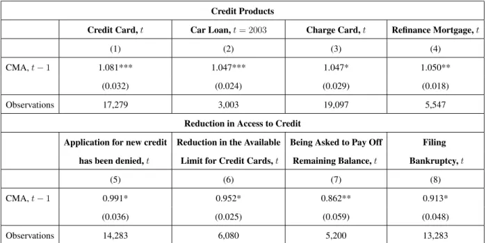
P r(Cit = 1) = Φ(Zit−1β1+Xitβ2+Litβ3+Xi+β4+L+i β5+νi) (1.7)
whereνi are i.i.d., νi ∈ N(0, σ2ν), andΦis the standard normal cumulative distribution function. Citis a dummy variable that equals 1 if the respondent applied for a new credit card in the last 12
months; if the respondent applied for a car loan in the last 12 months; if the respondent opened
a new charge card in the last 12 months; if the respondent refinanced a mortgage in the last 12
months; if the respondent’s application for a new credit was rejected in the last 12 months; if the
respondent’s available limit for credit cards was reduced in the last 12 months; if the respondent
was asked to pay off the remaining balance for a loan in the last 12 months; if the respondent filed
bankruptcy in the last 12 months.
The results of equation (1.7) are shown in Table 1.4. They suggest that an improvement in the
CMA (shorter borrower-lender distance) increases the probability of receiving a new credit card,
having a car loan, obtaining a charge card or refinancing a mortgage. These results support the
evidence from the literature that a shorter borrower-lender distance makes loans more affordable.
Another part of the results suggests that improvements in the CMA decrease the risk of a reduction
in the access to credit. A shorter borrower-lender distance reduces the risk of the application for a
new credit being rejected, a reduction in the available limit for credit cards, being asked to pay off
the remaining balance, and filing bankruptcy.
1.6.2 Results of the Main Model
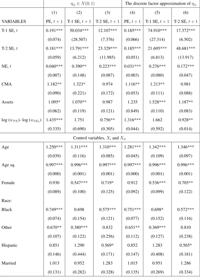
The results of the main model are reported in Table 1.5. The table presents the relative risk
ratios from the dynamic multinomial logit model of employment with correlated random effects.
as the base outcome and the paid employment state selected as the omitted lagged dependent
category. The table presents the results of the model for the main specification, and the type of
self-employment is defined based on the legal status of businesses the Type-1 self-employed are owners
of incorporated businesses, and the Type-2 self-employed are owners of unincorporated businesses.
Table 1.5 shows both of the estimation approaches for permanent unobserved heterogeneity. In this
subsection, I discuss the results for the parametric estimation,µij ∈ N(0, σν2); the results for the discrete factor approximation are very similar.
The previous labor status plays an essential role in the type of the current job. Predictably, for
self-employed and non-employed individuals, the risk of working in the paid employment sector in
periodt+ 1relative to paid employed workers is small and negative (the odds are 0.191, 0.181, and 0.040, respectively). For both types of the self-employed, the previous job in the self-employed
sector increases the risk of being either type of the self-employed. The relative risk ratio of being
Type-1 self-employed in periodt+ 1relative to paid employed workers in periodtis 50.034 for the Type-1 self-employed and 13.791 for the Type-2 self-employed. The non-employed are less likely
to switch to any type of self-employment. The relative risk ratio of being Type-2 self-employed in
periodt+ 1relative to paid employed workers in periodtfor the Type-1 self-employed and 23.329 for the Type-2 self-employed.
The result of primary interest is the coefficient of the CMA index. A one-standard-deviation
increase in the CMA index increases the odds of being paid employed by 1.182. At the same time,
a one-standard-deviation improvement in the CMA increases the relative risk of becoming Type-1
self-employed by 1.323. But the relative risk ratio for the Type-2 self-employed is insignificant.
The value of large, durable assets plays an essential role in being self-employed and increases
the risk of being Type-1 self-employed or Type-2 self-employed, but it does not significantly
in-fluence the risk of being a paid employed worker. Furthermore, the difference in log-income for
wage and salary workers and self-employed workers increases the risk of being paid employed,
decreases the risk of being Type-2 self-employed, and does not influence the risk of being Type-1
self-employed.
transition probabilities, I re-estimate the main model including the interaction terms between the
employment state,Yijt, and the credit market accessibility index,Zit:
lnP r(Yit+1 =m, m∈ {P E, SE1, SE2)}) P r(Yit+1=N E)
=Yijtβ1j+Zitβ2j +Yijt∗Zitβ3j+Xitβ4j+
+Litβ5j+Fiπj +ηij
(1.8)
whereFiπj =π1jYij1+Xi+π2j+π3jXi1+Zi+π4j+π5jZi1+L+i π6j+π7jLi1.
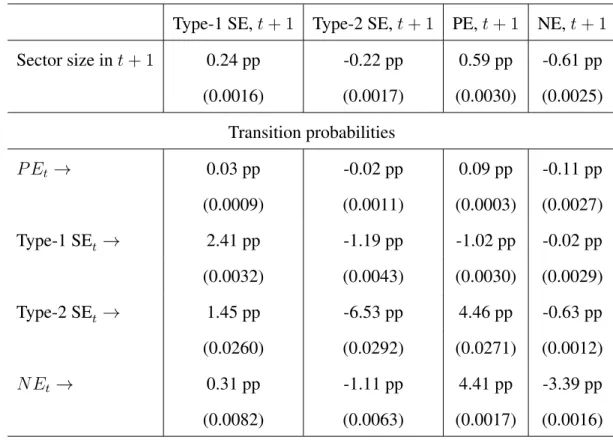
Table 1.6 presents the AME of a one-unit improvement in the CMA index on the size of
sec-tors. This one-unit improvement in the CMA index increases the population share of the Type-1
self-employed by 0.24 ppt and reduces that of the Type-2 self-employed by 0.22 ppt. Table 1.6
also shows the average marginal effect (AME) ofZit on the probability of switching between
em-ployment states. For the Type-1 self-employed, an increase inZit by one standard deviation raises
the likelihood of turning from paid-employment to self-employment by 0.03 ppt. The effect ofZit
on the likelihood of staying in the Type-1 self-employment sector is substantial (2.41 ppt
improve-ment). Similarly, there is a substantial positive effect on the probability of moving from the Type-2
self-employed (1.45 ppt). For non-employed individuals, the effect is 0.31 ppt. For Type-2
occupa-tions, the effect is the opposite. An improvement in the CMA (by one standard deviation) decreases
the chances of paid-employed workers to become Type-2 self-employed by 0.02 ppt. The effect
for the Type-1 self-employed is -1.19 ppt. The likelihood of staying in the self-employed sector for
Type-2 occupations goes down by 6.53 ppt per unit increase inZit. The AMEs for non-employed
individuals are smaller in magnitude, but they are still substantial. The transition probability from
the non-employed status to the Type-2 self-employed goes down by 1.11 ppt. The probabilities of
transition to paid employment are important results. A one standard deviation improvement in the
CMA decreases the probability of switching from Type-1 self-employment to paid employment by
1.02 percentage points. But for Type-2 self-employment, an improvement in the CMA increases
the probability of switching to paid employment by 4.46 ppt, which supports the evidence from
the theoretical model (Corollary 1) that a reduction of non-interest costs of borrowing is likely to
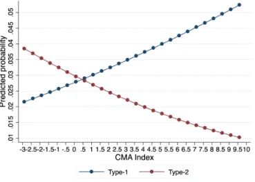
In addition to the AMEs (which are calculated across all individuals in the sample), I also
estimate the marginal effects at the mean values of covariates and at different values of Zit. These
results are plotted in Figure 1.8. The figure shows the predicted probabilities of being Type-1 or
Type-2 self-employed at different values of the CMA index. The results show a rise in the size of
the Type-1 self-employed and a decline in the Type-2 self-employed as the CMA improves.
1.6.3 Robustness Analysis
In this section, I discuss the results of several robustness analyses. First, I compare the
re-sults of the main model (equation1.5) for different distributional assumptions for the unobserved
heterogeneity. I estimate the main model (equation 1.5) under assumptions about the multivariate
normality of the error term and the discrete factor approximation of the error term. As I mentioned
in the previous section, rthe results for both distributional assumptions produce similar effects
(Ta-ble 1.5). Second, I compare the results of the main model (equation 1.5) for different definitions of
self-employed types (Table 1.7). Third, I show the results for different identification assumptions
for possible endogeneity of the CMA, that I described in the Identification section (Table 1.8).
Last, I show the results of the main model (equation 1.5) for the definition of self-employed types
based on potential tax evasion (last three columns in Table 1.7) and draw comparisons with the
literature on developing countries.
Different definitions of self-employed types. The results of the main model (equation1.5)
al-ternative definitions of self-employed groups are presented in Table 1.7. Columns (1)-(3) show the
results of the main specification discussed above. Columns (4)-(6) present the results of the model
when the definition of types of the self-employed is based on the degree to which the business
demands entrepreneurial abilities. Columns (7)-(9) present the results of the model when the
defi-nition of types of the self-employed is based on aggregate characteristics of occupations. Columns
(10)-(12) present the results of the model when the definition of types of the self-employed is
based on participation in the EITC program (I discuss these results later). In all specifications, a
one-standard-deviation improvement in the CMA increases the relative risk of becoming Type-1
self-employed and paid employed.
identification assumptions discussed in the ”Identification” section. The result of primary interest
is the coefficient of the CMA index. For the base specification under an assumption about the
exogenous CMA, a one-standard-deviation increase in the CMA index increases the odds of being
paid employed by 1.103. At the same time, a one-standard-deviation improvement in the CMA
increases the relative risk of becoming Type-1 self-employed by 1.197. But the relative risk ratio
for the Type-2 self-employed is insignificant. The results for other identification assumptions are
similar: including a lag for the CMA, estimating the model only for individuals who did not move
from their original place of living, and including the local economic condition (within-means of the
local economic condition and the initial conditions). It is interesting that the results for the latter
specification, including the Mundlak-Chamberlain device for the CMA and the initial value of the
CMA, show even higher relative risk ratios. A one-standard-deviation increase in the CMA index
increases the odds of being paid employed by 1.207, and a one-standard-deviation improvement in
the CMA increases the relative risk of becoming Type-1 self-employed by 1.376.
The results for equation (1.6), which jointly estimates the labor decisions of individual idue
to changes in the CMA, and the CMA as a function of the local economic conditions and the
instrumental variable, are shown in Table 1.9. The instrumental variable equals one if individual
i lives in a Census tract where two large banks undergo a merger in year t. The results show that
the exposure to merger-induced consolidation negatively influences the CMA. A
one-standard-deviation increase in the CMA index increases the odds of being paid employed by 1.097. At
the same time, a one-standard-deviation improvement in the CMA increases the relative risk of
becoming Type-1 self-employed by 1.188. But, the relative risk ratio for the Type-2 self-employed
is insignificant.
Tax evasion and labor informality. The last three columns of Table 1.7 provide the results for estimation of the main model (equation 1.5) with the definition of types of the self-employed
based on participation in the EITC program. I use non-participation in the EITC program if the
individual is eligible for this program as a proxy for potential tax evasion20. The results show
that a one-standard-deviation improvement in the CMA increases the relative risk of becoming
Type-1 self-employed and paid employed but decreases the risk of being Type-2 self-employed.
These results support the evidence from studies about labor informality in developing countries
(Malkova et al., 2019). Unfortunately, the literature has not explored labor informality broadly
in the U.S. Bracha and Burke (2016) find that 37 percent of non-retired U.S. adults participated
in some type of informal work in 2015. The biggest challenge is the data availability because
primary American surveys dont contain questions about informal labor activity. Bracha, Burke,
and Khachiyan (2015)21mention that the Survey of Informal Work Participation within the Survey
of Consumer Expectations (SCE-SIWP) is the only one that covers a nationally representative
sample.
1.7 Conclusion
The paper investigates the role of the credit market channel in the decrease of self-employment
in the U.S. To analyze the impact of the CMA on entry into self-employment, I develop a
three-sector Roy model that differentiates between two types of the self-employed: entrepreneurs who
have growth-oriented businesses that demand physical capital and business loans (Type-1) and
other self-employed (Type-2). The focus of the study is the physical accessibility of banks, and
I use a novel data source (the Community Advantage Panel Survey database) that allows me to
measure the proximity of credit market institutions for all respondents in the dataset. A
combi-nation of the following variables creates the index of physical availability of banks: the average
distance from the respondent’s home to 10 nearest banks, the number of banks within 5 miles from
the location of the respondent’s home, and the average number of workers per bank’s office at the
county level.
The empirical study estimates how the selection into self-employment can be driven by credit
market institutions using the dynamic multinomial logit model of employment with correlated
random effects. The analysis shows a heterogeneous response to changes in the CMA among