Introduction to GNU Octave
A brief tutorial for linear algebra and calculus students
A brief tutorial for linear algebra and calculus students
Jason Lachniet
Wytheville Community College
©2020 by Jason Lachniet (CC-BY-SA)
This work is licensed under a Creative Commons Attribution-ShareAlike 4.0 International Li-cense. To view a copy of this license, visithttp://creativecommons.org/licenses/by-sa/4. 0/or send a letter to Creative Commons, PO Box 1866, Mountain View, CA 94042, USA. Edition 3
Download for free at:
Contents
Contents vii
Preface ix
1 Getting started 1
1.1 Introduction . . . 1
1.2 Navigating the GUI . . . 3
1.3 Matrices and vectors . . . 4
1.4 Plotting . . . 9
Chapter 1 Exercises . . . 14
2 Matrices and linear systems 17 2.1 Linear systems . . . 17
2.2 Polynomial curve fitting . . . 23
2.3 Matrix transformations . . . 27
Chapter 2 Exercises . . . 33
3 Single variable calculus 39 3.1 Limits, sequences, and series . . . 39
3.2 Numerical integration . . . 43
3.3 Parametric, polar, and implicit functions . . . 46
3.4 The symbolic package . . . 50
Chapter 3 Exercises . . . 57
4 Miscellaneous topics 59 4.1 Complex variables . . . 59
4.2 Special functions . . . 61
4.3 Statistics . . . 63
Chapter 4 Exercises . . . 70
5 Eigenvalue problems 73 5.1 Eigenvectors . . . 73
5.2 Markov chains . . . 74
5.3 Diagonalization . . . 78
5.4 Singular value decomposition . . . 82
5.5 Gram-Schmidt and the QR algorithm . . . 88
Chapter 5 Exercises . . . 93
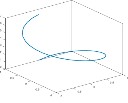
6 Multivariable calculus and differential equations 97 6.1 Space curves . . . 97
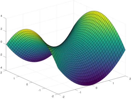
6.2 Surfaces . . . 99
6.3 Multiple integrals . . . 108
6.4 Vector fields . . . 114
6.5 Differential equations . . . 117
Chapter 6 Exercises . . . 124
7 Applied projects 127
7.1 Digital image compression . . . 127
7.2 The Gini index . . . 130
7.3 Designing a helical strake . . . 133
7.4 3D-printing . . . 136
7.5 Modeling a cave passage . . . 143
7.6 Modeling the spread of an infectious disease . . . 152
A MATLAB compatibility 157
B Octave command glossary 159
References 163
Preface
This short book is not intended to be a comprehensive manual (for that refer to [3], which is indispensable). Instead, what follows is a tutorial that puts Octave to work solving a selection of applied problems in linear algebra and calculus. The goal is to learn enough of the basics to begin solving problems with minimum frustration. Note that minimum frustration does not meannofrustration. Be patient!
Above all, our objective is simply to enhance our understanding of calculus and linear algebra by using Octave as a tool for computations. As we work through the mathematical concepts, we will learn the basics of programming in Octave. Note that while we deal with plenty of useful numerical algorithms, we do not address issues of accuracy and round-off error in machine arithmetic. For more details about numerical issues, refer to [1].
How to use this book
To get the most out of this book, you should read it alongside an open Octave window where you can follow along with the computations (you will want paper and pencil, too, as well as your math books). To get started, read Chapter1, without worrying too much about any of the mathematics you don’t yet understand. After grasping the basics, you should be able to move into any of the later chapters or sections that interest you.
Every chapter concludes with a set of problems, some of which are routine practice, and some of which are more involved. Chapter 7 contains a series of applied projects. Most examples assume the reader is familiar with the mathematics involved. In a few cases, more detailed explanation of relevant theorems is given by way of motivation, but there are no proofs. Refer to the linear algebra and calculus books listed in the references for background on the underlying mathematics. In the spirit of openness, all references listed are available for free under GNU or Creative Commons licenses and can be accessed using the links provided.
MATLAB
The majority of the code shown in this book will work inMatlabas well as Octave. This guide
can therefore also be used an introduction to that software package. Refer to Appendix A for some notes onMatlabcompatibility.
Formatting
Blocks of Octave commands are indented and displayed with special formatting as follows.
>> % example Octave commands :
>> x = [−3 : 0 . 1 : 3 ] ;
>> p l o t( x , x . ˆ 2 ) ;
>> t i t l e('Example p l o t')
The same formatting is used for commands that appear inline in the text. Comments used to explain the code are preceded by a%-sign and shown ingreen. Function names are highlighted inmagenta. Strings (text variables) are highlighted inpurple. The Octave prompt is shown as “>>”. This color coding visible in thepdfe-book is not essential to understand the text. Thus
the print version is in black and white, which keeps the price reasonable.
Octave scripts and function files (.m-files) are shown between horizontal rules and are labeled with a title, as in the following example. These are short programs in the Octave language.
Octave Script 1: Example
1 % T h i s i s an example Octave s c r i p t ( . m−f i l e ) 2 t = l i n s p a c e( 0 , 2*p i, 5 0 ) ;
3 x = c o s( t ) ; 4 y = s i n( t ) ; 5
6 % p l o t t h e graph o f a u n i t c i r c l e 7 p l o t( x , y ) ;
Note that line numbers are for reference purposes only and are not part of the code
If you are reading the electronicpdfversion, there are numerous hyperlinks throughout the text
that link back to other parts of the text, or to external urls. There is a set of bookmarks to each chapter and section that can be used to easily navigate from section to section. Open the bookmark link in yourpdf viewer to use this feature.
Theorems and example problems are numbered sequentially by chapter and section (e.g., The-orem 5.3.4 is the fourth numbered item in Chapter 5, Section 3).
Solutions to the many example problems are offset with a bar along the left side of the page, as shown here. A box signifies the end of the example.
Feedback
If you use the book and find it helpful, please consider leaving a review on the Amazon.com
Revision history
2017 First edition
• Written for Octave version 4.0.
2019 Second edition
• Updated to reflect changes implemented in Octave through version 4.4, includ-ing the addition of a variable editor, migration of some statistical functions to the statistics package, and the addition of Matlab-compatible ODE solvers to the Octave core.
• New material added on implicit plots, complex variables, matrix transforma-tions, and symbolic operations.
• Addition of several new exercises and a new chapter containing a set of applied projects suitable for linear algebra and calculus students.
2020 Third edition
• Updated for Octave version 5.2.
• More extensive three-dimensional plotting examples. • Increased coverage of the symbolic package.
• Numerous small edits throughout to improve clarity of exposition, based on reviewer and student feedback.
• Multiple new or revised exercises throughout, and one new project.
Getting started
1.1
Introduction
1.1.1 What is GNU Octave?
GNU Octave is free software designed for scientific computing. It is intended primarily for solving numerical problems. In linear algebra, we will use Octave’s capabilities to solve systems of linear equations and to work with matrices and vectors. Octave can also generate sophisticated plots. For example, we will use it in vector calculus to plot vector fields, space curves, and three dimensional surfaces. Octave is mostly compatible with the popular “industry standard” commercial software package Matlab, so the skills you learn here can be applied to Matlab
programming as well. In fact, while this guide is meant to be an introduction to Octave, it can serve equally well as a basic introduction toMatlab.
What is “GNU?” Agnuis a type of antelope, but GNUis a free, Unix-like computer operating system. GNU is a recursive acronym that stands for “GNU’s not Unix.” GNU Octave (and many other free programs) are licensed under the GNU General Public License: http://www. gnu.org/licenses/gpl.html.
Fromwww.gnu.org/software/octave:
GNU Octave is a high-level interpreted language, primarily intended for numerical computations. It provides capabilities for the numerical solution of linear and non-linear problems, and for performing other numerical experiments. It also provides extensive graphics capabilities for data visualization and manipulation. Octave is normally used through its interactive command line interface, but it can also be used to write non-interactive programs. The Octave language is quite similar to
Matlabso that most programs are easily portable.
Octave is a fully functioning programming language, but it is not a general purpose programming language (like C++, Java, or Python). Octave is numeric, not symbolic; it is not a computer
Figure 1.1: Windows Octave GUI
algebra system (like Maple, Mathematica, or Sage)1. However, Octave is ideally suited to all types of numeric calculations and simulations. Matrices are the basic variable type and the software is optimized for vectorized operations.
1.1.2 Installing Octave
It’s free! Octave will work with Windows, Macs, or Linux. Go to https://www.gnu.org/ software/octave/download.html and look for the download that matches your system. For example, Windows users can find an installer for the current Windows version at https: //ftp.gnu.org/gnu/octave/windows/. Manual installation can be tricky, so look for the most recent .exe installer file and run that. Installation in most Linux systems is easy. For exam-ple, in Debian/Ubuntu, run the command sudo apt-get install octave. If you find Octave useful, consider making a donation to support the project athttps://www.gnu.org/software/ octave/donate.html.
Beginning with version 4.0, Octave uses a graphical user interface (GUI) by default. When you start Octave, you should see something like Figure 1.1.
The user can customize the arrangement of windows. By default, you will have a large command window, which is where commands are entered and run, a file browser, a workspace window displaying the variables in the current scope, a command history, and beginning with version 4.4, a variable editor.
1.2
Navigating the GUI
1.2.1 Command history
In Octave, you can save variables that you defined in your session, but this does not save the commands you used, or a whole worksheet. Octave does have a command history that persists between sessions, so past commands can be brought up using the up arrow key, or using the command history list in the GUI.
If you want to save a series of commands that can be reopened, edited, and run again, you can create an Octave script, also known as an .m-file. This will be described in more detail in Chapter3 (see Section3.2.2).
1.2.2 File browser
Within the Octave graphical user interface, you should see your current directory listed near the top left. You can click the folder button to navigate to a different directory, such as the desktop, a flash drive, or a folder dedicated to Octave projects. The default start-up directory (and many other options) can be modified in the Octave start-up file.octaverc, or theMatlab-compatible
equivalentstartup.m.
1.2.3 Workspace
Under the file menu, the option “save workspace as” will allow you to saveall variables in the current scope. The workspace panel lists the current variables. An individual variable can be saved from the variable editor, described below. You can use the “load workspace” option under the file menu to load previously saved variables. Alternately, a variable or workspace file can be loaded by double-clicking on its name in the file browser.
Another approach is to use the manual saveand load commands at the command line. If you typesave FILENAME var1 var2 ..., Octave will save the specified variables in the fileFILENAME. If you do not supply a list of variables, then all variables in the current scope will be saved. You can then reload the saved variable(s) at another time by navigating to the appropriate directory and usingload FILENAME.
1.2.4 The variable editor
The variable editor allows displaying or editing a variable in a simple spreadsheet format. To use it, double click on the name of the variable in the workspace panel. You can undock the variable editor and maximize it is as a standalone window to facilitate working with larger arrays. If you want to enter data in a variable that does not already exist, you will need to preallocate a matrix of the correct size, for example using the command A =zeros(m, n) to create anm×n
1.2.5 Getting help
The full Octave software manual is accessible by changing to the documentation tab at the bottom of the screen, or the shell commandhelpcan be used at the Octave prompt. In particular, if you know the name of the command you want to use,help NAME will give the correct syntax. A basic command glossary is available in Appendix B.
Besides the present volume, here are two good free resources to help you get started quickly:
Simple Examples (from the Octave Manual [3]):
https://octave.org/doc/v4.0.1/Simple-Examples.html Wikibooks Tutorial:
https://en.wikibooks.org/wiki/Octave_Programming_Tutorial
Additional help can be found with internet searches. Depending on what you are looking for, searches for Octave commands and searches forMatlabcommands can both be useful. Numer-ous commercial user’s guides and textbooks for Octave and/or Matlab are available. Linear
algebra textbooks sometimes containMatlabcode examples and these generally work in Octave
as well.
1.3
Matrices and vectors
1.3.1 Basic arithmetic
The best way to get started is to try some simple problems. Use the following examples as a tutorial to learn your way around the program. Octave knows basic arithmetic and uses the standard order of operations. Try some simple computations:
>> 6/2 + 3*( 7 − 4 ) ˆ2
ans = 30
Octave ignores white space, so 6/2 and 6 / 2 are interpreted the same way. You can’t take shortcuts and leave out implied operations, though. For example, 3(7 −4) will give an error. Use 3*(7−4).
Vectors and matrices are basic variable types, so it is easier to learn Octave syntax if you already know a little linear algebra. Try this example to enter a row vector and name itu. You do not need to enter the comments (indicated by the % sign).
>> u = [ 1 −4 6 ] % row v e c t o r
u = % v a r i a b l e name
1 −4 6 % o u t p u t
To create a column vector instead, use semicolons:
>> u = [ 1 ; −4; 6 ] % column v e c t o r
u = % v a r i a b l e name
1 % o u t p u t
−4 6
Notice that the function of the semicolon is to begin a new row. The same basic syntax is used to enter matrices. For example, here is how to define a 3×3 matrix:
>> A = [ 1 2 −3; 2 4 0 ; 1 1 1 ] % m a t r i x
A = % v a r i a b l e name
1 2 −3 % o u t p u t
2 4 0
1 1 1
In Octave, all of the above variables are really just matrices of different dimensions. A scalar is essentially a 1×1 matrix. Similarly, a row vector is a 1×n matrix and a column vector is an
m×1 matrix. In the following sections we will take a closer look at the nuances of vector and matrix operations.
1.3.2 Vector operations
We’ll start with some simple examples. First, re-enter the column vector u from above, if it is not already in memory.
>> u = [ 1 ; −4; 6 ]
Now enter another column vector v and try the following vector operations which illustrate linear combinations, dot product, cross product, and norm (length).
>> v = [ 2 ; 1 ; −1] v =
2 1
−1
>> 2*v + 3*u % l i n e a r c o m b i n a t i o n
ans =
7
−10 16
>> d o t( u , v ) % d o t p r o d u c t
ans = −8
ans =
−2 13 9
>> norm( u ) % l e n g t h o f v e c t o r u
ans = 7 . 2 8 0 1
Try a few more operations:
Find cross(v, u). How does that compare tou×v? Calculate the length ofv,||v||, using norm(v).
Normalize v by calculating v/||v||. This gives a unit vector that points in the same direction asv.
Now let’s try a more complicated vector geometry problem, to see some of Octave’s potential.
*
-θ
u
projv(u) v
Figure 1.2: Vector projection
Theprojection ofuonto v, denoted projv(u), is the component ofuthat points in the direction of v. This can be thought of as the shadow u casts onto v from a direction orthogonal to v, as shown in Figure 1.2. To find the magnitude of the projection, use basic right-triangle trigonometry:
kprojv(u)k=kukcos(θ) Then, sinceu·v=kukkvkcos(θ),
kprojv(u)k = kukcos(θ) = kuk u·v
kukkvk
= kuv·vk
This is known as the scalar projectionof u onto v. Thevector projection onto vis obtained by multiplying the scalar projection by a unit vector that points in the direction of v. Thus,
projv(u) = ukv·vkkvvk = kuv·kv2(v) Since v·v=kvk2, this can also be written as:
The operations needed for vector projection are easily carried out in Octave. As an example, we will find the projection ofu=h3,5i onto v=h7,2i.
>> u = [ 3 5 ] u =
3 5
>> v = [ 7 2 ] v =
7 2
>> d o t( u , v ) / (norm( v ) ) ˆ2*v
ans =
4 . 0 9 4 3 1 . 1 6 9 8
Thus projv(u) =h4.0943,1.1698i. Later, in Example 5.5.2, we will see how to create our own user-defined function to automate the above steps.
1.3.3 Matrix operations
Matrix operations are simple and intuitive in Octave. We’ll start with multiplication.
LetA=
1 2 −3 2 4 0 1 1 1
and B =
1 2 3 4 0 −2 −4 6 1 −1 0 0
. Find AB.
>> A = [ 1 2 −3; 2 4 0 ; 1 1 1 ] % m a t r i x
A = % v a r i a b l e name
1 2 −3 % o u t p u t
2 4 0
1 1 1
>> B = [ 1 2 3 4 ; 0 −2 −4 6 ; 1 −1 0 0 ] B =
1 2 3 4
0 −2 −4 6
1 −1 0 0
>> A*B % m u l t i p l y A and B
ans = % r e s u l t s t o r e d a s 'ans'
−2 1 −5 16 % answer
2 −4 −10 32
2 −1 −1 10
Arithmetic operations in Octave are always assumed to be matrix operations, unless otherwise specified (see Section 1.4.1). Therefore, for A and B defined as above, we can compute things like 4A orAB by entering, respectively, 4*A or A*B, but operations like B*A or A+B throw errors (why?).
To get the transpose of a matrix, use the single quote2. For example, try calculatingBTA. >> B' *A % B' i s t h e t r a n s p o s e o f B
ans =
2 3 −2
−3 −5 −7
−5 −10 −9
16 32 −12
To perform basic matrix arithmetic, we also need identity matrices, which are easy to generate with theeye(n) command, where n is the dimension of the matrix. Let’s find 2A−4I.
>> 2*A − 4*e y e( 3 ) % e y e ( 3 ) i s a 3 x3 i d e n t i t y m a t r i x
ans =
−2 4 −6
4 4 0
2 2 −2
Octave can also find determinants, inverses, and eigenvalues. For example, try these commands.
>> d e t(A) % d e t e r m i n a n t
ans = 6
>> i n v(A) % m a t r i x i n v e r s e
ans =
0 . 6 6 6 6 7 −0.83333 2 . 0 0 0 0 0 0 . 3 3 3 3 3 0 . 6 6 6 6 7 −1.00000 0 . 3 3 3 3 3 0 . 1 6 6 6 7 0 . 0 0 0 0 0
>> e i g(A) % e i g e n v a l u e s
ans =
4 . 5 2 5 1 0 + 0 . 0 0 0 0 0 i 0 . 7 3 7 4 5 + 0 . 8 8 4 3 7 i 0 . 7 3 7 4 5 − 0 . 8 8 4 3 7 i
Notice that our matrix has one real and two complex eigenvalues. Octave handles complex numbers, of course! Eigenvalues will be discussed in more detail in Chapter 5. Octave can also compute many other matrix values, such as rank:
>> rank(A) % m a t r i x rank
ans = 3
Figure 1.3: Default graph of y= sin(x) on [0,2π]
1.4
Plotting
Basic two-dimensional plotting of functions in Octave is accomplished by creating a vector for the independent variable and a second vector for the range of the function. There are several forms for the syntax and we will attempt to outline the simplest methods here3.
Let’s start by plotting the graph of the function sin(x) on the interval [0,2π] (Figure 1.3). Like a typical graphing calculator, Octave will simply plot a series of points and connect the dots to represent the curve. The process is less automated in Octave (but in the end, much more powerful). We begin by creating a vector ofx-values.
>> x = l i n s p a c e( 0 , 2*p i, 5 0 ) ;
Notice the formatlinspace( start val , end val, n). This creates a row vector of 50 evenly spaced values beginning at 0 and going up to 2π. The smaller the increment, the smoother the curve will look. In this case, 50 points should be suitable. The semicolon at the end of the line is to suppress the output to the screen, since we don’t need to see all the values in the vector. Now, we want to create a vector of the correspondingy-values. Use this command:
>> y = s i n( x ) ;
Now, to plot the function, use the plot command: >> p l o t( x , y ) ;
Figure 1.4: Improved graph of y= sin(x) on [0,2π]
You should see the graph off(x) = sin(x) pop up in a new window.
Figure 1.3 shows the default graph. You may wish to customize it a little bit. For example, the x-axis extends too far. We can set the window with the axis command. The window is controlled by a vector of the form [Xmin Xmax Ymin Ymax]. Let’s set the axes to match the domain and range of the function.
>> a x i s( [ 0 2*p i −1 1 ] ) ;
We may want to change the color (to, say, red) or make the line thicker. We can add a grid to help guide our eye. In addition, a graph should usually be labeled with a title, axis labels, and legend. Try these options to get the improved graph shown in Figure1.4.
>> p l o t( x , y , 'r', 'l i n e w i d t h', 3 )
>> g r i d on
>> x l a b e l('x') ;
>> y l a b e l('y') ;
>> t i t l e('S i n e graph') ;
>> l e g e n d('y=s i n ( x )') ;
Note that some adjustments, like zooming in, or turning on the grid, can be done within the graph window using the controls provided. Some standard color options are red, green, blue, cyan, and magenta, which can be specified with their first letter in single quotes.
Figure 1.5: Scatter plot with regression line
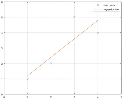
the workspace and clear any existing graphs. Then define a vector of x-values and a vector of
y-values and use the plot command. >> c l e a r; c l f ;
>> x = [ 1 2 3 4 ]
>> y = [ 1 2 5 4 ]
>> p l o t( x , y , 'o')
Now suppose we want to graph the liney= 1.2xon the same set of axes (this is the line of best fit for this data). To add to our current graph we need to use the commandhold on. Then any new plots will be drawn onto the current axes. We can switch back later withhold off .
>> h o l d on
>> p l o t( x , 1 . 2*x )
Now we should see four points and the graph of the line. Alternately, we can create multiple plots within a singleplot command. Try this, for example:
>> c l e a r; c l f ;
>> x = [ 1 2 3 4 ] ;
>> y1 = [ 1 2 5 4 ] ;
>> y2 = 1 . 2*x ;
>> p l o t( x , y1 , 'o', x , y2 )
>> a x i s( [ 0 5 0 6 ] ) ;
>> g r i d on ;
>> l e g e n d('d a t a p o i n t s', 'r e g r e s s i o n l i n e') ;
Figure 1.6: Graph ofy =x2sin(x)
1.4.1 Elementwise operations
An important consideration when working with a more complex function like, say,y=x2sin(x), is that Octave will regard the product and exponent as matrix operations, unless we indicate otherwise. The same is true for division. To avoid errors when we are evaluating a function at a numeric input vector, we need to use theelementwiseversions of exponentiation, multiplication, and division between variables. This is done by preceding the operation in question with a period, as in .ˆ or .* or ./.
These commands are incorrect and will cause errors:
>> x = l i n s p a c e(−10 , 1 0 , 1 0 0 ) ;
>> p l o t( x , x ˆ2*s i n( x ) ) % i n c o r r e c t s y n t a x : n o t e l e m e n t w i s e o p e r a t i o n s
e r r o r : f o r Aˆb , A must be a s q u a r e m a t r i x . Use . ˆ f o r e l e m e n t w i s e power . e r r o r : e v a l u a t i n g argument l i s t e l e m e n t number 2
But this will do the trick:
>> x = l i n s p a c e(−10 , 1 0 , 1 0 0 ) ;
>> p l o t( x , x . ˆ 2 .*s i n( x ) ) % c o r r e c t : e l e m e n t w i s e e x p o n e n t and p r o d u c t
The result is shown in Figure1.6.
1.4.2 Plot options
The following table summarizes some standard options that can be used with theplotcommand.
Plot options
marker '+' crosshair color 'k' black
'o' circle 'r' red
'*' star 'g' green
'.' point 'b' blue
's' square 'm' magenta
'ˆ' triangle 'c' cyan
size 'linewidth', n (n is some positive value)
'markersize', n
line style '−' solid line (default)
'−−' dashed line
':' dotted line
Several options may be combined. For example,plot(x, y, 'ro :') indicates red color with circle markers joined by dotted lines.
Here are several key functions for providing textual labels:
Plot labels
horizontal axis label . . . . xlabel('axis name'); vertical axis label . . . ylabel('axis name');
legend . . . legend('curve 1', 'curve 2', ...) ; title . . . title('plot title ') ;
The position of the legend may be modified using the commandlegend('location', 'position'), where “position” is a string giving a compass position, like northeast (which is the default), north, south, east, southwest, etc. Typehelp legend for a full list of options.
1.4.3 Saving plots
If we have created a good plot, we probably want to save it. The easiest option is to use copy and paste from the plot window. You can also use the “save as” option under the file menu to save the plot in various image formats.
An alternate method is to save the plot directly by “printing” it to a file. Octave supports several image formats. In the example below, thepngformat is used. To save the current graph
as apng, use this syntax:
>> p r i n t f i l e n a m e . png −dpng
Here filename.png is whatever file name you want (include the extension). You can replace
pngwith other image formats, such asjpgoreps. The file will be saved in your current working
Chapter
1
Exercises
Begin each problem with no variables stored. You can clear any previous results with the command clear.
1. For practice saving and loading variables, try the following.
(a) Create a new directory called “octave projects”.
(b) Change to the octave projects directory.
(c) Save the example matrices A and B from above in a text file namedmatrices.mat. (d) Quit Octave.
(e) Restart Octave and reload the saved matrices.
2. Letu=h2,−4,0i andv=h3,1.5,−7i. Find each of the following.
(a) w= 2u+ 5v
(b) d=u·v
(c) l=||u||
(d) u1 = a unit vector that points in the direction ofu
(e) n= a vector orthogonal to bothu and v
(f) p= projv(u)
Be sure to use the variable names indicated to store your answers. Save your workspace including all of the required variables. What does the dot product reveal aboutu andv? How did you produce a vector mutually orthogonal tou and v?
3. Enter the following matrices.
A=
1 −3 5 2 −4 3 0 1 −1
, B=
1 −1 0 0
−3 0 7 −6
2 1 −2 −1
, and I3=
1 0 0 0 1 0 0 0 1
.
Use Octave to compute each of the following.
(a) d= det(A)
(b) r= rank(B)
(c) C= 2A+ 4I
(d) D=A−1
(e) E=AB
(f) F =BTAT
4. Plot the following set of points, using triangle markers:
{(−1,5),(1,4),(2,2.5),(3,0)}
Turn on the grid. Give the plot the title “Scatter plot” and save it as apngorjpgimage
file.
5. Modify the plot ofy=x2sin(x) given in Figure1.6as follows:
(a) Make the graph of y=x2sin(x) a thick red line.
(b) Graphy=x2 and y=−x2 on the same axes, as thin black dotted lines.
(c) Use a legend to identify each curve.
(d) Add a title.
(e) Add a grid.
Save the plot as apngorjpgimage file.
6. Letf(x) = 2−ex−1.
(a) Plot a graph of the function as a thick blue line on [−3,3]×[−5,5]. Note that exp(x) can be used for the exponential function.
(b) Add the function’s horizontal asymptote to your figure as a dashed black line. The onescommand provides a useful trick for the required constant term:
>> % p l o t c o n s t a n t f u n c t i o n y = k
>> p l o t( x , k*o n e s(s i z e( x ) ) )
(c) Add a graph of the “parent function,” y=ex, on the same axes as a thin red line.
(d) Add a legend to your figure identifying the three curves as “transformed exponential function,” “horizontal asymptote,” and “parent function.”
(e) You have probably noticed that our graphs do not show the traditional x- and y -coordinate axes—and usually this is not a problem. But, for this graph we will add them. Here is one method that can be used:
>> % p l o t x− and y−c o o r d i n a t e a x e s a s t h i n b l a c k l i n e s
>> % [ a b ] = h o r i z o n t a l a x i s l i m i t s
>> % [ c d ] = v e r t i c a l a x i s l i m i t s
>> p l o t( [ a b ] , [ 0 0 ] , 'k', [ 0 0 ] , [ c d ] , 'k')
With the coordinate axes plotted manually, we may now wish to turn off the default box-format axes:
>> a x i s o f f
(f) Showing the coordinate axes makes the intercepts more clearly apparent. Highlight them by adding circle markers at the x- and y-intercepts. Use the text function to label these points with their coordinates. This is the syntax to use:
>> % add a t e x t l a b e l t o p l o t a t c o o r d i n a t e s ( x , y )
>> t e x t( x , y , 'l a b e l ')
7. Theloadcommand described in Section 1.2.3works well for loading data that is in Octave format. But sometimes it is necessary to import data that is not already in Octave format. For data in a spreadsheet document (or that can be copied into a spreadsheet to manipu-late), the simplest option is to save your data as acsv file (comma-separated values) and
load it in Octave usingcsvread('filename.csv'). This really only works for purely numeric data, so if necessary, remove any special formatting and strip out text headings and labels. For practice with this useful method of importing data, try the following exercise:
Enter the data matrix shown below in a spreadsheet program, like LibreOffice Calc4 (or Excel):
A B C
1 1 2 3
2 -1 0 0.2
3 =A1+A2 =pi() =7/3
The formulas on line 3 should evaluate to decimal values. Save the resulting data as
example1.csv. Navigate to the appropriate directory and load the example matrix in Octave using this command:
>> A = c s v r e a d('example1 . c s v')
Then, saveA as an Octave-format data file,example1.mat.
4
Matrices and linear systems
Octave is a powerful tool for many problems in linear algebra. We have already seen some of the basics in Section 1.3. In this chapter, we will consider systems of linear equations, polynomial curve fitting, and matrix transformations.
2.1
Linear systems
2.1.1 Gaussian elimination
Octave has sophisticated algorithms built in for solving systems of linear equations, but it is useful to start with the more basic process of Gaussian elimination. Using Octave for Gaus-sian elimination lets us practice the procedure, without the inevitable arithmetic errors that come when doing elimination by hand. It also teaches useful Octave syntax and methods for manipulating matrices.
Row operations are easy to carry out. But first, we need to see how matrices and vectors are indexed in Octave. Consider the following matrix.
>> B = [ 1 2 3 4 ; 0 −2 −4 6 ; 1 −1 0 0 ] B =
1 2 3 4
0 −2 −4 6
1 −1 0 0
If we enter B(2, 3), then the value returned is−4. This is the scalar stored in row 2, column 3. We can also pull out an entire row vector or column vector using the colon operator. A colon can be used to specify a limited range, or if no starting or ending value is specified, it gives the full range. For example, B(1, :) will give every entry out of the first row.
>> B( 1 , : ) % from m a t r i x B : row 1 , a l l columns
ans =
1 2 3 4
Now, let’s use this notation to carry out basic row operations onB to reach row echelon form.
Example 2.1.1. Consider the system of linear equations represented by the augmented matrix
B =
1 2 3 4 0 −2 −4 6 1 −1 0 0
Use row operations to putB into row echelon form, then solve by backward substitution. Com-pare to the row-reduced echelon form computed by Octave.
Solution. The first operation is to replace row 3 with −1 times row 1, added to row 3.
>> % new row 3 = −1*row 1 + row 3
>> B( 3 , : ) = (−1)*B( 1 , : ) + B( 3 , : )
ans =
1 2 3 4
0 −2 −4 6
0 −3 −3 −4
Next, we will replace row 3 with −1.5 times row 2, added to row 3.
>> % new row 3 = −1.5*row 2 + row 3
>> B( 3 , : ) = −1.5*B( 2 , : ) + B( 3 , : )
ans =
1 2 3 4
0 −2 −4 6
0 0 3 −13
The matrix is now in row echelon form. We could continue using row operations to reach row-reduced echelon form, but it is more efficient to simply write out the corresponding linear system on paper and solve by backward substitution. The solution vector is h17
3, 17
3,− 13
3i.
Octave also has a built-in command, rref, to find the row-reduced echelon form of the matrix directly.
>> r r e f(B)
ans =
1 . 0 0 0 0 0 0 . 0 0 0 0 0 0 . 0 0 0 0 0 5 . 6 6 6 6 7 0 . 0 0 0 0 0 1 . 0 0 0 0 0 0 . 0 0 0 0 0 5 . 6 6 6 6 7 0 . 0 0 0 0 0 0 . 0 0 0 0 0 1 . 0 0 0 0 0 −4.33333
2.1.2 Left division
The built-in operation for solving linear systems of the form Ax = b in Octave is called left division and is entered as A\b. This is “conceptually equivalent” to the product A−1b ([3]). Let’s try the left division operation on the system from the prior example, with augmented matrixB.
Example 2.1.2. Use left division to solve the system of equations with augmented matrixB.
B =
1 2 3 4 0 −2 −4 6 1 −1 0 0
Solution. To use left division, we need to extract the coefficient matrix and vector of right-side constants. Let’s call the coefficient matrix A and the right-side constants b. (You have probably already noticed that Octave is case-sensitive.)
>> B = [ 1 2 3 4 ; 0 −2 −4 6 ; 1 −1 0 0 ] % r e−e n t e r B , i f n e c e s s a r y
B =
1 2 3 4
0 −2 −4 6
1 −1 0 0
>> A = B ( : , 1 : 3 ) % e x t r a c t c o e f f i c i e n t m a t r i x
A =
1 2 3
0 −2 −4
1 −1 0
>> b = B ( : , 4 ) % e x t r a c t r i g h t s i d e c o n s t a n t s
b =
4 6 0
>> A\b % s o l v e system Ax = b
ans =
5 . 6 6 6 7 5 . 6 6 6 7
−4.3333
The solution vector matches what we found by Gaussian elimination.
2.1.3 LU decomposition
upper triangular matrix. We will see that this factored form can be used to easily solveAx=b.
The process is best explained with an example. We will not attempt to justify why the algorithm works; refer to [6] for the underlying theory.
Example 2.1.3. Find an LU decomposition for
A=
1 2 3 0 −2 −4 1 −1 0
Solution. This is the same coefficient matrix we row-reduced in Example2.1.1. We proceed the same way, carefully noting the multiplier used to obtain each 0. The lower triangular
L starts as an identity matrix, then the negative of each multiplier used in the elimination process is placed into the corresponding entry of L.
The first zero in position (2,1) is already there, so we put 0 for that multiplier in the corre-sponding position ofL. Then we replace row 3 with−1 times row 1 plus row 3. The negative of this multiplier is −(−1) = 1, which is entered inLat the point where the 0 was obtained.
At this point, we have two entries forL along with a partly reducedA:
A=
1 2 3 0 −2 −4 1 −1 0
→
1 2 3 0 −2 −4 0 −3 −3
;L=
1 0 0 0 1 0 1 ? 1
The next step is to replace row 3 using −1.5 times row 2. Thus we put −(−1.5) = 1.5 in the corresponding position of L. OnceA has reached row echelon form, we have the desired upper triangular matrix U.
A=
1 2 3 0 −2 −4 1 −1 0
→
1 2 3 0 −2 −4 0 −3 −3
→
1 2 3 0 −2 −4 0 0 3
=U
L=
1 0 0 0 1 0 1 1.5 1
, U =
1 2 3 0 −2 −4 0 0 3
So, to review,U is the row echelon form ofA and Lis an identity matrix with the negatives of the Gaussian elimination multipliers placed into the corresponding positions where they were used to obtain zeros.
Let’s check to see if it worked.
>> L = [ 1 0 0 ; 0 1 0 ; 1 1 . 5 1 ] L =
>> U = [ 1 2 3 ; 0 −2 −4; 0 0 3 ] U =
1 2 3
0 −2 −4
0 0 3
>> L*U
ans =
1 2 3
0 −2 −4
1 −1 0
It worked! In fact, the procedure outlined in this example will work anytime Gaussian elimi-nation can be performedwithout row interchanges.
Now, let’s see how theLU form can be used to solve linear systems Ax=b. If A=LU, then the system Ax = b can be written as LUx = b. Let Ux = y. Then we can proceed in two steps:
1. SolveLy=b.
2. SolveUx=y.
Since we are dealing with triangular matrices, each step is easy.
Example 2.1.4. Solve Ax=b, whereA=
1 2 3 0 −2 −4 1 −1 0
and b= 4 6 0
, using LU
decom-position.
Solution. We already have theLU decomposition. Since L=
1 0 0 0 1 0 1 1.5 1
, the first step
is to solve:
1 0 0 0 1 0 1 1.5 1
· y1 y2 y3 = 4 6 0
The corresponding systems of equations is
y1 = 4
y2 = 6
y1 + 1.5y2 + y3 = 0
Starting with the first row and working down, this system is easily solved byforward substi-tution. We can see that y1 = 4 andy2 = 6. Substituting these values into the third equation
and solving for y3 givesy3=−13. Thus the intermediate solution for y is
Step two is to solve Ux=y, which looks like:
1 2 3 0 −2 −4 0 0 3
· x1 x2 x3 = 4 6 −13
This is easily solved by backward substitution to get x=
17/3 17/3 −13/3
.
If row interchanges are used, thenAis multiplied by apermutation matrixand the decomposition takes the form P A =LU. This is the default form of the LU decomposition given by Octave using the command [L U P] = lu(A).
Example 2.1.5. Find an LU decomposition (with permutation) for
A=
−7 −2 9 4
−4 −9 3 0
−3 4 6 −2
6 7 −4 −8
Solution. We will use Octave for this.
>> A = [−7 −2 9 4 ; −4 −9 3 0 ; −3 4 6 −2; 6 7 −4 −8] A =
−7 −2 9 4
−4 −9 3 0
−3 4 6 −2
6 7 −4 −8
>> [ L U P ] = l u(A) L =
1 . 0 0 0 0 0 0 . 0 0 0 0 0 0 . 0 0 0 0 0 0 . 0 0 0 0 0 0 . 5 7 1 4 3 1 . 0 0 0 0 0 0 . 0 0 0 0 0 0 . 0 0 0 0 0
−0.85714 −0.67273 1 . 0 0 0 0 0 0 . 0 0 0 0 0 0 . 4 2 8 5 7 −0.61818 0 . 3 6 0 0 0 1 . 0 0 0 0 0
U =
−7.00000 −2.00000 9 . 0 0 0 0 0 4 . 0 0 0 0 0 0 . 0 0 0 0 0 −7.85714 −2.14286 −2.28571 0 . 0 0 0 0 0 0 . 0 0 0 0 0 2 . 2 7 2 7 3 −6.10909 0 . 0 0 0 0 0 0 . 0 0 0 0 0 0 . 0 0 0 0 0 −2.92800
P =
P e r m u t a t i o n Matrix
1 0 0 0
0 0 0 1
0 0 1 0
Then we have the factorization P A=LU, whereP A is a row-permutation ofA.
Refer to Exercise4 to see how P A=LU can be used to solve a linear system, using a method almost to identical to what we did in Example2.1.4.
LU decomposition is widely used in numerical linear algebra. In fact, it is the basis of how Octave’s left division operation works. It is especially efficient to useLU decomposition when one is solving several systems of equations that all have the same coefficient matrix, but different right side constants. The LU decomposition only needs to be done once for all of the systems with that coefficient matrix.
2.2
Polynomial curve fitting
In statistics, the problem of fitting a straight line to a set of data is often considered. We tackle the more general problem of fitting a polynomial to a set of points.
Example 2.2.1. Set-up and solve the normal equations to find the least-squares parabola for the set of points in the following 6×2 data matrixD.
D= 1 1 2 2 3 5 4 4 5 2 6 −3
The matrix showsx-values in column 1 andy-values in column 2.
Solution. Enter the data matrix in Octave and extract thex- andy-data to column vectors. Then plot the points to get a sense of what the data look like.
>> D = [ 1 1 ; 2 2 ; 3 5 ; 4 4 ; 5 2 ; 6 −3]
>> xdata = D ( : , 1 )
>> ydata = D ( : , 2 )
>> p l o t( xdata , ydata , 'o−') % p l o t l i n e s e g m e n t s w i t h c i r c l e m a r k e r s
In this case, we are constructing a model of the form y =ax2+bx+c, but it is easy to see how our approach generalizes to polynomials of any degree (including linear functions). By plugging in the given data to the proposed equation, we obtain the following system of linear equations.
1 1 1 4 2 1 9 3 1 16 4 1 25 5 1 36 6 1
Notice the form of the coefficient matrix, which we’ll callA. The third column is all ones, the second column is the x-values, and the first column is the square of thex-values (this column would not appear if we were using a linear model). The corresponding right-side constants are the y-values. There are several ways to construct the coefficient matrix in Octave. One approach is to use the onescommand to create a matrix of ones of the appropriate size, and then overwrite the first and second columns with the correct data.
>> A = o n e s( 6 , 3 ) ;
>> A ( : , 1 ) = xdata . ˆ 2 ;
>> A ( : , 2 ) = xdata A =
1 1 1
4 2 1
9 3 1
16 4 1
25 5 1
36 6 1
Note the use of elementwise exponentiation to square each value of the x-data vector. Our system is inconsistent. It can be shown that the least-squares solution comes from solving
thenormal equations,ATAp=ATy, wherepis the vector
a b c
of polynomial coefficients.
We can use Octave to construct the normal equations.
>> A' *A
ans =
2275 441 91
441 91 21
91 21 6
>> A' *ydata
ans =
60 28 11
The corresponding augmented matrix is:
2275 441 91 60 441 91 21 28 91 21 6 11
We can then solve the problem using Gaussian elimination. Here is one way to create the augmented matrix and row-reduce it:
>> B = A' *A;
Figure 2.1: Least-squares parabola
>> r r e f(B)
ans =
1 . 0 0 0 0 0 0 . 0 0 0 0 0 0 . 0 0 0 0 0 −0.89286 0 . 0 0 0 0 0 1 . 0 0 0 0 0 0 . 0 0 0 0 0 5 . 6 5 0 0 0 0 . 0 0 0 0 0 0 . 0 0 0 0 0 1 . 0 0 0 0 0 −4.40000
Thus the correct quadratic equation is y=−0.89286x2+ 5.65x−4.4.
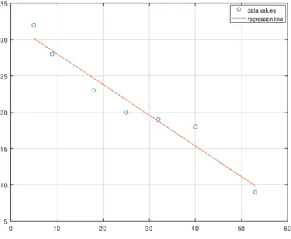
Now we plot a graph of this parabola together with our original data points. These are the commands used to create the graph:
>> x = l i n s p a c e( 0 , 7 , 5 0 ) ;
>> y = −0.89286*x . ˆ 2 + 5 . 6 5*x − 4 . 4 ;
>> p l o t( xdata , ydata , 'o', x , y , 'l i n e w i d t h', 2 )
>> g r i d on ;
>> l e g e n d('d a t a v a l u e s', 'l e a s t−s q u a r e s p a r a b o l a')
>> t i t l e('y = −0.89286 x ˆ2 + 5 . 6 5 x − 4 . 4')
The graph is shown in Figure 2.1.
You may be wondering if any of this process can be automated by built-in Octave functions. Yes! If we want Octave to do all of the work for us, we can use the built-in function for polynomial fitting, polyfit. The syntax is polyfit(x, y, order), where “order” is the degree of the polynomial desired.
Figure 2.2: Plot of original data vs. polyfit data
row vector. For example, [2 −3 4] corresponds to 2x2 −3x+ 4. The polyval function can be used to evaluate an Octave-format polynomial using the syntaxpolyval(P, x).
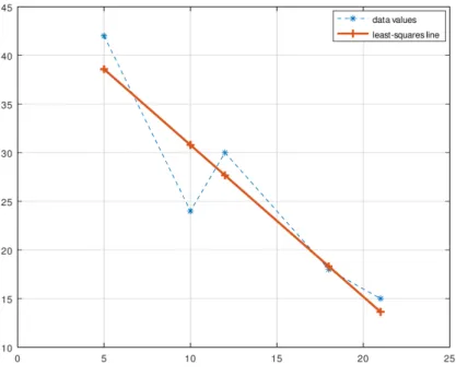
Example 2.2.2. Use polyfit to find the least-squares parabola for the following data:
x 1 2 3 4 5 6 y 1 2 5 4 2 -3
Graph the original data and polyfit data together on the same axes.
Solution. This is the same data as in Example2.2.1. Re-enter the data values if necessary.
We use polyfit to determine the equation, then thepolyval function to evaluate the polyno-mial at the given x-values.
>> P = p o l y f i t( xdata , ydata , 2 ) % d e g r e e two p o l y n o m i a l f i t
P =
−0.89286 5 . 6 5 0 0 0 −4.40000
>> y = p o l y v a l(P , xdata ) ; % e v a l u a t e p o l y n o m i a l P a t i n p u t xdata
>> p l o t( xdata , ydata , 'o−', xdata , y , '+−') ;
>> g r i d on ;
>> l e g e n d('o r i g i n a l d a t a', 'p o l y f i t d a t a') ;
-6
t t
t
t
t
@ @
@ @
@
1 2 3 4 5
1 2 3
Figure 2.3: House graph
2.3
Matrix transformations
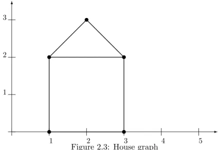
Matrices and matrix transformations play a key role in computer graphics. There are several ways to represent an image as a matrix. The approach we take here is to list a series of vertices that are connected sequentially to produce the edges of a simple graph. We write this as a 2×n
matrix where each column represents a point in the figure. As a simple example, let’s try to encode a “house graph.” First, we draw the figure on a grid and record the coordinates of the points, as in Figure2.3.
There are many ways to encode this in a matrix. An efficient method is to choose a path that traverses each edge exactly once, if possible1. Here is one such matrix, starting from (1,2) and traversing counterclockwise.
D=
1 1 3 3 2 1 3 2 0 0 2 3 2 2
Try plotting it in Octave and see if it worked.
>> D = [ 1 1 3 3 2 1 3 ; 2 0 0 2 3 2 2 ] D =
1 1 3 3 2 1 3
2 0 0 2 3 2 2
>> x = D( 1 , : ) ;
>> y = D( 2 , : ) ;
>> p l o t( x , y ) ;
You may want to zoom out to see the origin. Then the graph appears correct.
1
2.3.1 Rotation
Now that we have a representation of a digital image, we consider various ways to transform it. Rotations can be obtained using multiplication by a special matrix.
A rotation of the point (x, y) about the origin is given by
R· x y where R=
cos(θ) −sin(θ) sin(θ) cos(θ)
and θis the angle of rotation (measured counterclockwise).
For example, what happens to the point (1,0) under a 90◦ rotation?
cos(90◦) −sin(90◦) sin(90◦) cos(90◦)
· 1 0 = 0 −1 1 0 · 1 0 = 0 1
The rotation appears to work, at least in this case. Try a few more points to convince your-self. Notice that a rotation about the origin corresponds to moving along a circle, thus the trigonometry is fairly straightforward to work out.
Now, to produce rotations of a data matrix D, encoded as above, we only need to compute the matrix product RD.
Example 2.3.1. Rotate the house graph through 90◦ and 225◦.
Solution. Note that each θmust be converted to radians. Here we go:
>> D = [ 1 1 3 3 2 1 3 ; 2 0 0 2 3 2 2 ] ;
>> x = D( 1 , : ) ;
>> y = D( 2 , : ) ;
>> % e x e c u t e a 90 d e g r e e r o t a t i o n
>> t h e t a 1 = 90*p i/ 1 8 0 ;
>> R1 = [c o s( t h e t a 1 ) −s i n( t h e t a 1 ) ; s i n( t h e t a 1 ) c o s( t h e t a 1 ) ] ;
>> RD1 = R1*D;
>> x1 = RD1( 1 , : ) ;
>> y1 = RD1( 2 , : ) ;
>> % e x e c u t e a 225 d e g r e e r o t a t i o n
>> t h e t a 2 = 225*p i/ 1 8 0 ;
>> R2 = [c o s( t h e t a 2 ) −s i n( t h e t a 2 ) ; s i n( t h e t a 2 ) c o s( t h e t a 2 ) ] ;
>> RD2 = R2*D;
>> x2 = RD2( 1 , : ) ;
>> y2 = RD2( 2 , : ) ;
>> % p l o t o r i g i n a l and r o t a t e d f i g u r e s
Figure 2.4: Rotations of the house graph
>> a x i s([−4 4 −4 4 ] , 'e q u a l') ;
>> g r i d on ;
>> l e g e n d('o r i g i n a l ', 'r o t a t e d 90 deg', 'r o t a t e d 225 deg') ;
Note the combined plot options to set color, marker, and line styles. The original and rotated graphs are shown in Figure 2.4. Notice that the rotation is about the origin. For rotations about an arbitrary point, see Exercise14.
2.3.2 Reflection
If`is a line through the origin, then a reflection of the point (x, y) in the line` is given by
R·
x y
where
R=
cos(2θ) sin(2θ) sin(2θ) −cos(2θ)
andθ is the angle` makes with thex-axis (measured counterclockwise).
For example, what matrix represents a reflection in the liney=x? Here θ= 45◦.
cos(2·45◦) sin(2·45◦) sin(2·45◦) −cos(2·45◦)
=
cos(90◦) sin(90◦) sin(90◦) −cos(90◦)
=
0 1 1 0
Figure 2.5: Reflection of the house graph
What is the effect of this matrix on a point (x, y)?
0 1 1 0
·
x y
=
y x
We see that the point is indeed reflected in the liney=x.
Example 2.3.2. Reflect the house graph in the liney=x.
Solution. With the data matrix D and the original x and y vectors already defined, and using R as determined above, we have:
>> R = [ 0 1 ; 1 0 ] R =
0 1
1 0
>> RD = R*D;
>> x1 = RD( 1 , : ) ;
>> y1 = RD( 2 , : ) ;
>> p l o t( x , y , 'o−', x1 , y1 , 'o−')
>> a x i s([−1 4 −1 4 ] , 'e q u a l ') ;
>> g r i d on ;
>> l e g e n d('o r i g i n a l', 'r e f l e c t e d ')
Figure 2.6: Dilation of the house graph
2.3.3 Dilation
Dilation(i.e., expansion or contraction) can also be accomplished by matrix multiplication. Let
T =
k 0
0 k
Then the matrix productT D will expand or contract D by a factor of k.
Example 2.3.3. Expand the house graph by a factor of 2.
Solution. To scale by a factor of 2, we only need to multiplyDby the matrix
2 0 0 2
.
>> T = [ 2 0 ; 0 2 ] T =
2 0
0 2
>> TD = T*D;
>> x1 = TD( 1 , : ) ; y1 = TD( 2 , : ) ;
>> p l o t( x , y , 'o−', x1 , y1 , 'o−')
>> a x i s([−1 7 −1 7 ] , 'e q u a l') ;
>> g r i d on ;
>> l e g e n d('o r i g i n a l ', 'expanded')
2.3.4 Linear and nonlinear transformations
Rotation, reflection, and dilation are examples of linear transformations, and therefore can be represented as matrix products. However, not all of the graphical operations we are interested in are linear in this sense. In particular, translation is a nonlinear transformation which could instead be accomplished by matrix addition. But, in fact even a translation can be completed using a special kind of matrix product withhomogeneous coordinates. Refer to Exercises13–14
for some of the details and an example. This method preserves some of the properties of the linear transformations of the preceding sections.
If we use only multiplication for transformations, the composition of several transformations can be handled with the relatively simple operation of composing matrix multiplications. Fur-thermore, inverse transformations are easily produced by inverting the original transformation matrix2. For example, if T is a translation, R is a rotation, and S is a stretch, the combined operations of first translating, then rotating, then stretching can be completed with the matrix
SRT and a data matrixDcan be transformed with the product (SRT)D. The inverse of these combined operations is (SRT)−1 =T−1R−1S−1. Note that order matters!
2
Chapter
2
Exercises
1. Solve the system of equations using Gaussian elimination row operations
−x1+x2−2x3 = 1
x1+x2+ 2x3 = −1
x1+ 2x2+x3 = −2
To document your work in Octave, click “select all,” then “copy” under the edit menu, and paste your work into a Word or text document. After you have the row echelon form, solve the system by hand on paper, using backward substitution.
2. Use the multipliers from Exercise1to write an LU decomposition for
A=
−1 1 −2 1 1 2 1 2 1
Use this factorization to solve the systemAx=b, whereb=h−3,1,4i.
3. Consider the system of linear equationsAx=b, where
A=
1 −3 5 2 −4 3 0 1 −1
and b= 1 −1 3
Solve the system using left division. Then, construct an augmented matrixB and use rref to row-reduce it. Compare the results.
4. UseLU decomposition to solve the system from Exercise3. Use Octave’s [L U P] =lu(A) command. To useP A =LU to solve Ax =b, first multiply through by P, then replace
P AwithLU:
Ax = b
P Ax = Pb
LUx = Pb
SolveLy=Pb using forward substitution. Then solveUx=y using back substitution.
5. IfA is a singular matrix, Ax=b has no solutions or infinitely many solutions depending onb. How does Octave handle inconsistent systems, and in general, how does left division react to a singular coefficient matrix?
(a) To explore this question, let’s turn our previous system into an inconsistent one. Let
A and b be the matrices from Exercise 3. To construct an inconsistent system, we will make one row of the coefficient matrix into a linear combination of some other rows, without making the corresponding adjustment to the right-side constants. Do the following:
>> A( 1 , : ) = 3*A( 2 , : ) − 4*A( 3 , : )
(b) Now let’s consider a consistent system with infinitely many solutions. Keep A as above and make the corresponding adjustments to the right-side constants, yielding a system with infinitely many solutions.
>> b ( 1 , : ) = 3*b ( 2 , : ) − 4*b ( 3 , : )
Now solveAx=b using left division. Compare to the row-reduced echelon form.
The take away from these examples is that Octave will always give a solution when left division is used. If there are infinitely many solutions, a particular solution is given. If there are no solutions, Octave provides the least-squares (best-fitting) solution. It is always advisable to check the row-reduced echelon form of the coefficient matrix!
6. Octave can easily solve large problems that we would never consider working by hand. Let’s try constructing and solving a larger system of equations. We can use the command rand(m, n) to generate anm×nmatrix with entries uniformly distributed from the interval (0,1). If we want integer entries, we can multiply by 10 and use the floor function to chop off the decimal.
Use this command to generate an augmented matrixM for a system of 25 equations in 25 unknowns:
>>M = f l o o r( 1 0*rand( 2 5 , 2 6 ) ) ;
Note the semicolon. This suppresses the output to the screen, since the matrix is now too large to display conveniently. Solve the system of equations using rref and/or left division and save the solution as a column vectorx.
7. Consider the following data.
x 2 3 5 8
y 3 4 4 5
(a) Set up and solve the normal equations by hand to find the line of best fit, iny =mx+b
form, for the given data. Check your answer using polyfit(x, y, 1).
(b) Compare to the solution found using Octave’s left division operation directly on the relevant (inconsistent) system:
2 1 3 1 5 1 8 1 · m b = 3 4 4 5
(c) Plot a graph showing the data points and the regression line.
8. Use following commands to generate a randomized sample of 21 evenly spaced points from
x = 0 to x = 200 with a high degree of linear correlation. We start with a line through the origin with random slopem, then add some “noise” to eachy-value.
>> m = 2*rand − 1
>> x = [ 0 : 10 : 2 0 0 ]'
Use the polyfit function to find the least squares regression line for this data. Plot the data and the best-fitting line on the same axes. Run the simulation several times, then save two example plots which exhibit greater and lesser amounts of variation from the line
y=mx.
9. On July 4, 2006, during a launch of the space shuttle Discovery, NASA recorded the following altitude data3.
Time (s) Altitude (ft)
0 7
10 938
20 4,160 30 9,872 40 17,635 50 26,969 60 37,746 70 50,548 80 66,033 90 83,966 100 103,911 110 125,512 120 147,411
(a) Find the quadratic polynomial that best fits this data. Use Octave to set-up and solve the normal equations. After you have the equations set up, solve using either the rref command or the left-division operator.
(b) Plot the best-fitting parabola together with the given data points. Save or print the plot. Your plot should have labeled axes and include a legend.
(c) Use the first and second derivatives of the quadratic altitude model from part (a) to determine models for the vertical component of the velocity and acceleration of the shuttle. Estimate the velocity two minutes into the flight.
10. There are many situations where the polynomial models we have considered so far are not appropriate. However, sometimes we can use a simple transformation to linearize the data. For example, if the points (x, y) lie on an exponential curve, then the points (x,lny) should lie on a straight line. To see this, assume thaty=Cekx and take the logarithm of both sides of the equation:
y = Cekx
lny = lnCekx
= lnC+ lnekx = kx+ lnC
Make the change of variablesY = lny and A= lnC. Then we have a linear function of the form
Y =kx+A
3
We can find the line that best fits the (x, Y)-data and then use inverse transformations to obtain the exponential model we need:
y=Cekx
where
C =eA
Consider the following world population data4:
x= year y= population (in millions) Y = lny
1900 1650 7.4085
1910 1750
1920 1860
1930 2070
1940 2300
1950 2525
1960 3018
1970 3682
1980 4440
1990 5310
2000 6127
2010 6930
(a) Fill in the blanks in the table with the values for lny. Note that in Octave, the log(x) command is used for the natural logarithm. Make a scatter plot of x vs. Y. This is called a semi-log plot. Is the trend approximately linear?
(b) Use the polyfit function to find the best-fitting line for the (x, Y)-data and add the graph of the line to your scatter plot from part (a). Save or print the plot. Your plot should have labeled axes and include a legend. Note that the vertical axis is the logarithm of the population. Give the plot the title “Semi-log plot.”
(c) Use the data from part (b) to determine the exponential modely =Cekx. Plot the original data and the exponential function on the same set of axes. Save or print the plot. Your plot should have labeled axes and include a legend. Give the plot the title “Exponential plot.”
(d) Use the model from part (c) to estimate the date when the global population reached 7 billion.
(e) Make a projection about when the global population will reach 10 billion.
11. Create a data matrix that corresponds to a picture of your own design, containing six or more edges. Plot it.
(a) Rotate the image through 45◦ and 180◦. Plot the original image and the two rotations on the same axes. Include a legend.
(b) Expand your figure by a factor of 2, then reflect the expanded figure in the x-axis. Plot the original image, the expanded image, and the reflected expanded image on the same axes. Include a legend.
4
12. Let f(x) = x2, where −3 ≤ x ≤ 3. Use a rotation matrix to rotate the graph of the function through an angle of 90◦. Plot the original and rotated graphs on the same axes. Include a legend.
13. Let the point (x, y) be represented by the column vector
x y 1
. These are known as
homogeneous coordinates. Then the translation matrix
T =
1 0 h
0 1 k
0 0 1
is used to move the point (x, y) to (x+h, y+k) as follows:
1 0 h
0 1 k
0 0 1
· x y 1 =
x+h y+k
1
Use a translation matrix and homogeneous coordinates to shift the graph you created in problem11 as follows: shift 3 units left and 2 units up.
14. The translation method described in problem 13can be combined with a rotation matrix to give rotations around an arbitrary point. Suppose for example that we wished to rotate the house graph from Figure2.3about the center of the rectangular portion (coordinates (2,1) in the original figure). This can be done by using homogeneous coordinates and a translation T to move the figure, then a rotation matrix R for the rotation. The form of
R is now
R=
cos(θ) −sin(θ) 0 sin(θ) cos(θ) 0
0 0 1
Single variable calculus
3.1
Limits, sequences, and series
Octave is an excellent tool for many types of numerical experiments. Octave is a full-fledged programming language supporting many types of loops and conditional statements. However, since it is a vector-based language, some things that would be done using loops in Fortran or other traditional languages can be “vectorized.” As an example, let’s construct some numerical evidence to determine the value of the following limit:
lim n→∞
1 +1
n
n
We need to evaluate the expression for a series of larger and larger n-values. Here is what we mean by vectorized code: Instead of writing a loop to evaluate the function multiple times, we will generate a vector of input values, then evaluate the function using the vector input. This produces code that is easier to read and understand, and executes faster, due to Octave’s underlying efficient algorithms for matrix operations.
First, we need to define the function. There are a number of ways to do this. The method we use here is known as an anonymous function. This is a good way to quickly define a simple function.
>> f = @( n ) ( 1 + 1 . / n ) . ˆ n ; % anonymous f u n c t i o n
Note the use of elementwise operations1. We have named the function f. The input variable is designated by the @-sign followed by the variable in parentheses. The expression that follows gives the rule to be used when the function is evaluated. Now we can evaluate f at a single input value, or for an entire vector of input values.
Next, we create an index variable, consisting of the integers from 0 to 9.
1Elementwise operations are used throughout this chapter, since we are primarily evaluating functions element-wise at a numeric input vector, not doing matrix operations. Refer to Section1.4.1.
>> k = [ 0 : 1 : 9 ]' % i n d e x v a r i a b l e
k =
0 1 2 3 4 5 6 7 8 9
The syntax [0 : 1 : 9] produces a row vector that starts at 0 and increases by an increment of 1 up to 9. If not otherwise specified, the default step size is 1, so we could write simply [0 : 9]. Notice that we have used the transpose operation, only because our results will be a little easier to read as column vectors. Now, we’ll take increasing powers of 10, which will be the input values, then evaluate f(n).
>> f o r m a t l o n g % d i s p l a y a d d i t i o n a l d e c i m a l p l a c e s
>> n = 1 0 . ˆ k % s e q u e n c e o f i n c r e a s i n g i n p u t v a l u e s
n =
1 10 100 1000 10000 100000 1000000 1 0 0 0 00 0 0 1 0 0 0 0 0 0 0 0 1 0 0 0 0 0 0 0 0 0
>> f ( n ) % s e q u e n c e o f f u n c t i o n v a l u e s
ans =
2 . 0 0 0 0 0 0 0 0 0 0 0 0 0 0 2 . 5 9 3 7 4 2 4 6 0 1 0 0 0 0 2 . 7 0 4 8 1 3 8 2 9 4 2 1 5 3 2 . 7 1 6 9 2 3 9 3 2 2 3 5 5 2 2 . 7 1 8 1 4 5 9 2 6 8 2 4 3 6 2 . 7 1 8 2 6 8 2 3 7 1 9 7 5 3 2 . 7 1 8 2 8 0 4 6 9 1 5 6 4 3 2 . 7 1 8 2 8 1 6 9 3 9 8 0 3 7 2 . 7 1 8 2 8 1 7 8 6 3 9 5 8 0 2 . 7 1 8 2 8 2 0 3 0 8 1 4 5 1
>> f o r m a t % r e t u r n t o s t a n d a r d 5−d i g i t d i s p l a y
This is good evidence that the limit converges to a finite value that is approximately 2.71828. . .
Similar methods can be used for numerical exploration of sequences and series, as we show in the following examples.
Example 3.1.1. Let
∞
X
n=2
an be the series whose nth term is an= 1
n(n+ 2). Find the first ten terms, the first ten partial sums, and plot the sequence and partial sums.
Solution. To do this, we will define an index vectornfrom 2 to 11, then calculate the terms.
>> n = [ 2 : 1 1 ]'; % i n d e x
>> a = 1 . / ( n .*( n + 2 ) ) % t e r m s o f t h e s e q u e n c e
a =
0 . 1 2 5 0 0 0 0 0 . 0 6 6 6 6 6 7 0 . 0 4 1 6 6 6 7 0 . 0 2 8 5 7 1 4 0 . 0 2 0 8 3 3 3 0 . 0 1 5 8 7 3 0 0 . 0 1 2 5 0 0 0 0 . 0 1 0 1 0 1 0 0 . 0 0 8 3 3 3 3 0 . 0 0 6 9 9 3 0
If we want to know the 10th partial sum, we need only type sum(a). If we want to produce the sequence of partial sums, we need to make careful use of a loop. We will use a for loop with indexi from 1 to 10. For eachi, we produce a partial sum of the sequencean from the first term to theith term. The output is a 10-element vector of these partial sums.
>> f o r i = 1 : 1 0
s ( i ) = sum( a ( 1 : i ) ) ;
end
>> s' % s e q u e n c e o f p a r t i a l sums , d i s p l a y e d a s a column v e c t o r
ans =
0 . 1 2 5 0 0 0 . 1 9 1 6 7 0 . 2 3 3 3 3 0 . 2 6 1 9 0 0 . 2 8 2 7 4 0 . 2 9 8 6 1 0 . 3 1 1 1 1 0 . 3 2 1 2 1 0 . 3 2 9 5 5 0 . 3 3 6 5 4
Finally, we will plot the terms and partial sums, for 2≤n≤11.
>> p l o t( n , a , 'o', n , s , '+')
>> g r i d on
>> l e g e n d('t e r m s', 'p a r t i a l sums')
Figure 3.1: Plot of a sequence and its partial sums
An advantage of using a language like Octave is that it is simple to determine the sum of many terms of a series. If the series is known to converge, this can help give an estimate for the sum.
Example 3.1.2. Find the sum of the first 1000 terms of the harmonic series.
1000
X
n=1 1
n
Solution. We only need to generate the terms as a vector, then take its sum. Recall that ending a command with a semicolon prevents the output from being displayed on screen, done here since our sequence is now much too long to display conveniently.
>> n = [ 1 : 1 0 0 0 ] ;
>> a = 1 . / n ;
>> sum( a )
ans = 7 . 4 8 5 5
This is of course not an estimate for the sum of the infinite series, since, by the integral test, we know the series diverges. However, we can explore just how slowly this particular series diverges. The first 1000 terms sum to only about 7.5. Let’s try adding more terms:
>> n = [ 1 : 1 e6 ] ; % u s i n g s c i e n t i f i c n o t a t i o n f o r upper l i m i t
>> a = 1 . / n ;
>> sum( a )
ans = 1 4 . 3 9 3
![Figure 1.3: Default graph of y = sin(x) on [0, 2π]](https://thumb-us.123doks.com/thumbv2/123dok_us/8187735.2170585/21.918.259.686.127.475/figure-default-graph-of-y-x-on-π.webp)