Research Article Dynamic Time- and Load-Based Preference toward Optimal Appliance Scheduling in a Smart Home

(1)

Research Article

Dynamic Time- and Load-Based Preference toward Optimal

Appliance Scheduling in a Smart Home

I. Hammou Ou Ali , M. Ouassaid , and M. Maarouﬁ

Engineering for Smart and Sustainable Systems Research Center, Mohammadia School of Engineers, Mohammed V University in Rabat, Rabat 11000, Morocco

Correspondence should be addressed to I. Hammou Ou Ali; [email protected]

Received 28 November 2020; Revised 27 December 2020; Accepted 2 January 2021; Published 13 January 2021

Academic Editor: Jos´e Domingo ´Alvarez

Copyright © 2021 I. Hammou Ou Ali et al. This is an open access article distributed under the Creative Commons Attribution License, which permits unrestricted use, distribution, and reproduction in any medium, provided the original work is properly cited.

In this paper, the household appliance scheduling based on the user predefined preferences is addressed. Previous works generally deal with this problem without integration of renewable energy sources (RESs) in smart home. The present paper proposes a new demand side management (DSM) technique considering time-varying appliance preferences and solar panel generation. The branch and bound (B&B) algorithm is developed based on three postulations that allow the time-varying preferences to be quantified in terms of time- and load-based features. Based on the input data including the load’s power rating, the absolute comfort derived from time- and load-preferences, the total energy available from the solar panels as well as the energy purchased from the utility grid, the (B&B) algorithm is run to generate the optimal energy consumption model that would give maximum comfort to the householder based on the mixed-integer linear programming (MILP) technique. To test the performance of the proposed mechanism, three scenarios are considered with local energy production and limited budget for purchasing the energy from the utility grid to cover the user needs. The simulation results reveal that the proposed DSM mechanism based on the MILP method offers maximum level of comfort for all the scenarios within the available energy limitation.

1. Introduction

To face today’s power system issues, changing the traditional grid by a smart one has become a necessity. Smart grid takes advantage of smart metering infrastructure, advanced communication technologies as well as intelligent control systems to keep the balance between the supply and the demand while ensuring a reliable communication between the utility grid and the end user [1, 2]. In this context, efforts at this time are oriented towards energy management according to two sides: supply side management (SSM) and demand side management (DSM) [3, 4]. The first category deals with efficient energy production, transmission, and distribution to the user at a low cost. However, DSM mainly relies on planning, controlling, and scheduling the use of the home appliances.

Since the main target behind DSM is to reduce the user’s electricity bills while guaranteeing the user comfort, several

DSM techniques and algorithms including artificial intelli-gence (AI) and optimization algorithms are used in the literature. AI has recently immersed in the field of DSM to tackle its various challenges, among the most used methods: artificial neuron network, multiagent system, machine learning, and nature-inspired AI [5]. However, the opti-mization algorithms are used to solve a mathematical problem. These algorithms are classified into deterministic methods such as linear programming (LP), nonlinear pro-gramming (NLP), and mixed-integer linear propro-gramming (MILP). However, the second class is about stochastic methods; it includes genetic algorithm (GA), tabu search, and particle swarm optimization [6].

In fact, home energy management (HEM) is gaining more attention in terms of scheduling the home appliances in order to achieve the DSM objectives. Among these, the critical objective is to maximize the user comfort at a pre-deﬁned available energy. Most of the research studies relate Volume 2021, Article ID 6640521, 16 pages

(2)

the comfort to static and dynamic preference choices assigned to the usage of the home appliances. The static preferences are time-independent where the user can at-tribute some preference level over a day. The appliances with a high preference level must operate the ﬁrst [7]. In dynamic preference, i.e., time-dependent preference, the user can modify his preference level with respect to time. For in-stance, a householder gives preference to the water heater in the morning, and at night, he changes its preference since he needed to have his shower at the same time in the morning [8].

Given the foregoing considerations of the user comfort in the ﬁeld of load energy management, the present work considers the user comfort according to time- and load-based preference to evaluate the user absolute comfort. The aim of the proposed load comfort management technique is to maximize the user comfort level at a predeﬁned available energy based on mixed-integer linear programming (MILP) technique. This study also develops available energy per unit comfort index (IAE/uc), which relates the total energy available (TEA) with the achieved comfort (AC).

1.1. Contributions. In the assessment of the previous re-search, this study proposed an exact method to solve the home appliance scheduling problem with user comfort. Moreover, absolute comfort based on time variation pref-erences with solar panel integration and daily budget lim-itation over a day is treated in this work. In time-based preference, time-varying preferences are assigned to an appliance by the user at diﬀerent time intervals in a day. In load-based preferences, the user assigns relative preference to the load in each operating time interval (OTI). It can change in various time intervals within a day. Thus, the main contributions of the present research work can be listed as follows:

(i) Dynamic user comfort model is used to solve the home appliance scheduling problem taking into account time- and load-based preferences. (ii) Mixed-integer linear programming (MILP)

tech-nique is developed to generate an optimal energy consumption model that would yield a high level of comfort to the user.

(iii) The proposed load comfort management scheme meets the energy constraints and the daily budget limitation under several scenarios with solar panel integration.

(iv) Available energy per unit comfort index which links between the total energy available from the solar panels and the utility grid and the total achieved comfort is taken into account in this work.

1.2. Paper Organization. The rest of this work is structured as follows. Section 2 discusses the literature review. Section 3 elaborates the concept of preference and presents the pro-posed system architecture. In Section 4, the propro-posed strategy and the used algorithm are presented. Section 5

deals with the results and discussion based on 3 scenarios. Section 6 concludes the work.

2. Literature Review

Since the 70s of the last century, several research papers are published in the field of DSM and up to now it still a trending topic. Authors in [9] discuss an experimental home appliance scheduling problem while considering the user’s predefined preferences. The proposed binary integer linear programming optimization (BILPO) model realizes efficient electricity cost saving in short computation time. However, reference [10] proposes a system architecture and a user-friendly algorithm for DSM with the use of information and communication technology (ICT). Tested under real data, the objective function was reached in terms of minimizing the electricity bills, the peak load, and maximizing the usage pattern. Authors in [11] propose a smart home controller (SHC) to manage the energy consumption in a residential sector with multiple households. The proposed model is formulated as a multiobjective mixed-integer linear pro-gramming (MOMILP) to take advantage of lower-cost pricing and at the same time reduce the peak demand. Another work in [12] considers high-power controllable loads in a house such as electric water heater, electric vehicle (EV), heating-ventilation, and air conditioning (HVAC) system. The aim of the proposed model is to optimize the electricity consumption cost based on traditional saving families and modern comfortable families. In [13], the authors address the residential appliance scheduling while considering the consumer’s preferences and the reduction of peak load. The problem is formulated as MOMILP, and the numerical experiments show that the proposed model can reduce significantly the electricity cost, the consumer inconvenience, and the peak load. In [14], the authors develop a hybrid technique combining the genetic algo-rithm (GA) with binary particle swarm optimization (BPSO) for residential load scheduling to minimize the energy consumption cost and the consumer comfort. The performance of the proposed model is evaluated in terms of electricity cost, peak to average ratio (PAR), and user discomfort. However, the authors in [15] develop a load scheduling algorithm based on cost efficiency and con-sumer’s preference to effectively reflect and affect user’s consumption behavior and achieve the optimal energy consumption profile. Tested under real data, the proposed method realizes the desired trade-off between economic efficiency and consumer’s preference. In the same context, authors in [16] propose a convex optimization problem for scheduling the home appliances under a day-ahead elec-tricity pricing. The proposed power scheduling strategy can achieve a trade-off between the user discomfort and the electricity payment. Similarly, the authors in [17] propose a fractional programming approach to schedule the electrical appliances in a smart house based on cost efficiency and consumer consumption preferences. Tested under four consumption models, the proposed method is proved to be efficient in improving the consumers’ consumption and satisfaction while saving costs.

(3)

Renewable energy and storage systems have been increasingly integrated in smart houses, which is the subject of several research studies. In [18], the authors propose a model with and without the integration of the renewable energy sources (RESs) to scheduling the home appliances. The proposed model reduces the peaks and the electricity bills using evolutionary algorithms (EAs) such as binary particle swarm optimization (BPSO), genetic algorithm (GA), and cuckoo search. The authors in [19] utilize a stochastic optimization approach to find the optimal schedules for a home energy management system (HEMS) where energy prices and generation from re-newable sources are time-varying. The aim of the pro-posed method is to find the minimum energy cost while taking into account the supply and demand constraints. To balance the residential load curve, the authors in [20] propose a system model based on the coordination of microgrids using a dynamic algorithm. The problem is formulated as a biobjective optimization problem, and the obtained results demonstrate the efficiency of the pro-posed approach in balancing the load curve. In [21], the authors evaluate the performance of a designed home energy management controller with RES integration based on GA and binary particle swarm optimization (BPSO) in terms of electricity bill reduction, peak to average ratio minimization, and user comfort level maximization. Therefore, the work in [22] proposes a strategy for residential community in smart grid that optimally schedules the home appliances using MILP. Without bringing the user discomfort, the proposed model reduces both the electricity cost and the peak load. With the integration of RESs and smart communication technology in a home, the work presented in [23] develops an intelligent home energy management which ensures effective utilization of the RESs and provides significant savings. Moreover, the work presented in [24] proposes a multiobjective model for managing the residential loads with solar panels and batteries integration. The proposed model proves its efficacy in reducing the user’s discomfort, the total electricity cost, and the standard deviation of the consumed power. A mixed-integer linear programming (MILP) model with solar panels and energy storage in-tegration is proposed in [25] to efficiently allocate the load consumption based on a predefined priority of the user’s loads.

With insight of the diﬀerent works discussed before, it can be concluded that the major challenges associated with DSM can be summarized in three main points: minimizing the electricity bills, the PAR, and the dis-comfort. Both, formal techniques and metaheuristics al-gorithms are vastly applied to solve the home appliance scheduling problem in an awe-inspiring way. The user comfort is a key indicator that reﬂects if the user is pleased or not with appliance usage. It depends on the preferences of the users which can vary from a user to another one. Static preferences assigned to the home appliances are commonly applied by the researchers. Incorporating dynamic preferences can better enhance user comfort. Most of the works in the literature associate the user

comfort with thermal comfort caused by the power de-viation and the delay caused by scheduling the appliance usage. However, the preference of the user is ignored which is the main target of this work.

3. Concept of Preference and the Proposed

Model Architecture

User preference is the main factor that influences the de-mand in several areas; it refers to whether the user is pleased or not with a certain product or service. In the field of home energy management, generally, the householder has dif-ferent types of appliances which demand different power rating to function. Moreover, these appliances have different preference levels that can vary from a user to another according to his situation and attitude throughout a day.

3.1. Preference Concept and Postulations. It is commonly known that the user’s main attention is to pay fewer bills while being comfortable. As proposed in this work, the user has a budget limitation to spend on his energy demand during one day. The real challenge involved in the home energy management controller (HEMC) is to determine the time and device usage pattern that may provide maximum comfort at limited energy available. In this concept, the index of available energy per unit comfort is introduced, and it can be expressed as follows:

I_AE/UC�TEA

TAC, (1)

where TEA is the total energy available from solar panels and utility grid according to the budget limitation and TAC is the total achieved comfort. Given that the user’s objective is to maximize TAC while keeping TEA ﬁxed; hence,IAE/UCmust be the minimum possible. To achieve that target, the fol-lowing postulations are made:

(i) The preferencep is quantiﬁed and can be numer-ically evaluated.

(ii) The preferenceptakes values in between complete preferencep�1 and complete indiﬀerencep�0. (iii) The preference is relative and comparative. The two

preference levels are deﬁned as load-based and time-based preference.

In time-based relativity, the preference assigned to an appliance#Ichanges with respect to diﬀerent time intervals during the day. If there is an appliance #I, then the pref-erence set by the householder in timet1can be represented as (pI(t1)).This preference is relative, and it can be compared with the preference it provides at time t2 (pI(t2)).

In load-based relativity, if two appliances #I and #J operate at the same time t1, (pI(t1)) and (pJ (t1)) can be compared. For example, at 13 pm if the user is hungry and wants to turn on the microwave and at the same time the washing machine but he is under an energy constraint which forbids him from using both. In this situation, he attributes high value to the appliance with the highest preference.

(4)

3.2. System Model Architecture of Smart Home. Figure 1 demonstrates a graphical representation of the proposed model that performs for scheduling the home appliances. It consists of integrating solar panels and power grid to cover the user energy needs. The proposed smart home is com-posed of 5 sections; each section is equipped with multiple devices. The specification of the appliances is detailed in Table 1. It is worth mentioning that the electricity tariff (ET) received from the utility thought the smart meter (SM) is fixed at 0.115$/kWh. This ET is used to estimate the total energy available (TEA) at a fixed budget. However, based on daily temperature and solar irradiance, the total energy available from solar panels can be obtained as shown in Figure 2. In case of surplus energy production, the user can sell the energy to the grid utility at the same tariff of 0.115$/ kWh. Through the user interface, the householder can evaluate his preferences based on time relativity and load relativity. The challenge of the home energy management controller (HEMC) is to find the optimal model for the energy consumption of the home appliances to yield maximum comfort to the user under the energy constraint limitations. Advanced communication protocols are in-stalled at home to ensure the communication between the HEMC, SM, and the appliances. Among the various tech-nologies existing in the market, Wi-Fi, Bluetooth, and Z-Wave provide reliable communication at a low cost [26]. 3.3. Absolute Comfort. In this work, the absolute comfort results from the time-based table preference and the load-based table preference assigned to the user to fill in with values between 0.0 and 1.0. The input data (i.e., time-based preference and load-based preference) are transmitted from the user interface (UI) to the home energy management controller (HEMC) to calculate the absolute comfort as discussed later on.

3.3.1. Time-Based Preference Table. In the time-based preference table, the householder ﬁlls in each box of the table horizontally as follows:

(i) The user takes an appliance#Iand decides in which hour of the daytmax its usage is highest.

(ii) A maximum preference value is attributed to this hour (tmax),pI(tmax)�1.

(iii) For the rest of the day, the user compares his preference from the use of the appliance #I and assigns values between the highest preference level 1.0 and lowest preference level 0.0 as expressed in the following:

0≤p_I(t)≤1, ∀t� [1,24]. (2)

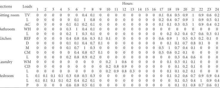
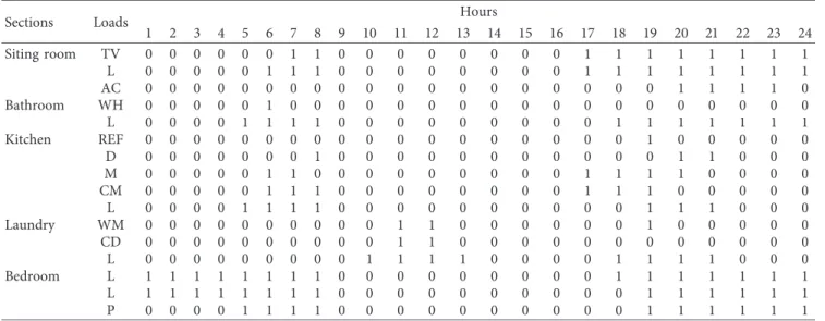
The previous actions must be repeated for all the con-sidered appliances all over 24 hours. This process is more explained in Figure 3. Table 2 shows the time-based pref-erence table ﬁlled by a typical householder. It is noted that these data can be changed according to each user. Here, it can be depicted from Table 2 that the householder attributes

maximum time-based preference to TV in time intervals 20 and 21 because it is time for daily news; however, at time 22, 23, and 24, his preference decreases to 0.9, 0.5, and 0.2, respectively; this is based on the second postulate (prefer-ences are comparable).

3.3.2. Load-Based Preference Table. In load-based prefer-ence table, the data are ﬁlled vertically by the householder following the next steps:

(i) The householder chooses a speciﬁc hourt. (ii) If the appliances#I,#J, and#Kare available to be

used, then the user sets the maximum preference to an appliance#Ibecause of its maximum utility at that time hourt,pI(t)�1.

(iii) The rest of the appliances are compared with this reference device#Iand take values from 0.0 to 1.0. Table 3 shows the load-based preference table of the considered user in this work. It can be seen from the table that at time interval 21, the maximum load-based preference value 1 is assigned to TV, lighting, AC, and phone charger. It indicates that the householder expects using all those ap-pliances at 21 h. The rest of the apap-pliances take relative preferences with respect to this maximum preference value. 3.3.3. Absolute Comfort. The absolute comfort takes into consideration the two-input data (time-based and load-based preference). The absolute comfort of an appliance#Iat time tiis calculated as follows [27]:

ACI(t) � �� pT_I(t)2+pL_I(t)2 􏽱 � 2 √ , (3) wherepT

I(t)andpLI(t)are, respectively, the time-based and

load-based preference of an appliance #I at time t. For normalization purposes, a denominator of √�2 is used. So, the AC will take values between 0 and 1. For example, Table 2 reveals that the time-based preference value of the micro-wave at 6 h is equal to 0.8. However, the load-based pref-erence at the same time in Table 3 indicates a value of 0.5. Using equation (3), the absolute comfort of the microwave can be calculated as follows:

CI ti􏼁� �� 0.82+0.52 􏽰 � 2 √ _≈_0.7. (4)

For all the appliances during 24 hours, the absolute comfort obtained using equation (3) is represented in Table 4.

4. Proposed Load Comfort Management

Strategy and the Used Algorithm

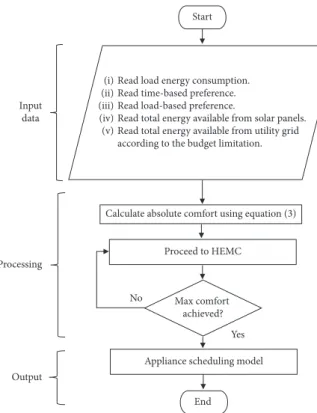
The proposed load comfort management strategy is com-posed of three main segments, namely, the input, the process, and the output as shown in Figure 4. The input data include the loads power ratings, the time-based preference, the load-based preference, the total energy available from the

(5)

solar panels, and the utility grid according to the budget limitation. The HEMC calculates the absolute comfort and ﬁnds the optimal scheduling model of the appliances that give maximum comfort which is the output data. The computing method is elaborated hereafter using mixed-integer linear programming (MILP) technique. The detailed process of the proposed strategy is explained in Figure 4.

4.1. Objective Function. The objective of the proposed technique is to schedule the home appliances in such a way the user comfort is maximized at a ﬁxed budget. As it can be observed from equation (1), the available energy per unit comfort IAE/UCis a function of the total available energy TEA and the user’s comfort UC. Hence, the objective function can be rewritten as follows:

Sitting room Bedroom Kitchen Bathroom Laundry HEMC UI SM Grid RES Electrical switch

Figure1: System model architecture of the proposed smart home.

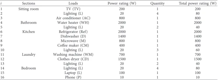
Table1: Load energy consumption.

i Sections Loads Power rating (W) Quantity Total power rating (W)

1 Sitting room TV (TV) 200 1 200

2 Lighting (L) 20 4 80

3 Air conditioner (AC) 800 1 800

4 Bathroom Water heater (WH) 2000 1 2000

5 Lighting (L) 20 2 40

6 Kitchen Refrigerator (Ref ) 2000 1 2000

7 Dishwasher (D) 1400 1 1400

8 Microwave (M) 800 1 800

9 Coﬀee maker (CM) 400 1 400

10 Lighting (L) 20 3 60

11 Laundry Washing machine (WM) 700 1 700

12 Clothes dryer (CD) 1500 1 1500

13 Lighting (L) 20 2 40

14 Bedroom Lighting (L) 20 4 80

15 Laptop (L) 100 1 100

(6)

4 6 8 10 12 14 16 18 20 22 24 2 Time (hours) 0 500 1000 1500 2000 2500 Ener g y g enera tio n (W h) Day of December Day of July

Figure2: Renewable energy generation from solar panels in Rabat city in Morocco.

Start

Pick an appliance #I

Assign preference value of 1 to t_max

Initialize times slot index t = 1

t = 24 t = _t+ 1 Any appliance left? End Yes No Yes No

Select t_max where that appliance utility is highest

Assign preference value to t in comparison to _p_I (_t_max)

Figure3: Flow-chart of the time-based preference table.

Table2: Time-based preference table.

Sections Loads Hours

1 2 3 4 5 6 7 8 9 10 11 12 13 14 15 16 17 18 19 20 21 22 23 24 Sitting room TV 0 0 0 0 0 0 0.2 0.1 0 0 0 0 0 0 0 0 0 0.4 0.5 1 1 0.9 0.5 0.2 L 0 0 0 0 0 0.2 1 0.8 0 0 0 0 0 0 0 0 0 0.3 0.8 1 1 0.9 0.4 0.1 AC 0 0 0 0 0 0.1 0.2 0 0 0 0 0 0 0 0 0 0 0.1 0.3 0.5 1 1 0.5 0.3 Bathroom WH 0 0 0 0 0.3 1 0.5 0.1 0 0 0 0 0 0 0 0 0 0 0 0 0 0 0 0 L 0 0 0 0 0.2 1 0.4 0.1 0 0 0 0 0 0 0 0 0 0.1 0.2 0.2 1 0.8 0.4 0.1

(7)

Table2: Continued.

1 2 3 4 5 6 7 8 9 10 11 12 13 14 15 16 17 18 19 20 21 22 23 24 Kitchen REF 0 0 0 0 0.5 1 0.7 0.4 0.1 0.2 0 0 0 0 0 0 0.1 0.9 1 0.5 0.3 0.2 0.1 0 D 0 0 0 0 0.1 0.1 0.5 1 0.1 0 0 0 0 0 0 0 0 0 0.1 0.2 1 0.1 0 0 M 0 0 0 0 0.1 0.8 1 0.4 0 0 0 0 0 0 0 0 0.3 1 0.8 0.4 0 0 0 0 CM 0 0 0 0 0 0 0.6 1 0.2 0 0 0 0 0 0 0 0.3 0.9 0.3 0 0 0 0 0 L 0 0 0 0 0.3 1 0.7 0.3 0 0 0 0 0 0 0 0 0 0 0.1 0.5 0.8 0 0 0 Laundry WM 0 0 0 0 0 0 0 0 0 0.3 1 0.8 0 0 0 0 0 0.1 0.4 0 0 0 0 0 CD 0 0 0 0 0 0 0 0 0 0.3 1 0.7 0 0 0 0 0 0 0.1 0.3 0 0 0 0 L 0 0 0 0 0 0 0 0 0 0.3 1 1 0.5 0 0 0 0 0.2 0.2 0.2 0 0 0 0 Bedroom L 0 0 0 0 0.4 1 0.7 0.4 0 0 0 0 0 0 0 0 0 0.1 0.3 0.8 0.9 1 0.8 0.5 L 0 0 0 0 0.2 0.5 0.3 0.1 0 0 0 0 0 0 0 0 0 0 0 0.7 0.5 1 1 0.4 P 0 0 0 0 0.8 1 0.5 0 0 0 0 0 0 0 0 0 0 0 0 0 0.4 0.7 0.8 0

Table3: Load-based preference table.

1 2 3 4 5 6 7 8 9 10 11 12 13 14 15 16 17 18 19 20 21 22 23 24 Sitting room TV 0 0 0 0 0 0 0.5 0.2 0 0 0 0 0 0 0 0 0.2 0.4 0.6 0.8 1 1 0.7 0.2 L 0 0 0 0 0 0.1 1 0.8 0 0 0 0 0 0 0 0 0.3 0.5 0.6 0.7 1 0.9 0.6 0.1 AC 0 0 0 0 0.1 0.2 0.3 0.1 0 0 0 0 0 0 0 0 0.2 0.2 0.3 0.6 1 0.9 0.4 0.1 Bathroom WH 0 0 0 0 0.3 1 0.2 0.1 0 0 0 0 0 0 0 0 0 0 0 0 0 0 0 0 L 0 0 0 0 0.3 1 0.1 0.1 0 0 0 0 0 0 0 0 0 0.3 0.3 0.5 0.2 0 0 0.1 Kitchen REF 0 0 0 0 0.2 0.6 0.4 0.1 0 0 0 0 0 0 0 0 0.8 0.9 1 0.5 0.3 0.2 0.1 0 D 0 0 0 0 0 0.1 0.1 0 0 0 0 0 0 0 0 0 0 0.1 0.2 1 0.6 0.2 0 0 M 0 0 0 0 0 0.5 1 0.1 0 0 0 0 0 0 0 0 0.7 1 0.6 0.4 0.2 0 0 0 CM 0 0 0 0 0 0.6 1 0.1 0 0 0 0 0 0 0 0 0.7 0.1 0.1 0.1 0 0 0 0 L 0 0 0 0 0.1 0.5 1 0.2 0 0 0 0 0 0 0 0 0 0 0.4 0.2 0.1 0 0 0 Laundry WM 0 0 0 0 0 0 0 0 0 0 1 0.3 0 0 0 0 0 0 0.2 0.2 0.2 0 0 0 CD 0 0 0 0 0 0 0 0 0 0 0.4 1 0 0 0 0 0 0 0.2 0.2 0.2 0 0 0 L 0 0 0 0 0 0 0 0 0 0 0.4 0.5 0 0 0 0 0 0 0.1 0.2 0.2 0 0 0 Bedroom L 0.2 0.2 0.2 0.2 0.3 0.4 0.3 0.2 0 0 0 0 0 0 0 0 0 0.1 0.2 0.1 0.3 0.7 0.1 0.3 L 0.1 0.1 0.1 0.1 0.3 0.3 0.2 0.1 0 0 0 0 0 0 0 0 0 0 0.1 0.1 0.2 1 0.8 0.5 P 0 0 0 0 0 0.5 0.6 0.1 0 0 0 0 0 0 0 0 0 0 0.1 0.1 1 0.8 0.2 0.1

Table4: Absolute comfort table.

1 2 3 4 5 6 7 8 9 10 11 12 13 14 15 16 17 18 19 20 21 22 23 24 Sitting room TV 0 0 0 0 0 0 0.4 0.1 0 0 0 0 0 0 0 0 0.1 0.4 0.5 0.9 1 0.9 0.6 0.2 L 0 0 0 0 0 0.1 1 0.8 0 0 0 0 0 0 0 0 0.2 0.4 0.7 0.9 1 0.9 0.5 0.1 AC 0 0 0 0 0.1 0.1 0.2 0.1 0 0 0 0 0 0 0 0 0.1 0.1 0.3 0.5 1 0.9 0.4 0.2 Bathroom WH 0 0 0 0 0.3 1 0.4 0.1 0 0 0 0 0 0 0 0 0 0 0 0 0 0 0 0 L 0 0 0 0 0.2 1 0.3 0.1 0 0 0 0 0 0 0 0 0 0.2 0.2 0.4 0.7 0.6 0.3 0.1 Kitchen REF 0 0 0 0 0.4 0.8 0.6 0.3 0.1 0.1 0 0 0 0 0 0 0.6 0.9 1 0.5 0.3 0.2 0.1 0 D 0 0 0 0 0.1 0.1 0.4 0.7 0.1 0 0 0 0 0 0 0 0 0.1 0.1 0.7 0.8 0.1 0 0 M 0 0 0 0 0.1 0.7 1 0.3 0 0 0 0 0 0 0 0 0.5 1 0.7 0.4 0.1 0 0 0 CM 0 0 0 0 0 0.4 0.8 0.7 0.1 0 0 0 0 0 0 0 0.5 0.6 0.2 0.1 0 0 0 0 L 0 0 0 0 0.2 0.8 0.9 0.2 0 0 0 0 0 0 0 0 0 0 0.3 0.4 0.6 0 0 0 Laundry WM 0 0 0 0 0 0 0 0 0 0.2 1 0.6 0 0 0 0 0 0.1 0.3 0.1 0.1 0 0 0 CD 0 0 0 0 0 0 0 0 0 0.2 0.8 0.9 0 0 0 0 0 0 0.1 0.2 0.1 0 0 0 L 0 0 0 0 0 0 0 0 0 0.2 0.9 0.8 0.3 0 0 0 0 0.1 0.1 0.2 0.1 0 0 0 Bedroom L 0.1 0.1 0.1 0.1 0.3 0.8 0.5 0.3 0 0 0 0 0 0 0 0 0 0.1 0.2 0.6 0.7 0.9 0.9 0.4 L 0.1 0.1 0.1 0.1 0.2 0.4 0.2 0.1 0 0 0 0 0 0 0 0 0 0 0.1 0.5 0.4 1 0.9 0.4 P 0 0 0 0 0.6 0.8 0.5 0.1 0 0 0 0 0 0 0 0 0 0 0.1 0.1 0.8 0.7 0.6 0.1

(8)

Obj I_AE/uc􏼁�min I_AE/UC􏼁. (5) The total energy available is a summation of energy available from the solar panels and the energy purchased from the utility grid:

TEA�TEAPV+TEAGrid, (6)

where TEAPVis the total energy available produced locally by the solar panels. Knowing the daily temperature and solar irradiation, the TEAPVcan be obtained as follows:

TEAPV �􏽘 24 t�1 ηPV×APV×I t r 1−0.005 T t a−25 􏼐 􏼑 􏼐 􏼑 􏼐 􏼑, (7)

where ηPV is the energy conversion eﬃciency of the solar panel system,A_PVis the array of the generator,It_ris the solar irradiance (kW/m2), andTt

ais the outdoor temperature (°C).

TEAgrid is the energy obtained from the utility grid. Knowing the budget limitation B, the TEAgrid can be cal-culated as follows:

TEAGrid� B

ET, (8)

where Bis the daily budget and ET is the electricity tariﬀ.

4.2. Mapping the Comfort Scheduling Model. Similar to the overall approaches to the solution of the constraint opti-mization problems, the branch and bound (B&B) algorithm has been established as an intelligent computational tool for solving integer programming, nonlinear programming, traveling salesman, and quadratic assignment [28]. The B&B

algorithm searches the complete space of solutions to a given problem for the best exact solution. B&B is based on the observation that the enumeration of integer solutions has a tree structure, and the main idea in B&B is to avoid growing the whole tree as much as possible because the entire tree is too big for real problems. In this work, the problem model is formulated as a mixed-integer linear programming with binary decision variables 0-1. The computing steps are followed to ﬁnd out the optimal scheduling model: (Algorithm 1)

5. Results and Discussion

In order to scrutinize the performance of the proposed load comfort management technique, several scenarios are studied in this section based on the daily energy available from the solar panels as well as the user’s daily budget limitation. From the desired comfort and the load energy consumption table, the proposed technique is run to ﬁnd time interval where allocating energy so as to achieve maximum comfort at every budget limitation. The following sections establish the analysis of the results obtained from the three scenarios.

5.1. Scenario 1: Considering Just Solar Panel Generation. In this scenario, only solar panels are used to meet up the household energy needs. Connected with the grid, the solar panels allow the injection of the energy produced in order to bring the necessary energy when required. Since the energy produced from the solar panel is not the same all over the year, in this work we suppose a typical day in December and

Read load energy consumption. Read time-based preference. Read load-based preference.

Read total energy available from solar panels. Read total energy available from utility grid according to the budget limitation. (i)

(ii) (iii) (iv) (v)

Calculate absolute comfort using equation (3)

Proceed to HEMC

Max comfort achieved?

Appliance scheduling model

End Yes No Input data Processing Output Start

(9)

July in Rabat city in Morocco. Figure 2 represents the daily energy generation from the solar panels.

The aim of this proposed load comfort management technique is to determine the energy consumption model that would allow maximum comfort to the householder at the same quality of energy produced locally. The obtained results for the two cases are presented in Tables 5 and 6, respectively. The value of 1 indicates that the corresponding appliance must be turned ON at that time interval while the value of 0 enforces the load to be turned OFF.

The performance of the proposed algorithm for this scenario is depicted in Table 7. The total energy available from the solar panels is assumed to be 14.295 kWh in the day of December; however, for the day of July, it is assumed to be 21.81 kWh. From Table 4, the total desired comfort (TDC) is obtained by summing all the user’s absolute comfort input for all the considered appliances during the day. It can be expressed as follows: TDC�􏽘 24 t�1 􏽘 N i�1 AC(i, t), (9)

where trepresents time interval during one day and i de-notes the home appliances. Moreover, the total achieved comfort (TAC) is obtained by adding the user’s absolute comfort value outputs derived from Table 5 and Table 6 according to each considered case. The level of comfort (LOC) is the ratio of the TAC to the TDC. It can be cal-culated as follows:

LOC %�TAC

TDC. (10)

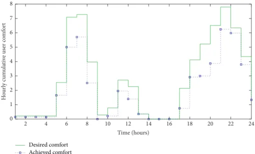
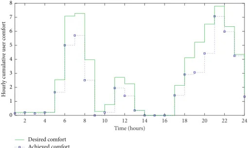
Table 7 brings out the performance of the proposed technique for the two cases. For the day in December, the LOC is estimated as 71.4267%. However, in the day of July,

the LOC achieves 78.21%. The comparison between the hourly desired comfort and achieved comfort for the two cases is shown in Figures 5 and 6, respectively.

The total operating time (TOT) value of all the ap-pliances in the ﬁrst scenario is given in Table 8. It can be observed that some energy consuming devices like the dish washer and the cloth dryer start operating in the July day. Moreover, other appliances have increased their operating time such as TV, air conditioner, microwave, and laptop which justify the increase value of LOC in the day of July.

5.2. Scenario 2: Considering a Budget Limitation of 0.5$/Day. In this scenario, both solar panels and energy grid are used. A budget limitation of 0.5$/day is considered. Same as the previous scenario, the proposed load comfort management technique is performed in order to obtain maximum comfort according to this budget limitation for the two cases, i.e., a day of December and a day of July. The load allocation patterns obtained for the two cases are shown in Tables 9 and 10, respectively.

Table 11 represents the obtained results for the two cases. It is obviously known that an increase in the total energy available will immediately increase the LOC. Its value is getting higher when compared with scenario 1 while con-sidering the same cases. The highest value of LOC is 81.51% on the day of July. Meanwhile, in December, the LOC has increased from 71.4267% in the previous scenario to 75.5413% in the current one. Besides, theIAE/UCindex is also higher in case of July day, i.e., 0.48 because the HEMC can aﬀord consumption of high-power rated loads which were kept OFF in the previous scenario. Another justiﬁcation of the increase in theIAE/UCindex is that the appliances may be operated for a long period of time.

(1) Start procedure

(2) Input data: load energy consumption table, time-based preference table, load-based preference table, budget, and TEAPV. (3) Compute absolute comfort using equation (3), TEAPVusing equation (7), and TEAGridusing equation (8).

(4) Fori�1 tondo (5) Fort�1 to 24 do

(6) Evaluate the following optimization expression:

Max 􏽘24_t_�₁􏼠 􏽘 n i�1 AC(i, t) ×x(i, t)􏼡 S.t. 􏽘24_t_�₁􏼠 􏽘 n i�1

P(i, t) ×x(i, t)􏼡≤TEAPV+TEAGrid

􏽘24 t�1􏼠 􏽘 n i�1 x(i, t)􏼡≤δ x(i, t) � 0 1 􏼨 ⎧ ⎪ ⎪ ⎪ ⎪ ⎪ ⎪ ⎪ ⎪ ⎪ ⎨ ⎪ ⎪ ⎪ ⎪ ⎪ ⎪ ⎪ ⎪ ⎪ ⎩ where AC is the

absolute comfort matrix,Pis the appliance power matrix,δrepresents the length of the boxes where the user’s absolute comfort is diﬀerent from 0, andxis the decision variable output, and it takes 0/1 if the load is OFF/ON.

(7) End for

(8) End for

(9) Returnx(i,t) the decision variable output (10) Calculate the level of comfort using equation (10) (11) End procedure

(10)

At the same budget limitation, the TOT of all the appli-ances in the second scenario is given in Table 12. As a com-parison between the previous case and the current one in the case of a December day, it can be seen that the TOT of several appliances has increased other appliance like the dish washer which has been switched OFF in scenario 1 start operating in this scenario. Moreover, in the case of July day appliances like the water heater and the refrigerator start operating for the ﬁrst time and other appliances are used for a long period.

Figures 7 and 8 show, respectively, the hourly com-parison between the TDC and TAC for the two cases, within the budget limitation of 0.5$/day. It can be seen that the TAC

in July case has risen at time intervals 1, 3, 6, 12, 19, and 20 in contrast to December case.

5.3. Scenario 3: Considering a Budget Limitation of 1$/Day. In this scenario, the budget limitation is increased from 0.5$ to 1$ per day. The load allocation patterns obtained for the two cases are shown in Tables 13 and 14, respectively, while the performance of the proposed mechanism is given in Table 15. It is revealed from Table 15 that within the same budget limitation, the TAC in July day is 56.1030; however, in December day it is assumed to be 52.3586. The highest level Table5: Load allocation model for the ﬁrst scenario in a day of December.

1 2 3 4 5 6 7 8 9 10 11 12 13 14 15 16 17 18 19 20 21 22 23 24 Sitting room TV 0 0 0 0 0 0 1 1 0 0 0 0 0 0 0 0 0 1 1 1 1 1 1 1 L 0 0 0 0 0 1 1 1 0 0 0 0 0 0 0 0 1 1 1 1 1 1 1 1 AC 0 0 0 0 0 0 0 0 0 0 0 0 0 0 0 0 0 0 0 1 1 0 0 0 Bathroom WH 0 0 0 0 0 0 0 0 0 0 0 0 0 0 0 0 0 0 0 0 0 0 0 0 L 0 0 0 0 1 1 1 1 0 0 0 0 0 0 0 0 0 1 1 1 1 1 1 1 Kitchen REF 0 0 0 0 0 0 0 0 0 0 0 0 0 0 0 0 0 0 0 0 0 0 0 0 D 0 0 0 0 0 0 0 0 0 0 0 0 0 0 0 0 0 0 0 0 0 0 0 0 M 0 0 0 0 0 1 1 0 0 0 0 0 0 0 0 0 0 1 1 0 0 0 0 0 CM 0 0 0 0 0 1 1 1 0 0 0 0 0 0 0 0 1 1 0 0 0 0 0 0 L 0 0 0 0 1 1 1 1 0 0 0 0 0 0 0 0 0 0 1 1 1 0 0 0 Laundry WM 0 0 0 0 0 0 0 0 0 0 0 1 1 0 0 0 0 0 0 0 0 0 0 0 CD 0 0 0 0 0 0 0 0 0 0 0 0 0 0 0 0 0 0 0 0 0 0 0 0 L 0 0 0 0 0 0 0 0 0 1 1 1 1 0 0 0 0 1 1 1 1 0 0 0 Bedroom L 1 1 1 1 1 1 1 1 0 0 0 0 0 0 0 0 0 1 1 1 1 1 1 1 L 0 0 0 0 1 1 1 1 0 0 0 0 0 0 0 0 0 0 0 1 1 1 1 1 P 0 0 0 0 1 1 1 1 0 0 0 0 0 0 0 0 0 0 1 1 1 1 1 1

Table6: Load allocation model for the ﬁrst scenario in a day of July.

1 2 3 4 5 6 7 8 9 10 11 12 13 14 15 16 17 18 19 20 21 22 23 24 Sitting room TV 0 0 0 0 0 0 1 1 0 0 0 0 0 0 0 0 1 1 1 1 1 1 1 1 L 0 0 0 0 0 1 1 1 0 0 0 0 0 0 0 0 1 1 1 1 1 1 1 1 AC 0 0 0 0 0 0 0 0 0 0 0 0 0 0 0 0 0 0 0 1 1 1 1 0 Bathroom WH 0 0 0 0 0 0 0 0 0 0 0 0 0 0 0 0 0 0 0 0 0 0 0 0 L 0 0 0 0 1 1 1 1 0 0 0 0 0 0 0 0 0 1 1 1 1 1 1 1 Kitchen REF 0 0 0 0 0 0 0 0 0 0 0 0 0 0 0 0 0 0 0 0 0 0 0 0 D 0 0 0 0 0 0 0 0 0 0 0 0 0 0 0 0 0 0 0 0 1 0 0 0 M 0 0 0 0 0 1 1 0 0 0 0 0 0 0 0 0 1 1 1 0 0 0 0 0 CM 0 0 0 0 0 1 1 1 0 0 0 0 0 0 0 0 1 1 0 0 0 0 0 0 L 0 0 0 0 1 1 1 1 0 0 0 0 0 0 0 0 0 0 1 1 1 0 0 0 Laundry WM 0 0 0 0 0 0 0 0 0 0 1 1 0 0 0 0 0 0 0 0 0 0 0 0 CD 0 0 0 0 0 0 0 0 0 0 1 1 0 0 0 0 0 0 0 0 0 0 0 0 L 0 0 0 0 0 0 0 0 0 1 1 1 1 0 0 0 0 1 1 1 1 0 0 0 Bedroom L 1 1 1 1 1 1 1 1 0 0 0 0 0 0 0 0 0 1 1 1 1 1 1 1 L 1 1 1 1 1 1 1 1 0 0 0 0 0 0 0 0 0 0 1 1 1 1 1 1 P 0 0 0 0 1 1 1 1 0 0 0 0 0 0 0 0 0 0 1 1 1 1 1 1

Table7: Performance of the load comfort algorithm under scenario 1.

Day of Budget ($) TEAgrid(kWh) TEAPV(kWh) TDC TAC LOC (%) I_AE/uc

December 0 0 14.29 66.1477 47.2471 71.4267 0.3

(11)

0 1 2 3 4 5 6 7 8 H o url y c um u la ti ve us er co mf o rt 4 6 8 10 12 14 16 18 20 22 24 2 Time (hours) Desired comfort Achieved comfort

Figure5: Plot of desired comfort and achieved comfort under scenario 1 in a day of December.

4 6 8 10 12 14 16 18 20 22 24 2 Time (hours) 0 1 2 3 4 5 6 7 8 H o url y c um u la ti ve us er co mf o rt Desired comfort Achieved comfort

Figure6: Plot of desired comfort and achieved comfort under scenario 1 in a day of July.

Table8: Total operating time of all the appliances under scenario 1.

Day of Sitting room Bathroom Kitchen Laundry Bedroom

TV L AC WH L Ref D M CM L WM CD L L Lap Ph

December 9 11 2 0 11 0 0 4 5 7 2 0 8 15 9 10

July 10 11 4 0 11 0 1 5 5 7 2 2 8 15 14 10

Table9: Load allocation model with a budget of 0.5$/day in a day of December.

1 2 3 4 5 6 7 8 9 10 11 12 13 14 15 16 17 18 19 20 21 22 23 24

Sitting room TV 0 0 0 0 0 0 1 1 0 0 0 0 0 0 0 0 1 1 1 1 1 1 1 1

L 0 0 0 0 0 1 1 1 0 0 0 0 0 0 0 0 1 1 1 1 1 1 1 1

AC 0 0 0 0 0 0 0 0 0 0 0 0 0 0 0 0 0 0 0 1 1 1 1 0

(12)

of comfort is achieved in case of July day, the higher value than all the previous scenarios. It is estimated at 84.81% whoever, for the December day the LOC is 79.15%. This increased in the level of comfort while moving from scenario 1 to scenario 3 is caused due to the increasing values of the daily total energy available. It is noted that the value of the

IAE/UCindex is high in July day, i.e., 0.54 as compared with all the previous scenarios.

The TOT value of all the appliances for this scenario is given in Table 16. It is shown in this table that all the ap-pliances are kept ON in July day case; moreover, some high-power rated appliances are used more than one time which Table9: Continued.

1 2 3 4 5 6 7 8 9 10 11 12 13 14 15 16 17 18 19 20 21 22 23 24 L 0 0 0 0 1 1 1 1 0 0 0 0 0 0 0 0 0 1 1 1 1 1 1 1 Kitchen REF 0 0 0 0 0 0 0 0 0 0 0 0 0 0 0 0 0 0 0 0 0 0 0 0 D 0 0 0 0 0 0 0 0 0 0 0 0 0 0 0 0 0 0 0 0 1 0 0 0 M 0 0 0 0 0 1 1 0 0 0 0 0 0 0 0 0 1 1 1 0 0 0 0 0 CM 0 0 0 0 0 1 1 1 0 0 0 0 0 0 0 0 1 1 0 0 0 0 0 0 L 0 0 0 0 1 1 1 1 0 0 0 0 0 0 0 0 0 0 1 1 1 0 0 0 Laundry WM 0 0 0 0 0 0 0 0 0 0 1 1 0 0 0 0 0 0 0 0 0 0 0 0 CD 0 0 0 0 0 0 0 0 0 0 0 0 0 0 0 0 0 0 0 0 0 0 0 0 L 0 0 0 0 0 0 0 0 0 1 1 1 1 0 0 0 0 1 1 1 1 0 0 0 Bedroom L 1 1 1 1 1 1 1 1 0 0 0 0 0 0 0 0 0 1 1 1 1 1 1 1 L 0 1 0 1 1 1 1 1 0 0 0 0 0 0 0 0 0 0 1 1 1 1 1 1 P 0 0 0 0 1 1 1 1 0 0 0 0 0 0 0 0 0 0 1 1 1 1 1 1

Table10: Load allocation model with a budget of 0.5$/day in a day of July.

1 2 3 4 5 6 7 8 9 10 11 12 13 14 15 16 17 18 19 20 21 22 23 24 Siting room TV 0 0 0 0 0 0 1 1 0 0 0 0 0 0 0 0 1 1 1 1 1 1 1 1 L 0 0 0 0 0 1 1 1 0 0 0 0 0 0 0 0 1 1 1 1 1 1 1 1 AC 0 0 0 0 0 0 0 0 0 0 0 0 0 0 0 0 0 0 0 1 1 1 1 0 Bathroom WH 0 0 0 0 0 1 0 0 0 0 0 0 0 0 0 0 0 0 0 0 0 0 0 0 L 0 0 0 0 1 1 1 1 0 0 0 0 0 0 0 0 0 1 1 1 1 1 1 1 Kitchen REF 0 0 0 0 0 0 0 0 0 0 0 0 0 0 0 0 0 0 1 0 0 0 0 0 D 0 0 0 0 0 0 0 0 0 0 0 0 0 0 0 0 0 0 0 1 1 0 0 0 M 0 0 0 0 0 1 1 0 0 0 0 0 0 0 0 0 1 1 1 0 0 0 0 0 CM 0 0 0 0 0 1 1 1 0 0 0 0 0 0 0 0 1 1 1 0 0 0 0 0 L 0 0 0 0 1 1 1 1 0 0 0 0 0 0 0 0 0 0 1 1 1 0 0 0 Laundry WM 0 0 0 0 0 0 0 0 0 0 1 1 0 0 0 0 0 0 0 0 0 0 0 0 CD 0 0 0 0 0 0 0 0 0 0 0 1 0 0 0 0 0 0 0 0 0 0 0 0 L 0 0 0 0 0 0 0 0 0 1 1 1 1 0 0 0 0 1 1 1 1 0 0 0 Bedroom L 1 1 1 1 1 1 1 1 0 0 0 0 0 0 0 0 0 1 1 1 1 1 1 1 L 1 1 1 1 1 1 1 1 0 0 0 0 0 0 0 0 0 0 1 1 1 1 1 1 P 0 0 0 0 1 1 1 1 0 0 0 0 0 0 0 0 0 0 1 1 1 1 1 1

Day of Budget ($) TEAGrid(kWh) TEAPV(kWh) TDC TAC LOC (%) IAE/uc

December 0.5 4.34 14.295 66.1477 49.9688 75.5413 0.37

July 0.5 4.34 21.812 66.1477 53.9181 81.5117 0.48

Day of Sitting room Bathroom Kitchen Laundry Bedroom

TV L AC WH L Ref D M CM L WM CD L L Lap Ph

December 10 11 4 0 11 0 1 5 5 7 2 0 8 15 12 10

(13)

4 6 8 10 12 14 16 18 20 22 24 2 Time (hours) Desired comfort Achieved comfort 0 1 2 3 4 5 6 7 8 H o url y c um u la ti ve us er co mf o rt

Figure7: Plot of desired comfort and achieved comfort at a budget of 0.5$/day in a day of December.

Figure8: Plot of desired comfort and achieved comfort at a budget of 0.5$/day in a day of July.

Table13: Load allocation model with a budget of 1$/day in a day of December.

(14)

Table14: Load allocation model with a budget of 1$/day in a day of July.

Day of Budget ($) TEAGrid(kWh) TEAPV(kWh) TDC TAC LOC (%) I_AE/uc

December 1 8.69 14.295 66.1477 52.3586 79.1540 0.43

July 1 8.69 21.812 66.1477 56.1030 84.8147 0.54

Day of Sitting Room Bathroom Kitchen Laundry Bedroom

TV L AC WH L Ref D M CM L WM CD L L Lap Ph December 10 11 4 0 11 0 1 6 6 7 2 2 8 15 14 10 July 10 11 4 1 11 1 3 6 6 7 3 2 8 15 14 10 4 6 8 10 12 14 16 18 20 22 24 2 Time (hours) 0 1 2 3 4 5 6 7 8 H o url y c um u la ti ve us er co mf o rt Desired comfort Achieved comfort

(15)

increase the user comfort in an optimal way. For the De-cember day, it can be seen that some appliances are still kept OFF like the air conditioner and the refrigerator; however, the TOT of other appliances is decreased.

Figures 9 and 10 show, respectively, the hourly com-parison between the TDC and TAC for the two cases within the same budget limitation. For the day of July, the TAC has increased in time slots 6, 8, 19, and 12 unlike the day of December.

It is obviously known that an increase in the householder budget immediately results in the increase in the user comfort, i.e., the TAC increases as well while moving from scenario 1 to scenario 3. Simulations with budget 0$/day to 10$/day with a step of 0.5 are done. Figure 11 shows the relationship between the daily budget and the level of comfort for the two cases. As mentioned earlier, an increase

in the daily budget correspondingly increases the LOC. In the day of July, complete level comfort is reached at the daily budget of 7.6$. However, in the day of December, total comfort is achieved at the budget of 8.6$.

6. Conclusions

In this paper, a preference induced DSM mechanism with solar panels integration based on exact technique has been suggested. The time-varying preferences assigned to the home appliances according to time- and load-based pref-erence are made quantiﬁable, and absolute comfort is de-rived from these preferences. MILP technique is developed to generate an optimal energy allocation model of the home appliances that would yield to a maximum level of comfort at a limited available energy. The simulation results on three

Figure10: Plot of desired comfort and achieved comfort at a budget of 1$/day in a day of July.

1 2 3 4 5 6 7 8 9 10 0 Budget ($) 70 75 80 85 90 95 100 L O C (%) Day of December Day of July

(16)

scenarios with two cases, i.e., day of December and day of July demonstrate the eﬃciency of the proposed algorithm which successfully maximizes the TAC. The TDC value derived was 66.14. The proposed technique induced HEMC to make the optimal scheduling model resulted in achieving LOC of 71.42%, 75.54%, and 79.15% in the day of December. However, in the day of July, the level of comfort of 78.21%, 81.5%, and 84.8% is achieved for the same daily budget of 0$, 0.5$, and 1$, respectively, while considering the energy produced locally by the solar panels.

Data Availability

All data used to support the ﬁndings of this study are in-cluded within the article.

Conflicts of Interest

The authors declare that they have no conﬂicts of interest.

References

[1] B. P. Esther and K. S. Kumar, “A survey on residential demand side management architecture, approaches, optimization models and methods,” Renewable and Sustainable Energy Reviews, vol. 59, pp. 342–351, 2016.

[2] G. Bedi, G. K. Venayagamoorthy, R. Singh, R. R. Brooks, and K.-C. Wang, “Review of internet of things (IoT) in electric power and energy systems,”IEEE Internet of Things Journal, vol. 5, no. 2, pp. 847–870, 2018.

[3] K. Karunanithi, S. Saravanan, B. R. Prabakar, S. Kannan, and C. Thangaraj, “Integration of demand and supply side man-agement strategies in generation expansion planning,” Renew-able and SustainRenew-able Energy Reviews, vol. 73, pp. 966–982, 2017. [4] X. Lu, K. Zhou, X. Zhang, and S. Yang, “A systematic review of supply and demand side optimal load scheduling in a smart grid environment,”Journal of Cleaner Production, vol. 203, pp. 757–768, 2018.

[5] I. Antonopoulos, V. Robu, B. Couraud et al., “Artiﬁcial in-telligence and machine learning approaches to energy de-mand-side response: a systematic review,” Renewable and Sustainable Energy Reviews, vol. 130, Article ID 109899, 2020. [6] A. R. Jordehi, “Optimisation of demand response in electric power systems, a review,”Renewable and Sustainable Energy Reviews, vol. 103, pp. 308–319, 2019.

[7] Z. Nadeem, N. Javaid, A. Malik, and S. Iqbal, “Scheduling appliances with GA, TLBO, FA, OSR and their hybrids using chance constrained optimization for smart homes,”Energies, vol. 11, no. 4, p. 888, 2018.

[8] A. G. Azar and R. H. Jacobsen, “Appliance scheduling optimi-zation for demand response,”International Journal on Advances in Intelligent Systems, vol. 9, no. 1-2, pp. 50–64, 2016. [9] Z. Yahia and A. Pradhan, “Optimal load scheduling of

household appliances considering consumer preferences: an experimental analysis,”Energy, vol. 163, pp. 15–26, 2018. [10] H. Bae, J. Yoon, Y. Lee et al., “User-friendly demand side

management for smart grid networks,” inProceedings of the 2014 International Conference on Information Networking 2014 (ICOIN2014), IEEE, Phuket, Thailand, February 2014. [11] H. Shakouri and A. Kazemi, “Multi-objective cost-load

op-timization for demand side management of a residential area in smart grids,” Sustainable Cities and Society, vol. 32, pp. 171–180, 2017.

[12] P. Wang, Z. Zhang, L. Fu, and N. Ran, “Optimal design of home energy management strategy based on reﬁned load model,”Energy, vol. 218, Article ID 119516, 2020.

[13] Z. Yahia and A. Pradhan, “Multi-objective optimization of household appliance scheduling problem considering con-sumer preference and peak load reduction,”Sustainable Cities and Society, vol. 55, Article ID 102058, 2020.

[14] N. Javaid, F. Ahmed, I. Ullah et al., “Towards cost and comfort based hybrid optimization for residential load scheduling in a smart grid,”Energies, vol. 10, no. 10, p. 1546, 2017. [15] X. Jiang and L. Wu, “A residential load scheduling based on

cost eﬃciency and consumer’s preference for demand re-sponse in smart grid,” Electric Power Systems Research, vol. 186, Article ID 106410, 2020.

[16] K. Ma, T. Yao, J. Yang, and X. Guan, “Residential power scheduling for demand response in smart grid,”International Journal of Electrical Power & Energy Systems, vol. 78, pp. 320–325, 2016.

[17] X. Jiang and L. Wu, “Residential power scheduling based on cost eﬃciency for demand response in smart grid,” IEEE Access, vol. 8, pp. 197324–197336, 2020.

[18] N. Javaid, I. Ullah, M. Akbar et al., “An intelligent load management system with renewable energy integration for smart homes,”IEEE Access, vol. 5, pp. 13587–13600, 2017. [19] H. Merdano˘glu, E. Yakıcı, O. T. Do˘gan, S. Duran, and

M. Karatas, “Finding optimal schedules in a home energy management system,” Electric Power Systems Research, vol. 182, Article ID 106229, 2020.

[20] H. Bilil, G. Aniba, and H. Gharavi, “Dynamic appliances scheduling in collaborative microgrids system,”IEEE Trans-actions on Power Systems, vol. 32, no. 3, pp. 2276–2287, 2016. [21] S. Rahim, N. Javaid, A. Ahmad et al., “Exploiting heuristic algorithms to eﬃciently utilize energy management con-trollers with renewable energy sources,”Energy and Buildings, vol. 129, pp. 452–470, 2016.

[22] S. Nan, M. Zhou, and G. Li, “Optimal residential community demand response scheduling in smart grid,”Applied Energy, vol. 210, pp. 1280–1289, 2018.

[23] S. L. Arun and M. P. Selvan, “Intelligent residential energy man-agement system for dynamic demand response in smart buildings,”

IEEE Systems Journal, vol. 12, no. 2, pp. 1329–1340, 2017. [24] Z. Garroussi, R. Ellaia, E. G. Talbi, and J. Y. Lucas, “Hybrid

evolutionary algorithm for residential demand side man-agement with a photovoltaic panel and a battery,” in Pro-ceedings of the 2017 International Conference on Control, Artiﬁcial Intelligence, Robotics & Optimization (ICCAIRO), Prague, Czech Republic, May 2017.

[25] A. S. O. Ogunjuyigbe, T. R. Ayodele, and O. E. Oladimeji, “Management of loads in residential buildings installed with PV system under intermittent solar irradiation using mixed integer linear programming,”Energy and Buildings, vol. 130, pp. 253–271, 2016.

[26] D. Mocrii, Y. Chen, and P. Musilek, “IoT-based smart homes: a review of system architecture, software, communications, privacy and security,”Internet of Things, vol. 1-2, pp. 81–98, 2018. [27] A. S. O. Ogunjuyigbe, T. R. Ayodele, and O. A. Akinola, “User

satisfaction-induced demand side load management in resi-dential buildings with user budget constraint,”Applied En-ergy, vol. 187, pp. 352–366, 2017.

[28] D. R. Morrison, S. H. Jacobson, J. J. Sauppe, and E. C. Sewell, “Branch-and-bound algorithms: a survey of recent advances in searching, branching, and pruning,”Discrete Optimization, vol. 19, pp. 79–102, 2016.