A DISSERTATION
SUBMITTED TO THE DEPARTMENT OF MANAGEMENT
SCIENCE AND ENGINEERING
AND THE COMMITTEE ON GRADUATE STUDIES
OF STANFORD UNIVERSITY
IN PARTIAL FULFILLMENT OF THE REQUIREMENTS
FOR THE DEGREE OF
DOCTOR OF PHILOSOPHY
Sechan Oh March 2010
http://creativecommons.org/licenses/by-nc/3.0/us/
This dissertation is online at: http://purl.stanford.edu/yx778cf5733
© 2010 by Se Chan Oh. All Rights Reserved.
Re-distributed by Stanford University under license with the author.
This work is licensed under a Creative Commons Attribution-Noncommercial 3.0 United States License.
Ali Ozer, Primary Adviser
I certify that I have read this dissertation and that, in my opinion, it is fully adequate in scope and quality as a dissertation for the degree of Doctor of Philosophy.
Warren Hausman, Co-Adviser
I certify that I have read this dissertation and that, in my opinion, it is fully adequate in scope and quality as a dissertation for the degree of Doctor of Philosophy.
Benjamin Van Roy
Approved for the Stanford University Committee on Graduate Studies.
Patricia J. Gumport, Vice Provost Graduate Education
This signature page was generated electronically upon submission of this dissertation in electronic format. An original signed hard copy of the signature page is on file in
University Archives.
Optimal stopping problems determine the time to terminate a process to maximize ex-pected rewards. Such problems are pervasive in the areas of operations management, marketing, statistics, finance, and economics. This dissertation provides a method that characterizes the structure of the optimal stopping policy for a general class of optimal stopping problems. It also studies two important optimal stopping problems arising in Operations Management.
In the first part of the dissertation, we provide a method to characterize the structure of the optimal stopping policy for the class of discrete-time optimal stop-ping problems. Our method characterizes the structure of the optimal policy for some stopping problems for which conventional methods fail. Our method also simplifies the analysis of some existing results. Using the method, we determine sufficient condi-tions that yield threshold or control-band type optimal stopping policies. The results also help characterize parametric monotonicity of optimal thresholds and provide bounds for them.
In the second part of the dissertation, we first generalize the Martingale Model of Forecast Evolution to account for multiple forecasters who forecast demand for the same product. The result enables us to consistently model the evolution of fore-casts generated by two forecasters who have asymmetric demand information. Using the forecast evolution model, we next study a supplier’s problem of eliciting credible forecast information from a manufacturer when both parties obtain asymmetric de-mand information over multiple periods. For better capacity planning, the supplier designs and offers a screening contract that ensures the manufacturer’s credible in-formation sharing. By delaying to offer this incentive mechanism, the supplier can
or lower) cost of screening. The delay may also increase capacity costs. Considering all such trade-offs, the supplier has to determine how to design a mechanism to elicit credible forecast information from the manufacturer and when to offer this incentive mechanism.
In the last part of the dissertation, we study a manufacturer’s problem of deter-mining the time to introduce a new product to the market. Conventionally, manu-facturing firms determine the time to introduce a new product to the market long before launching the product. The timing decision involves considerable risk because manufacturing firms are uncertain about competing firms’ market entry timing and the outcome of production process development activities at the time when they make the decision. As a solution for reducing such risk, we propose a dynamic market entry strategy under which the manufacturer makes decisions about market entry timing and process improvements in response to the evolution of uncertain factors. We show that the manufacturer can reduce profit variability and increase average profit by em-ploying this dynamic strategy. Our study also characterizes the industry conditions under which the dynamic strategy is most effective.
I would like first thank my advisor Prof. ¨Ozalp ¨Ozer for his insightful advices through-out my doctoral studies. He has been a great mentor in every aspects of my graduate life, and this dissertation would have not been possible without his dedicated teaching. I would also like to thank Prof. Warren H. Hausman for his great support. He has provided valuable personal advices during difficult times. His own doctoral research was the most important reference for the forecast evolution model that is presented in the third chapter of my dissertation.
I am also very grateful to Prof. Benjamin Van Roy, Prof. Sunil Kumar, and Prof. Thomas A. Weber for serving in the committee of my dissertation defense. They provided great suggestions to substantially improve this dissertation. They have also taught me courses such as dynamic programming, economic theory, and revenue management in the early stage of my graduate study. I also wish to acknowledge and thank Samsung Scholarship Foundation for financial support.
Graduate school would have been very difficult without my friends. I give special thanks to my MS&E and Korean friends who have filled my graduate life with joy. I was very fortunate to have met such brilliant and fun friends in the course of my graduate study.
Last but not least, I would like to thank my family for their unconditional love and support. All my accomplishments to this point are the outcome of my parents’ sacrifice and dedication.
Abstract iv
Acknowledgements vi
1 Introduction 1
2 Characterizing Optimal Stopping Policy 5
2.1 Introduction . . . 5
2.2 Optimal Stopping Problem and the Two-Step Method . . . 10
2.3 Two Example Applications . . . 13
2.3.1 Time-to-Market Model . . . 13
2.3.2 American-Asian Option . . . 15
2.4 Conditions that Imply the Structure of the Optimal Policy . . . 16
2.4.1 Univariate Benefit Functions . . . 17
2.4.2 Multivariate Benefit Functions with a Partially Dependent State Transition . . . 19
2.4.3 Multivariate Benefit Functions with a Dependent State Transition 20 2.4.4 Monotonicity Results and Bounds for Optimal Thresholds . . 21
2.5 Optimal Stopping Problems with Additional Decisions . . . 23
2.6 Infinite-Horizon Optimal Stopping Problems . . . 26
2.7 Example Applications . . . 29
2.7.1 Time-to-Market Model . . . 29
2.7.2 Option Pricing Problems . . . 30
2.7.3 Dynamic Quality Control Problem . . . 32
2.8 Conclusion . . . 35
3 Capacity Planning in Two-level Supply Chain 36 3.1 Introduction . . . 36
3.2 The Martingale Model of Forecast Evolution for Multiple Decision Makers . . . 41
3.2.1 The General MMFE . . . 42
3.2.2 The Multiplicative MMFE . . . 43
3.2.3 Collaborative Forecasting, Delayed Information and Informa-tion Sharing . . . 46
3.2.4 Asymmetric Forecast Evolution and Information Sharing . . . 48
3.3 Determining the Optimal Time to Offer an Optimal Mechanism . . . 51
3.4 Formulation . . . 53
3.4.1 The First Stage Problem . . . 54
3.4.2 The Second Stage Problem . . . 55
3.5 Analysis . . . 56
3.5.1 Optimal Capacity Reservation Contract . . . 56
3.5.2 Optimal Time to Offer the Contract . . . 60
3.6 Centralized Supply Chain . . . 62
3.7 Numerical Study . . . 64
3.7.1 Optimal Capacity Reservation Contract . . . 65
3.7.2 Optimal Time to Offer the Contract . . . 66
3.7.3 Value of Determining the Optimal Time . . . 68
3.8 Extensions and Generalizations . . . 70
3.8.1 Endogenous Wholesale Price . . . 70
3.8.2 Forecast Update Costs . . . 71
3.8.3 State Dependent Reservation Profit . . . 72
3.8.4 Dynamic Mechanism Design under Non-Commitment . . . 73
3.8.5 MMFE for J >2 decision makers . . . 74
4.1 Introduction . . . 76
4.2 Model . . . 80
4.3 Formulation . . . 84
4.3.1 The First-Stage Problem . . . 84
4.3.2 The Second-Stage Problem . . . 86
4.4 Analysis . . . 86
4.4.1 Optimal Production and Pricing Decisions . . . 86
4.4.2 Optimal Market Entry Policy . . . 90
4.5 Numerical Study . . . 94
4.5.1 Optimal Market Entry and Process Improvement Decisions . . 95
4.5.2 Measuring the Value of the Dynamic Strategy . . . 99
4.5.3 Effectiveness of the Dynamic Strategy under Various Industrial Conditions . . . 101
4.6 Conclusion and Discussion . . . 106
A Chapter 2 Appendices 108 A.1 Stochastic Monotonicities of the State Transition . . . 108
A.2 Proofs . . . 110
B Chapter 3 Appendices 115 B.1 Notation . . . 115
B.2 Additive Case . . . 116
B.2.1 The Additive MMFE . . . 117
B.2.2 Determining the Optimal Time to Offer an Optimal Mechanism 118 B.3 Proofs . . . 122
C Chapter 4 Appendices 135 C.1 Notation . . . 135
C.2 Proofs . . . 136
3.1 Expected Profits When the Supplier Offers the Contract at Periodn . 66 3.2 Optimal Thresholds of Decentralized and Centralized Supply Chains . 67 3.3 Percentage Improvements in Expected Profits . . . 69
4.1 Expected Value and Coefficient of Variation of Profits . . . 100 4.2 Key Factors that Determine the Value of the Dynamic Strategy . . . 101
2.1 Value function and the benefit function of the time-to-market problem 14
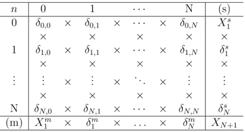
3.1 Information Structure of the MMFE . . . 45
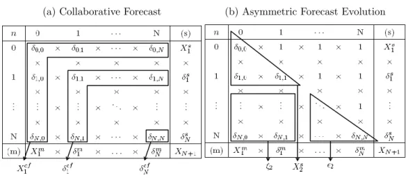
3.2 Information Structure of the multiplicative MMFE . . . 47
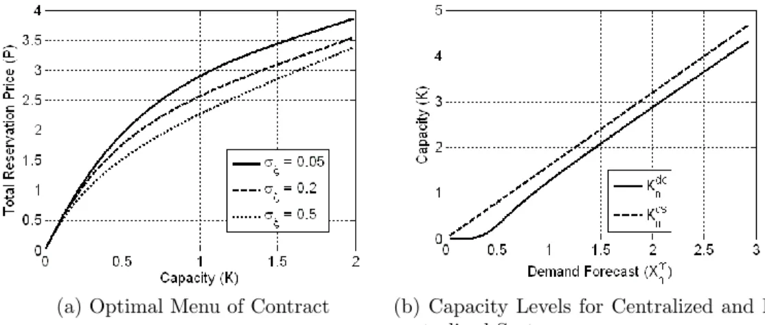
3.3 Optimal Capacity Reservation Contract . . . 65
4.1 Expected Values of Market Potential . . . 95
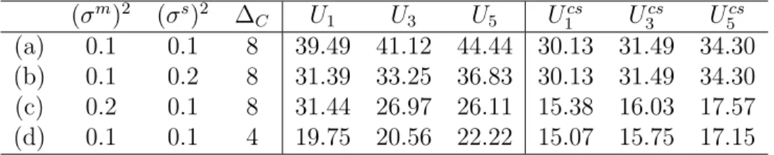
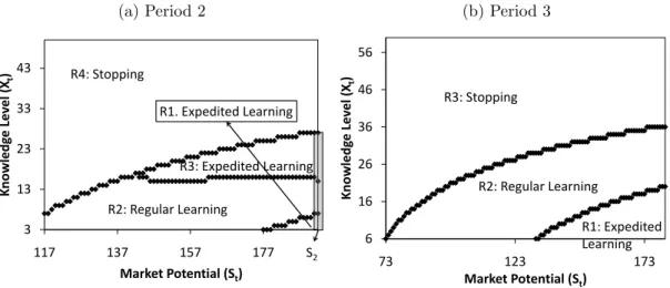
4.2 Optimal Investment and Stopping Policy of Base Numerical Setting . 96 4.3 Knowledge-Level-Based Upper Threshold Policy . . . 97
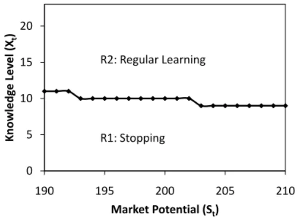
4.4 Market-Potential-Based Lower Threshold Policy . . . 98
4.5 Probability of Stopping at Period 3 . . . 99
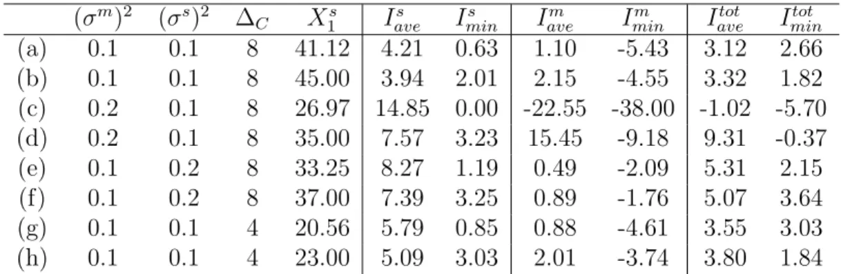
4.6 Impact of Uncertainties in Learning . . . 102
4.7 Impact of Reducible Unit Production Cost . . . 102
4.8 Impact of the Cost of Expedited Learning . . . 103
4.9 Impact of Uncertainties in Market Potential Change . . . 104
4.10 Impact of Demand Uncertainty . . . 105
4.11 Impact of the Size of the Salvage Market . . . 106
B.1 Information Structure of the additive MMFE . . . 118
Introduction
Optimal stopping problems determine the time to stop a process in order to maximize expected rewards. Such problems appear frequently in the areas of economics, finance, statistics, marketing and operations management. For example, a stock option holder faces the problem of determining the time to exercise the option in order to maximize the expected income. As another example, employers face the problem of determining the time to stop interviewing job candidates in order to hire the best candidate. This dissertation studies two important optimal stopping problems arising in Operations Management. It also provides a method that characterizes the structure of the optimal stopping policy for a general class of optimal stopping problems.
Optimal stopping problems often have simple threshold or control-band type op-timal stopping policies. For example, for an American put option, a threshold policy under which the option holder exercises the stock option if the current stock price is below a certain threshold is optimal. Such structural properties of the optimal stopping policy are important for three reasons. First, knowing the structure of the optimal policy provides managerial insights. They provide actionable policies that a decision maker can follow to optimize her objective. Second, structural results also enable one to develop efficient numerical algorithms to solve optimal stopping prob-lems. Finally, structural results are important when the optimal stopping problem is part of a higher-level and/or larger scale optimization problem. For these reasons,
most research papers that study optimal stopping problems provide structural prop-erties of the optimal stopping policy if such structures exist (see, e.g., Chen 1970, Yao and Zheng 1999b, Ben-Ameur et al. 2002, Alagoz et al. 2004).
In Chapter 2, we provide a method that characterizes the structure of the optimal stopping policy for the class of discrete-time optimal stopping problems. Our method is based on structural properties of the benefit function, which we define as the dif-ference between the reward of continuing the process and the reward of stopping the process. To characterize its structure, we establish the benefit function’s recursive relation with the one-step benefit function, which we define as the difference between the rewards of stopping at the next period and the current period. Using this recur-sive relation and the stochastic monotonicity of state-transition, we determine several sufficient conditions that yield threshold or control-band type optimal stopping poli-cies. We show that our method can characterize the structure of the optimal policy of some stopping problems for which conventional methods fail. We also show that the method simplifies the analysis of some existing results.
Next, in Chapter 3, we study an optimal stopping problem faced by a supplier who invests in new capacity. For a timely delivery, the supplier has to secure component capacity prior to receiving a firm order from a product manufacturer. The supplier relies on the demand forecast for his capacity decision. However, the manufacturer often has other forward-looking information because of her superior relationship with or proximity to the market and expert opinion about her own product. To elicit the manufacturer’s private information, the supplier needs to design and offer a screening contract. As the sales season approaches, both the supplier and the manufacturer can update their demand forecasts over time. Hence, by delaying to offer the screening contract, the supplier can reduce the demand uncertainty that he faces. However, delaying the capacity decision is not always beneficial for the supplier. For example, the delay may increase the degree of information asymmetry between the two firms if the manufacturer obtains more information than the supplier over time. Capacity costs may also increase as the supplier delays the capacity decision because of a tighter deadline for building capacity. By considering all such trade-offs, the supplier needs to determine when to offer a screening contract and how to design the screening contract
to maximize his profit. In Chapter 3, we develop an optimal stopping problem to solve this problem.
The supplier’s decision problem consists of two stages. The first stage is an optimal stopping problem that determines the optimal time to offer a screening contract, and the second stage is a mechanism design problem for forecast information sharing. Using the method that we develop in Chapter 2, we establish the optimality of a control band policy that prescribes when to offer an optimal incentive mechanism. Under this policy, the supplier offers a menu of contracts if the supplier’s demand forecast falls within the control band. We also provide structural properties of the optimal screening contract and explicitly show how the optimal contract depends on the demand forecast and how the timing decision affects the mechanism design problem. Through numerical studies, we characterize the environment in which the supplier should offer the contract late or early. By comparing the profits of the dynamic strategy with those of a static one in which the supplier offers a contract in a fixed period, we show that the supplier can significantly improve his profit by optimally determining the time to offer a contract. However, the results also show that this dynamic strategy can reduce the total supply chain efficiency.
Modeling the aforementioned stopping problem requires a forecast evolution model that describes forecast sequences made by two decision makers. To develop such a model, we extend the Martingale Model of Forecast Evolution (MMFE) framework to the cases with multiple decision makers in Chapter 3. The MMFE is a general model that describes the evolution of forecasts arising from many statistical and judgment-based forecasting methods. Due to its descriptive power and generality, researchers have used the MMFE in many studies that involve dynamic forecast updates such as inventory control and production planning (e.g., Heath and Jackson 1994, Aviv 2001, Gallego and ¨Ozer 2001, Toktay and Wein 2001, Altug and Muharremoglu 2009, Iida and Zipkin 2009, Schoenmeyr and Graves 2009). Our extension enables the MMFE framework to model several plausible forecast evolution scenarios that involve multiple decision makers in a consistent way.
Finally, in Chapter 4, we study an optimal stopping problem faced by a manufac-turer who introduces a new product to the market. When determining the timing for
introducing the new product, the manufacturer takes into consideration the trade-off between the time-to-market and the completeness of the production processes. On the one hand, the manufacturer can attain a large market share by entering the mar-ket early. On the other hand, the manufacturer can improve the production process for the new product by investing more time in process design, which results in a reduction of production costs. However, the manufacturer are uncertain about both the timing of the competitors’ market entry and the outcome of production process development activities. For this reason, the manufacturer needs to dynamically make the timing decision depending on the competitors’ movements and the readiness of his own production process. We formulate the manufacturer’s problem as an optimal stopping problem.
The manufacturer’s decision process also consists of two stages. The first stage is an optimal stopping problem that determines the optimal time to introduce a new product to the market and optimal investment decisions to improve the production process. The second stage is a production and pricing decision problem that deter-mines the production quantity and the sales prices for the new product. Using the method that we develop in Chapter 2, we establish the optimality of threshold-type market entry policies that prescribe the optimal time to introduce the new prod-uct. We also characterize structural properties of the optimal production and pricing decisions. By comparing to a static market entry decision, we show that the dy-namic market entry decision yields a higher and less variable profit. Our study also characterizes when the value of the dynamic market entry is the greatest.
Characterizing the Structure of the
Optimal Stopping Policy
2.1.
Introduction
Optimal stopping problems are determining the time to terminate a process to max-imize expected rewards given the initial state of the process. Such problems appear frequently in the operations, marketing, finance and economics literature. Some ex-amples are the problem of determining the time to exercise a stock option, to sell or purchase an asset, and to introduce a new product. Optimal stopping problems are rarely solvable in a closed form and they require computational methods. Hence, researchers often try to characterize the structure of the optimal stopping policy that determines when to stop the process based on the state of the process at each decision epoch. When possible, researchers also provide monotonicity results (comparative statics) regarding the optimal policy parameters. Such structural results enable ac-tionable policies that a decision maker can follow to maximize rewards. They also help develop efficient numerical algorithms to solve the problem. This chapter pro-vides a method to characterize the structure of an optimal stopping policy for the class of discrete-time optimal stopping problems. This chapter also determines suf-ficient conditions that yield simple threshold or control-band type stopping policies. These conditions are presented in eight propositions that can be used to characterize
optimal stopping policy for various application areas.
Structural properties of the optimal stopping policy are helpful for three reasons. First, knowing the structure of the optimal policy provides managerial insights. They provide actionable policies that a decision maker can follow to optimize her objective. For example, exercising an American put option (stopping the process) is optimal when the current stock price (current state) is below a certain threshold. Another ex-ample is from Alag¨oz et al. (2007a,b) who establish an optimal organ-transplantation policy for a patient with end-stage liver disease. They show that given the current health condition of the patient, transplanting an organ is optimal if the quality1 of the offered organ is above a certain level. Second, structural results also enable one to develop efficient numerical algorithms to solve optimal stopping problems (as in Yao and Zheng 1999b, Ben-Ameur et al. 2002, Wu and Fu 2003). For example, Wu and Fu (2003) first establish the optimality of a threshold-type exercise policy for an American-Asian option. Using this structure, they develop a computationally efficient simulation-based algorithm. Finally, structural results are important when the optimal stopping problem is part of a higher-level and/or larger scale optimiza-tion problem (Terwiesch and Xu 2004, Anily and Grosfeld-Nir 2006). For example, Terwiesch and Xu (2004) study a manufacturer’s problem of pricing prototypes and the final product. To do so, they first model a customer’s purchasing decision as an optimal stopping problem. They show that the customer’s optimal purchase policy has a threshold structure. Using this result, the authors formulate the manufac-turer’s optimal pricing problem. For aforementioned reasons, several other papers also characterize structural properties of optimal stopping policies for various stop-ping problems (such as Chow et al. 1964, Cox et al. 1979, Chen et al. 1998, and Boyaci and ¨Ozer 2009).
The above observations motivated us to identify a universal method that can help determine the structure of optimal stopping policy for problems arising in various fields. The method also helps us to identify sufficient conditions that yield simple optimal policies. Before discussing our new method, we describe the two approaches currently used in the literature. The first approach is to verify whether the problem
satisfies the monotone-case condition (Chow et al. 1971). This approach first deter-mines the set of states at which the reward of immediate stopping is greater than the expected reward of stopping at the next period. The policy that stops the process if the current state is in this set is known as the one-step look-ahead policy. Chow et al. (1971) show that if this set is closed almost surely2, then the one-step
look-ahead policy is optimal and call such a case the monotone-case. Since the one-step look-ahead policy is easy to compute and implement, researchers often try to verify whether the problem satisfies the monotone-case condition (see, for example, Stadje 1991, Hui et al. 2008). However, most optimal stopping problems do not satisfy the monotone-case condition because the one-step look-ahead policy, a myopic policy, is not optimal in general. The second and the most common approach is based on the dynamic programming formulation of the optimal stopping problem. This approach determines structural properties of the value function of the dynamic program to characterize the optimal stopping policy (see, for example, Wu and Fu 2003, Babich and Sobel 2004, and Alagoz et al. 2007a). As we will illustrate in §2.3, these two ap-proaches, although helpful, do not always yield the structure of the optimal stopping policy.
This chapter provides a different approach to characterize the structure of the optimal stopping policy. Our method is based on structural properties of the bene-fit function, which we define as the difference between the reward of continuing the process and the reward of stopping the process. To characterize its structure, we establish the benefit function’s recursive relation with the one-step benefit function, which we define as the difference between the rewards of stopping at the next pe-riod and the current pepe-riod. Next, we determine sufficient conditions that yield a threshold or control-band type optimal stopping policy using this recursive relation and the stochastic monotonicity of state-transition. We show that our method can characterize the structure of the optimal policy of some optimal stopping problems for which the two approaches discussed above fail to do so. We also show that the
2That is, when the current state is in this set, the future states will be in this set with probability
method simplifies the analysis of existing results. One can use the method to char-acterize the structure of the optimal policy before numerically solving the optimal stopping problem. The results also make the sufficient conditions that yield simple optimal stopping policies transparent and easier to determine.
For the analysis of our method, we use stochastic monotonicities of parameter-ized random variables. Stochastic monotonicities are widely used in the analysis of stochastic objective functions (Shaked and Shanthikumar 2007). For example, Athey (2000) uses them to characterize the structure of the objective functions that arise in economics. Smith and McCardle (2002) use them to characterize the structure of the value function of a Markov decision process (MDP). Even though optimal stop-ping problems are a sub-class of general MDPs, our method is not related to those in Smith and McCardle (2002). Our method for characterizing the structure of the optimal policy is based on the benefit function. The benefit function is the difference between the two reward functions: the expected reward of continuing the process and the reward of stopping the process. In contrast, the value function is the maximum of the two. Hence, the benefit function is different from the value function of MDPs. We show that the properties of the benefit function directly imply the structure of the optimal stopping policy when the structure of the value function and the result of Smith and McCardle (2002) do not. In addition, the benefit function and the value function have different recursions as we discuss in §2.2. Our approach is ef-fective because there are only two actions for optimal stopping problems. Despite its effectiveness and simplicity, this method has been neglected (see §2.3.2 for some examples). Our research formalizes this method in a general framework.
There has also been extensive research on the monotonicity of optimal control. Several researchers have provided sufficient conditions that yield monotone optimal policies (Altman and Stidham 1995 and Glasserman and Yao 1994). However, the monotonicity of the optimal policies in this stream of research is based on the theory of ordered optimal solutions by Topkis (1978) and its generalizations. For example, Altman and Stidham (1995) show that a threshold policy is optimal for stationary Markov decision processes with two actions when the reward function is submodular in state and action and the state transition is stochastically monotone. We remark that
none of the discrete-time optimal stopping problems satisfies Altman and Stidham (1995)’s assumptions set forth for binary Markov decision problems. Our method and sufficient conditions are based on the zero-crossing points of the benefit function and do not require the submodularity of reward functions. Hence, the results of this chapter can be applied to the problems that do not satisfy the sufficient conditions provided by the literature on monotone optimal control. We refer to Glasserman and Yao (1994) for additional references on this literature.
Due to the importance of stopping problems, extensive research has been done (Chow et al. 1971, Shiryaev 1978, Tsitsiklis and Van Roy 1999, Peskir and Shiryaev 2006). This line of research characterizes optimal stopping times and optimal re-wards under various general assumptions. However, this literature has not focused on characterizing the structure of the optimal stopping policy. Our study, in contrast, focuses on a method to characterize the structure of optimal stopping policies and determines sufficient conditions to obtain them.
The rest of this chapter is organized as follows. In §2.2, we define the optimal stopping problem and propose the method to characterize the structure of the op-timal stopping policy. In §2.3, we provide an example for which only our method can characterize the structure of the optimal policy and another example for which our method simplifies the analysis of an existing result. In §2.4, we provide sufficient conditions that yield a threshold or control-band type optimal stopping policy and provide monotonicity results and bounds for the optimal policy. In §2.5, we consider optimal stopping problems with additional decisions other than the stopping deci-sion. In §2.6, we consider infinite-horizon optimal stopping problems. In §2.7, we provide example applications to facilitate the use of the proposed method. In §2.8, we conclude. The objective of this chapter is to introduce an easy and useful method to researchers in broad application areas. Hence, in Appendix A.1, we provide a theorem and examples that one can use to verify stochastic monotonicities of state transition models. Proofs not provided right after the propositions are deferred to Appendix A.2.
2.2.
Optimal Stopping Problem and the Two-Step
Method
Let {xt|t = 1,2, . . . , T} be a Markov process that evolves in a state space X ⊂ Rd, defined on a probability space (Ω,F,P). We denote the σ-algebra generated by
{x1, x2, . . . , xt}byFt⊂ F. A stopping time τ is a random variable that takes values in{1,2, . . . , T} and satisfies {ω∈Ω|τ(ω)≤t} ∈ Ft for all t≤ T. We denote the set of all such stopping times by UT.
At each periodt∈ {1,2, . . . , T}, a decision maker observes the statextand decides whether to continue or stop a process. If the decision maker decides to continue, she attains a reward Ct(xt) and the state evolves. If she stops, then the decision maker attains a rewardSt(xt), and the problem is terminated. Without loss of generality, we assume that stopping is a forced decision at period T.3 In addition, we assume that reward functions Ct : Rd → R and St : Rd → R are integrable, i.e., E|St(xt)| < ∞ and E|Ct(xt)|<∞ for every t <∞. The objective is to determine the optimal time to stop the process in order to maximize the total discounted rewards with a discount factor α∈(0,1]. This problem can be formulated as
V∗(x)≡ sup τ∈UT E "τ−1 X t=1 αt−1Ct(xt) +ατ−1Sτ(xτ) x1 =x # . (2.1)
The optimal value function V∗(x) corresponds to the total expected reward when the optimal stopping time achieves the supremum in (2.1), and the initial state is
x. Note that the optimal stopping time and the optimal value function are well-defined. However, this formulation does not help characterize an actionable policy that a decision maker can follow to maximize her expected reward. Hence, we provide a dynamic programming (DP) recursion that specifies an optimal action for each state at each period.
3In some problems, not stopping and receiving a reward of 0 at the end of the decision horizon is
an option for the decision maker. For such problems, one can introduce a fictitious periodt=T+ 1 withST+1(xT+1) = 0, and enforce the stopping at periodt=T+ 1. Therefore, the forced stopping
Let UT
t be the set of stopping times that satisfy τ ∈[t, T]. Then, we define
Vt(x)≡ sup τ∈UT t E "τ−1 X u=t αu−tCu(xu) +ατ−tSτ(xτ) xt =x # ,
which indicates the total expected rewards from period t when the process has not yet stopped and the current state is x. If the decision maker stops the pro-cess at period t, the reward is St(x). If she continues, the expected reward is
Ct(x) +αE[Vt+1(xt+1)|xt = x]. Therefore, Vt(x) satisfies the following DP recursion (Theorem 3.2 of Chow et al. 1971):
Vt(xt) = max{St(xt), Ct(xt) +αE[Vt+1(˜xt+1(xt))]}, t < T, (2.2)
where VT(xT) =ST(xT). We denote E[Vt+1(xt+1)|xt] by E[Vt+1(˜xt+1(xt))] to empha-size its functional dependence on xt. Note that Vt(x) is the value function of the DP recursion, and the optimalvalue function satisfies V∗(x) =V1(x). An optimal policy
stops the process at period t if St(xt)≥Ct(xt) +αE[Vt+1(˜xt+1(xt))].
To date, the most common approach for characterizing the structure of the optimal stopping policy is based on characterizing structural properties of the corresponding value function. However, this approach is not always useful in characterizing the structure of the optimal stopping policy. Note that the optimal stopping decision is based on the relative values of St(xt) and Ct(xt) +αE[Vt+1(˜xt+1(xt))]. For example, the information thatVt+1(xt+1) is increasing inxt+1 is not useful in characterizing the
structure of the optimal policy, when bothSt(xt) and Ct(xt) +αE[Vt+1(˜xt+1(xt))] are increasing inxt. In contrast, the structural properties of
Bt(xt)≡αE[Vt+1(˜xt+1(xt))] +Ct(xt)−St(xt)
help directly characterize the optimal stopping policy because the optimal policy at each periodt < T is to stop the process ifBt(xt)≤0 and to continue, otherwise. We refer to this function as thebenefit function. It is the expected benefit of delaying the stopping decision at period t. For optimal stopping problems, determining structural
properties of the benefit function provides an easier way to characterize the optimal policy than determining structural properties of thevalue function. This approach is possible because optimal stopping problems have only two options to choose at each period: stop or continue.
We also define the one-step look-ahead, or in short, the one-step benefit function
Mt(xt)≡αE[St+1(˜xt+1(xt))] +Ct(xt)−St(xt),
which indicates the expected benefit of delaying the stopping decision at period t
without considering the possible benefit of delaying the decision beyond period t+ 1. These two functions are closely related. The following recursion formalizes this relationship: Bt(xt) = αE[Vt+1(˜xt+1(xt))] +Ct(xt)−St(xt) = αE[max{St+1(˜xt+1(xt)), Bt+1(˜xt+1(xt)) +St+1(˜xt+1(xt))}] +Ct(xt)−St(xt) = Mt(xt) +αE[max{0, Bt+1(˜xt+1(xt))}], t < T −1, (2.3) BT−1(xT−1) = MT−1(xT−1).
This recursive relationship highlights two important observations. First, struc-tural properties of the benefit function is closely related to that of the one-step ben-efit function. Second, these properties also depend on the functional form of the state transition ˜xt+1(xt) and the corresponding transition probabilities. Naturally, establishing structural properties of Bt(xt) from this recursive relationship involves an inductive argument. Suppose Mt(xt) has a certain structural property for every
t. Then BT−1(xT−1) inherits its structural property by definition. We will show that
when the state transition ˜xt+1(xt) has an appropriate stochastic monotonicity,Bt(xt) also has the same property with Mt(xt) for all other periods. The two-step method is based on this idea. In particular,
and x˜t+1(xt). Next, we verify whether x˜t+1(xt) has the stochastic
mono-tonicity that enables Bt(xt) to inherit the structural property of Mt(xt).
Then, structural properties ofBt(xt) directly imply the structure of the optimal stop-ping policy. For example, whenMt(xt) is increasing4 inxt, a stochastically increasing state transition ˜xt+1(xt) carries the increasing property toBt(xt). Hence, a threshold policy is optimal. We provide such sufficient conditions in§2.4, which corresponds to the second step. We provide several examples to illustrate the first step in §2.7.
2.3.
Two Example Applications
We introduce two examples that support the importance of our method discussed in the previous section. The first example illustrates that the conventional value-function-based approach for characterizing the structure of the optimal stopping pol-icy does not always work. This example also does not satisfy the monotone-case condition. Hence, the conventional methods discussed previously fail to characterize the optimal policy for this first example. However, the proposed method successfully characterizes the structure of the optimal policy. The second example illustrates how the two-step method substantially simplifies the analysis of an existing result.
2.3.1
Time-to-Market Model
Consider a firm that decides when to introduce a new product. When the firm introduces the product earlier than competitors, it captures a larger market share. However, an early introduction results in high production costs and low profit margins due to low manufacturing yields. Hence, the firm needs to determine the optimal time to enter the market. Suppose that the total market demandD is deterministic. There areT periods in which the firm can introduce the new product. At each period
t ∈ {1,2, . . . , T}, the firm decides whether to delay the market entry depending on the number of competitors who are already in the market, xt ∈ {0,1, . . .}. Let v(xt)
4We use the terms increasing and decreasing in the weak sense; i.e., increasing means
be the market share of the firm when she enters the market after thextth competitor. It is decreasing concave inxt. That is, as more competitors enter the market the firm loses more market share. Let p be the sales price of the product and ct be the unit production cost when the firm enters the market at period t. The discounted profit marginαt−1(p−c
t) increases witht due to higher manufacturing yields5. If the firm enters the market at period t, she attains a reward of St(xt) =v(xt)(p−ct)D. If she delays the market entrance at period t, then ξt more competitors enter the market, and the state evolves as ˜xt+1(xt) =xt+ξt. The random variable ξt is independent of
xt.
This problem can be formulated as an optimal stopping problem. The value function is derived asVt(x) = supτ∈UT
t E ατ−1S τ(xτ) xt =x
and the benefit function is derived as Bt(xt) = αE[Vt+1(˜xt+1(xt))]−St(xt). The DP recursion is given by
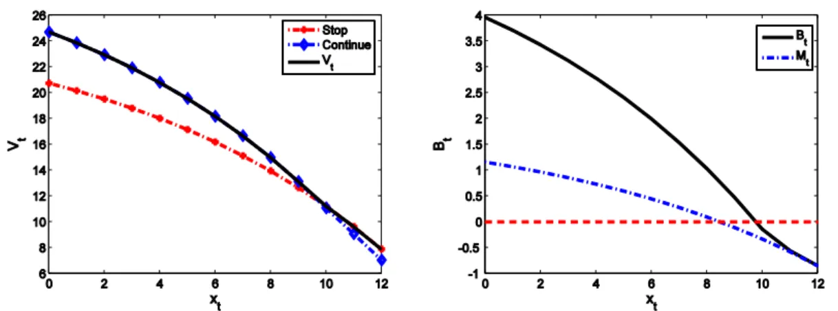
Vt(xt) = max{St(xt), αE[Vt+1(˜xt+1(xt))]} with VT(xT) = ST(xT). Figure 2.1 shows an example of Vt(xt), Bt(xt), and Mt(xt) for t = 13. The problem setting for this example is T = 15, α= 1, v(x) = 0.9−0.85e0.1(x−15), p= 5, ct = 4−0.1t−0.005t2,
D= 10, and ξt is a Bernoulli r.v. with 0.7.
Figure 2.1: Value function and the benefit function of the time-to-market problem
First note from Figure 2.1 that Mt(x) and Bt(x) do not cross the zero line at the same point. The monotone-case condition of Chow et al. (1971) is also not satisfied.
5This example is a simplified version of a problem faced by Hitachi GST, a global provider of
Hence, the one-step look ahead policy is not optimal. Second, note that although the reward functionSt(xt) is decreasing concave in xt for every t, the value function
Vt(xt) is not concave in xt. The decreasing property of Vt(xt) in xt does not provide any information about the optimal stopping policy, either. The value function is the maximum of the reward of stopping and the reward of continuing, which are both decreasing in xt. Hence, structural properties of the value function (and hence the methods of Smith and McCardle 2002) cannot characterize the structure of the optimal stopping policy in this case. However, by using the two-step method, we can easily verify the decreasing property of Bt(xt), which establishes the optimality of a threshold policy; i.e., the firm should enter the market at period t if xt ≥ xt for a certain threshold xt. We provide the complete analysis in §2.7.
2.3.2
American-Asian Option
Our second example is the problem of pricing an American-Asian option studied in Ben-Ameur et al. (2002) and Wu and Fu (2003). A stock option is a financial derivative security that promises the option holder a payoff when the holder exercises the option. The payoff depends on the future prices of an underlying stock and the agreed upon strike price K. A holder of the American-Asian option can exercise the stock option at fixed periods t ∈ {1,2, . . . , T + 1}.6 The payoff depends on the average price of the underlying stock, where the average is taken for the stock prices at periods 1,2, . . . , t. Letxt,1be the current stock price at periodtandxt,2be the average
stock price at period t. If the option holder exercises the option at period t≤T, she receives a rewardSt(xt) =xt,2−K. If the option holder does not exercise the option at
periodt, the stock price changes as ˜xt+1,1(xt) = ξxt,1, whereξ is a log-normal random
variable. Accordingly, the average stock price is updated as ˜xt+1,2(xt) =
txt,2+ξxt,1 t+1 . If
the option is not exercised in any periods, thenST+1(·) = 0. By using the risk-neutral
measure (Black and Scholes 1973, Harrison and Kreps 1979) of ξ, the option pricing problem can be formulated as an optimal stopping problem. The price of the option is the optimal value function of the stopping problem, and the optimal exercise policy
6PeriodT + 1 is a fictitious period, which gives the option holder the right not to exercise the
is the optimal stopping policy. The discount factor isα=e−r, whereris the risk-free interest rate. The value function is derived asVt(x) = supτ∈UT
t E ατ−tSτ(xτ) xt=x
and the benefit function is derived as Bt(xt) =αE[Vt+1(˜xt+1(xt))]−St(xt). The DP recursion is given by Vt(xt) = max{St(xt), αE[Vt+1(˜xt+1(xt))]} with VT+1(xT+1) = 0.
Ben-Ameur et al. (2002) and Wu and Fu (2003) independently determine the struc-ture of the optimal policy based on the properties of thevaluefunction. For example, Proposition 1 (in Ben-Ameur et al. 2002) verifies that St(xt) and αE[Vt+1(˜xt+1(xt))] are increasing and convex inxt,1 andxt,2. However, this information does not
charac-terize the structure of the optimal policy. Instead, both of these papers establish the optimality of a state-dependent threshold policy by verifying that the increasing rate of αE[Vt+1(˜xt+1(xt))] inxt,2 is less than or equal to 1. Although elegant, establishing
the structure of the optimal policy using the value function requires a lengthy anal-ysis that involves three propositions and one lemma (§4 in Ben-Ameur et al. 2002). However, as we will show in §2.7, the two-step method can be used to easily verify that the benefit functionBt(xt) is decreasing in xt,2. This result directly implies the
optimality of astate-dependentthreshold policy. Under this policy, the option holder optimally exercises the option at period t if xt,2 ≥ xt,2(xt,1) for certain thresholds
xt,2(xt,1). We provide the complete analysis in §2.7.
2.4.
Conditions that Imply the Structure of the
Optimal Policy
We provide sufficient conditions onMt(xt) and ˜xt+1(xt) that together imply the struc-ture of the benefit function Bt(xt) and the optimal stopping policy. We also establish some monotonicity results and bounds for the optimal policy parameters. The result of this section corresponds to the second step of the two-step method.7
7We remark that the results of this section are not related to those in in Chow et al. (1971) and
they do not imply the optimality of the one-step look-ahead policy. This policy calls for stopping the process when the reward of instant stopping is greater than the expected reward of stopping at the next period, i.e., whenMt(xt)≤0. The one-step look-ahead policy is generally sub-optimal. Chow
et al. (1971) provide sufficient conditions under which the one-step look-ahead policy is optimal and refer to it as the monotone-case. In the monotone-case, {x: Mt(x)≤0} ={x: Bt(x) ≤0}. The
For the case of a multi-dimensional state space, we denote the ith element of the vector xt by xt,i and thed−1 dimensional vector excluding the element xt,i from xt by xt,−i. Similarly, xt,−(i,j) denotes the d−2 dimensional vector excluding elements
xt,i and xt,j fromxt. We write (x
0
t,i, xt,−i) for the state (xt,1, xt,2, . . . , x
0
t,i, . . . , xt,d) and write (x0t,i, x00t,j, xt,−(i,j)) for the state (xt,1, xt,2, . . . , x
0
t,i, . . . , x
00
t,j, . . . , xt,d).
We also define the stopping set of period t as {x ∈ X : Bt(x) ≤ 0}. It is the set of states for which the optimal policy stops the process at period t. For a single-dimensional state space problem, we define xt ≡ sup{x ∈ X : Bt(x) ≤ 0} and
xt≡inf{x∈X :Bt(x)≤0}. Similarly, for a multi-dimensional state space problem, we define xt,i(xt,−i) ≡sup{xt,i : Bt(xt,i, xt,−i) ≤0, xt ∈X} and xt,i(xt,−i) ≡inf{xt,i :
Bt(xt,i, xt,−i)≤0, xt∈X}.
2.4.1
Univariate Benefit Functions
Consider optimal stopping problems with a single-dimensional state space and an increasing or decreasing one-step benefit function. Before stating the first proposi-tion, we define the stochastic monotonicity necessary for the analysis. We follow the definitions in Shaked and Shanthikumar (2007) for all stochastic monotonicities.
Definition 2.1. A set of random variables {x˜(θ), θ ∈R} is stochastically increasing in θ if E[u(˜x(θ))]is increasing in θ for all increasing functions u.
We note that many common Markov process models have this property. In Ap-pendix A.1, we provide a theorem and examples that one can use to verify stochastic monotonicities of state transitions. Using this definition, we provide the first sufficient condition.
Proposition 2.1. When Mt(xt) is increasing [resp., decreasing] in xt, and x˜t+1(xt)
is stochastically increasing in xt for every t, then the following statements are true
for every t:
1. Bt(xt) is increasing [resp., decreasing] in xt.
2. A threshold policy that stops the process if xt≤xt [resp., xt≥xt] is optimal.
Proof. The proof is based on an induction argument. Consider the increasing one-step benefit function case. At period t = T − 1, we have BT−1(x) = MT−1(x).
Hence, Bt(x) is increasing in x for t = T − 1. Next assume for the induction argument that Bt+1(xt+1) is increasing in xt+1. The composition of an increasing
function and max{0, x} is also increasing, hence, max{0, Bt+1(x)} is an increasing
function. Because the state transition ˜xt+1(xt) is stochastically increasing in xt,
E[max{0, Bt+1(˜xt+1(xt))}] is increasing in xt. Because the increasing property is closed under summation, Bt(xt) = Mt(xt) +αE[max{0, Bt+1(˜xt+1(xt))}] is increas-ing in xt, which concludes the induction hypothesis and the proof of Part 1 for the increasing Mt(x) case.
To prove Part 2, we define two sets Q = {x ∈ X : x ≤ xt} and Q∗ = {x ∈
X : Bt(x) ≤ 0}. We prove that Q = Q∗. When the state space is discrete or
Bt(xt) is a continuous function, xt satisfies Bt(xt) = 0. Then, every x ∈ Q satisfies
Bt(x) ≤ Bt(xt) = 0 because Bt(xt) is increasing. Hence, Q ⊂ Q∗. Conversely, for every x ∈Q∗, we have x≤xt by the definition of xt. Hence,Q∗ ⊂Q, which implies that Q = Q∗. Therefore, the optimal stopping policy stops the process at period t
if xt ∈ Q, i.e., if xt ≤ xt. Note that when the state space is continuous and Bt(xt) has a discontinuous point, it is possible that Bt(xt) > 0. In this case, the optimal policy stops the process if xt< xt instead of xt ≤xt. However, the structural result does not change. Hence, we assume throughout this chapter thatBt(xt) is continuous when the state space is continuous. The decreasing case can be proved in a similar way.
Recall that the recursive relationship in Equation (2.3) has max{0,·}. In general, max{0, f(x)} does not preserve structural properties off(x). Increasing, decreasing and convex properties are among the few properties that are preserved under this operation. Even concavity is not preserved. Other properties, such as subadditivity inxtare preserved, but those properties are not useful in characterizing the structure of the optimal stopping policy. Note that the structure of the optimal policy does not depend on the maximum point of Bt(xt), but depends on the pattern of Bt(xt)
crossing 0. Hence, we focus on increasing, decreasing, and convex properties.
Next, consider optimal stopping problems with a single-dimensional state space and a convex one-step benefit function. For the next result, we need a stochastically convex state transition.
Definition 2.2. A set of random variables {x˜(θ), θ ∈ R} is stochastically convex in
θ if E[u(˜x(θ))] is convex in θ for all convex functions u.
Using this definition, we provide the second sufficient condition.
Proposition 2.2. When Mt(xt)is convex in xt, and x˜t+1(xt)is stochastically convex
in xt for every t, then the following statements are true for every t:
1. Bt(xt) is convex in xt.
2. A control-band policy that stops the process if xt∈[xt, xt] is optimal.
2.4.2
Multivariate Benefit Functions with a Partially
Depen-dent State Transition
Consider optimal stopping problems with ad-dimensional state space. We consider a partially dependent state transition in which there exists an element i such that the state transition ˜xt+1,−i(xt) is independent ofxt,i. In other words, statext,i affectsonly theith element of the next period’s state. In this case, the state transition can be ex-pressed as ˜xt+1(xt) = (˜xt+1,i(xt),x˜t+1,−i(xt,−i)). Note that ˜xt+1,i(xt) can still depend on xt,−i in addition to depending xt,i. Note also that a special case of the partially dependent state transition is the fully independent state transition case, in which the state transition can be expressed as ˜xt+1(xt) = (˜xt+1,1(xt,1),x˜t+1,2(xt,2), . . . ,x˜t+1,d(xt,d)).
To better understand this case, recall the American-Asian option pricing problem discussed in§2.3.2. The state transition of the current stock price is ˜xt+1,1(xt) =ξxt,1.
This update is stochastically increasing inxt,1 but is independent ofxt,2. However, the
state transition of the average stock price ˜xt+1,2(xt) =
txt,2+ξxt,1
t+1 is stochastically
in-creasing in bothxt,1 andxt,2. Next, we provide sufficient conditions for the optimality
Proposition 2.3. When Mt(xt) is increasing [resp., decreasing] in xt,i, x˜t+1,i(xt) is
stochastically increasing in xt,i and x˜t+1,−i(xt) is independent of xt,i for every t, then
the following statements are true for every t: 1. Bt(xt) is increasing [resp., decreasing] in xt,i.
2. A state-dependent threshold policy that stops the process when xt,i ≤ xt,i(xt,−i)
[resp., xt,i ≥xt,i(xt,−i)] is optimal for each xt,−i.
Proposition 2.4. When Mt(xt) is convex in xt,i, x˜t+1,i(xt) is stochastically convex
in xt,i and x˜t+1,−i(xt)is independent of xt,i for every t, then the following statements
are true for every t:
1. Bt(xt) is convex in xt,i.
2. A state-dependent control-band policy that stops the process when
xt,i ∈[xt,i(xt,−i), xt,i(xt,−i)] is optimal for each xt,−i.
2.4.3
Multivariate Benefit Functions with a Dependent State
Transition
Elements of the state transition ˜xt+1(xt) are dependent on each other when the ith element of the next period state ˜xt+1,i(xt) depends on the ith element of the current state and also on the other elements of the current state. An interesting analysis can be applied to the case where the state transition ˜xt+1(xt) is stochastically increasing in xt. Note that the statext has multiple dimensions in this case. Hence, we need a more general definition of the stochastically increasing property.
Definition 2.3. A set of random vectors {x˜(θ), θ ∈Rd} of dimension m is
stochas-tically increasing in θ ∈ Rd if E[u(˜x(θ))] is increasing for all increasing functions
u:Rm →
R.
Given this definition, we have the following result.
Proposition 2.5. WhenMt(xt)is increasing[resp., decreasing] in eachxt,i andx˜t+1(xt)
is stochastically increasing in xt ∈ X for every t, then the following statements are
1. Bt(xt) is increasing [resp., decreasing] in each xt,i.
2. A state-dependent threshold policy that stops the process when xt,i ≤ xt,i(xt,−i)
[resp., xt,i ≥xt,i(xt,−i)] is optimal for each i.
At first sight, the conditions that the one-step benefit function is increasing in xt,i for all elements i and that the state transition is stochastic increasing appear to be somewhat restrictive. Consider, for example, a two-dimensional state space in which a higher value of xt,2 leads to a lower value of xt,1 in the next period. In this case,
one can redefine the state variable as yt,2 = −xt,1 and yt,1 = xt,1, which makes the
state transition ˜yt,1(yt) stochastically increasing in both yt,1 and yt,2. Similarly, if
an initial formulation of Mt(xt) is increasing in xt,1 and decreasing in xt,2, a similar
transformation makes the one-step benefit function Mt(yt) an increasing function. Therefore, the increasing benefit-function condition is not too restrictive. In general, one element of the current state may impact some elements of the next period state but not all of them. Suppose ˜xt+1,i(xt) is independent ofxt,j for somej 6=i. Then, by definition ˜xt+1,i(xt) is stochastically increasing in xt,j. Therefore, the stochastically increasing property of multi-dimensional state transition can also be satisfied easily.
Cases in which the state transition depends only on parts of the state space can be analyzed following the analyses given in this and the previous subsections. For example, consider the case in which the state transition of a three-dimensional state space ˜xt+1(xt) can be separated into ˜xt,(1,2)(xt,(1,2)) and ˜xt,3(xt,3), where the random
transition ˜xt,(1,2)(xt,(1,2)) is stochastically increasing in xt,(1,2). If the one-step benefit
functionMt(xt) is increasing in both xt,1 and xt,2, we can apply a slight modification
of Proposition 2.5 to xt,(1,2) for each fixed xt,3. We omit the proposition and the
analysis to avoid repetition.
2.4.4
Monotonicity Results and Bounds for Optimal
Thresh-olds
We discuss two types of monotonicity results for the optimal thresholds. The first one is the parametric monotonicity of the state-dependent optimal thresholds. The
second one is the time-monotonicity of optimal thresholds. We also provide bounds for the optimal thresholds. The result of this subsection is useful for developing efficient numerical algorithms. They also help characterize how policy parameters respond to the changes in the environment.
Proposition 2.6. The following statements are true for every t:
1. If Bt(xt) is increasing [resp., decreasing] in both xt,i and xt,j for i 6= j, then
xt,i(xt,−i)[resp., xt,i(xt,−i)] is decreasing in xt,j and xt,j(xt,−j)[resp., xt,j(xt,−j)]
is also decreasing in xt,i.
2. If Bt(xt) is increasing in xt,i and decreasing in xt,j for i 6=j, then xt,i(xt,−i) is
increasing in xt,j and xt,j(xt,−j) is also increasing in xt,i.
3. If Bt(xt) is increasing [resp., decreasing] in xt,i and convex in xt,j for i 6= j,
thenxt,j(xt,−j)is increasing [resp., decreasing] inxt,i andxt,j(xt,−j)is decreasing
[resp., increasing] in xt,i.
Next we consider time-monotonicity of optimal thresholds in stationary optimal stopping problems. An optimal stopping problem is stationary if the Markov process
xtis time-homogeneous and the reward functionsC(xt) and S(xt) are time-invariant. It is a well-known result that the value function Vt(x) is decreasing in t for every
x in such problems. See, for example, §4.4 of Bertsekas (2005). As t increases, the decision maker has less opportunity to delay the stopping decision, hence the value function Vt(x) decreases in t. This property directly implies that Bt(x) is decreasing int, which in turn implies the following proposition.
Proposition 2.7. For stationary optimal stopping problems, the following statements are true:
1. xt is increasing in t and xt is decreasing in t.
2. xt,i(xt,−i) is increasing in t and xt,i(xt,−i) is decreasing in t for every xt,−i. Finally, we provide bounds for the optimal thresholds. By definition, Bt(xt) ≥
period t with xt, i.e., Mt(xt) >0, then the optimal policy also continues the process at period t, i.e, Bt(xt)>0. This property implies the following proposition.
Proposition 2.8. The optimal thresholds have the following bounds: 1. xt≤sup{x∈X :Mt(x)≤0} and xt≥inf{x∈X :Mt(x)≤0}.
2. xt,i(xt,−i) ≤ sup{xt,i : Mt(xt,i, xt,−i) ≤ 0, xt ∈ X} and xt,i(xt,−i) ≥ inf{xt,i :
Mt(xt,i, xt,−i)≤0, xt ∈X}.
Note that determining the x that satisfies sup{x ∈ X : Mt(x) ≤ 0} is simple and does not involve recursive computation. Often it can be derived in a closed form. Hence, these bounds together with the monotonicity results considerably help reduce the computational time required to determine the optimal thresholds and resulting expected profit by reducing the search region. They also provide qualitative understanding of a decision process modeled as an optimal stopping problem.
2.5.
Optimal Stopping Problems with Additional
Decisions
The general theory of optimal stopping has focused primarily on problems in which stopping time is the only decision to make. Yet, it is possible to have optimal stopping problems with additional decisions. In particular, at each decision period
t∈ {1,2, . . . , T}, a decision maker observes the statext∈X of a process and decides whether to stop or continue the process. When stopping the process, the decision maker attains a reward of St(xt) and the process is terminated. When continuing the process, the decision maker takes an actionat ∈Atand attains a reward ofCt(at, xt). Then, the state evolves. The state transition depends on both xt and at, and we de-note it by ˜xt+1(at, xt). The action setAtis independent of the state. Letπbe a policy that specifies both the action to take for every t and every xt and the stopping time
τ that satisfy τ ≤T. Let ΠT be the set of all admissible policies. Then, the decision maker’s optimal stopping problem is to determine the optimal action to take and the
optimal time stop the process in order to maximize the total discounted rewards. We can formulate this problem as
V∗(x)≡ sup π∈ΠT E "τ−1 X t=1 αt−1Ct(at, xt) +ατ−1Sτ(xτ) x1 =x # .
The following DP specifies the optimal action for each state at each period.
Vt(xt) = max{St(xt), sup at∈At
[Ct(at, xt) +αE[Vt+1(˜xt+1(at, xt))]]}, t < T, (2.4)
where VT(xT) =ST(xT). The optimal value function satisfiesV∗(x) =V1(x). An
op-timal policy stops at periodt if St(xt)≥supat∈At[Ct(at, xt) +αE[Vt+1(˜xt+1(at, xt))]].
The optimal action when continuing the process at period t is the maximizer of the function inside sup[·]. Note that the optimal action depends on the state. Then, we define the one-step benefit function and the benefit function as
Mt(at, xt) ≡ αE[St+1(˜xt+1(at, xt))] +Ct(at, xt)−St(xt),
Bt(at, xt) ≡ αE[Vt+1(˜xt+1(at, xt))] +Ct(at, xt)−St(xt).
Additionally, we define the maximal benefit function as Bt(xt) ≡supat∈AtBt(at, xt).
We have: Bt(at, xt) = αE[Vt+1(˜xt+1(at, xt))] +Ct(at, xt)−St(xt) =αEmax0, Bt+1(˜xt+1(at, xt)) +St+1(˜xt+1(at, xt)) +Ct(at, xt)−St(xt) =Mt(at, xt) +αE max 0, Bt+1(˜xt+1(at, xt)) , t < T −1, (2.5) BT−1(aT−1, xT−1) =MT−1(aT−1, xT−1).
Note that the optimal policy stops the process at period t when Bt(xt)≤0. Hence, we need to determine structural properties of Bt(xt) to characterize the structure of the optimal stopping policy. However, even when Bt(at, xt) has a certain structural property in xt for each fixed at, Bt(xt) is not guaranteed to have the same property, because the optimal action depends on xt. Fortunately, increasing, decreasing and
convex properties are preserved under maximization. Following the two-step method, we provide the following sufficient conditions for the case of a single-dimensional state space. We define xt≡sup{x∈X :Bt(x)≤0} and xt≡inf{x∈X :Bt(x)≤0}. Proposition 2.9. WhenMt(at, xt)is increasing [resp., decreasing] inxt, andx˜t+1(at, xt)
is stochastically increasing inxt∈X for everyatand everyt, then the following
state-ments are true for every t:
1. Bt(xt) is increasing [resp., decreasing] in xt.
2. A threshold policy that stops the process if xt≤xt [resp., xt≥xt] is optimal.
Proof. We prove the first part; then the second part follows Proposition 2.1 Part 2. The proof is based on an induction argument. Consider the increasing one-step bene-fit function case. At periodt=T−1, we haveBT−1(at, x) = MT−1(at, x).Leta∗t(x) = arg maxat∈AtBt(at, x). For any x
1 ≤ x2, we have B
T−1(x1) = BT−1(a∗T−1(x1), x1) ≤
BT−1(a∗T−1(x1), x2) ≤ BT−1(a∗T−1(x2), x2), where the first inequality is from the fact
that BT−1(a, x) is increasing in x, and the second inequality is by the definition of
a∗T−1(x). Next assume for the induction argument that Bt+1(xt+1) is increasing in
xt+1. The composition of an increasing function and max{0, x} is also increasing,
hence, max{0, Bt+1(x)} is an increasing function of x. Because the state transition
˜
xt+1(at, xt) is stochastically increasing in xt, E[max{0, Bt+1(˜xt+1(at, xt))}] is increas-ing inxt for each at. Because the increasing property is preserved under summation, the benefit functionBt(at, xt) = Mt(at, xt)+αE[max{0, Bt+1(at,x˜t+1(xt))}] is increas-ing in xt for each at. By applying the same argument that we applied on BT−1(x),
we can verify thatBt(xt) = supat∈AtBt(at, xt) is increasing inxt, which concludes the
induction hypothesis and the proof of the proposition.
Proposition 2.10. When Mt(at, xt)is convex in xt, and x˜t+1(at, xt) is stochastically
convex in xt∈X for every at and every t, then the following statements are true for
every t:
1. Bt(xt) is convex in xt.
We can derive a similar result for the case of the multi-dimensional state space as in§2.4. We omit the discussion here to avoid repetition.
2.6.
Infinite-Horizon Optimal Stopping Problems
Here, we show that the results of this chapter can be applied to infinite-horizon optimal stopping problems. First, we define the infinite-horizon optimal stopping problem. As before,{xt|t= 1,2, . . .}is a Markov process that evolves in a state space
X ⊂ Rd. A stopping time τ is a random variable that takes values in {1,2, . . . ,∞} and satisfies {ω ∈ Ω|τ(ω) ≤ t} ∈ Ft for all finite t. We denote the set of all such stopping times by U. In the infinite-horizon case, we limit our interest to problems with a time-homogeneous Markov process and reward functions that are integrable. Unlike in the finite-horizon case, the stopping time can have an infinite value; hence, we need to agree onS(xτ) forτ =∞. Clearly, if limt→∞S(xt) exists, then it is natural to set S(xτ) to this value. Otherwise, we can set S(xτ) to be a fixed value, such as 0, or set S(xτ) = lim supt→∞S(xt), but this choice depends on the specific problem setup. Our results are valid regardless of this choice. As before, the decision maker’s optimal stopping problem is the problem of determining the optimal time to stop the process in order to maximize the total discounted rewards. We can formulate this problem as V∗(x)≡sup τ∈U E "τ−1 X t=1 αt−1C(xt) +ατ−1S(xτ) x1 =x # . (2.6)
Unlike in the finite-horizon case, a DP recursion is not possible because the backward recursion requires a well-defined final period. To apply the two-step method, we consider aT-period optimal stopping problem that has the same Markov process and the reward functions as the infinite-horizon problem. We use the notation (·|T) to emphasize that the functions we consider are the finite horizon counter parts of the infinite horizon problem. For example, we denote the optimal value function of the
T-period problem by V∗(x|T). Because the infinite-horizon problem can be seen as a finite-horizon problem with a long decision horizon, one can conjecture that the
optimal value function of the infinite horizon problem is the limit of the sequence of optimal value functions of finite-horizon problems, i.e.,V∗(x) = limT→∞V∗(x|T). In
many cases, the optimal value function also satisfies the Bellman equation V∗(x) = max{S(x), C(x) +αE[V∗(˜x(x))]}, where ˜x(x) denotes the one-step state transition, and a stationary policy that stops the process if S(x) ≥ C(x) +αE[V∗(˜x(x))] is optimal. Although these properties do not always hold, researchers have found several sufficient conditions that guarantee these properties. For example, optimal stopping problems with negative reward functions satisfy these properties as noted in §3.1 of Bertsekas (2007). Shiryaev (1978) also provides several such conditions. The two-step method can be applied to all infinite-horizon problems with these properties. Therefore, instead of providing a sufficient condition, we directly assume the following properties for all infinite-horizon problems we consider:
Assumption 2.1. 1. V∗(x) = max{S(x), C(x)+αE[V∗(˜x(x))]}, and a stationary policy that stops the process if S(x)≥C(x) +αE[V∗(˜x(x))] is optimal.
2. limT→∞V∗(x|T) = V∗(x).
As before, we define the one-step benefit function and the benefit function as
M(x)≡αE[S(˜x(x))] +C(x)−S(x) and B∗(x)≡αE[V∗(˜x(x))] +C(x)−S(x). From Part 1 of Assumption 2.1, a stationary policy that stops the process if B∗(x)≤ 0 is optimal. Then, the following proposition constructs the relationship between B∗(x) and B1(x|T) and the optimal thresholds. Before stating the proposition, we define
x ≡ sup{x ∈ X : B∗(x) ≤ 0} and x ≡ inf{x ∈ X : B∗(x) ≤ 0} for the case of a single-dimensional state space and define xi(x−i) ≡sup{xi :B∗(xi, x−i)≤ 0, x ∈X} and xi(x−i) ≡ inf{xi : B∗(xi, x−i) ≤ 0, x ∈ X} for the case of a multi-dimensional state space. Similarly, we denote the thresholds of the T-period problem byxt|T,xt|T,
xt,i|T(x−i) andxt,i|T(x−i).
Proposition 2.11. For infinite-horizon problems that satisfy Assumption 2.1, the following statements are true:
1. B1(x|T)↑B∗(x) as T → ∞.
Increasing, decreasing and convex properties are preserved under limit. Hence, when B1(x|T) has any of these structural properties for every T, B∗(x) also has the
same structural property. Therefore, we can apply the results of previous sections to infinite-horizon problems as follows: First, fix a finite time horizonT. Next, determine a structural property of B1(x|T) using the results of previous sections. Verify these
properties are preserved under limit. If so, the structure of the optimal policy follows from the finite horizon counter part. Consider, for example, the case in which the state space is single-dimensional, M(x) is increasing in x and ˜x(x) is stochastically increasing inx. Proposition 2.1 implies thatB1(x|T) is increasing inxfor every finite
T. Then, from Proposition 2.11, B∗(x) = limT→∞B1(x|T), which implies thatB∗(x)
is also increasing inx. WhenB∗(x) is increasing inx, it is optimal to stop the process if x ≤ x. Hence, a threshold policy that stops the process if x ≤ x is optimal. We can apply similar arguments to other cases.
Part 2 of Proposition 2.11 is useful when running the value iteration algorithm (Bertsekas 2005 Section 7) to solve the infinite horizon problem. The value iteration algorithm is based on Part 2 of Assumption 2.1. It recursively computes V∗(x|T) =
V1(x|T), which converges to V∗(x) as T → ∞.8 From the time-homogeneity of the
state transition and the reward functions, we have Vt(x|T) = Vt+1(x|T + 1), which
implies V1(x|T + 1) = max{S(x), C(x) +αE[V2(˜x(x)|T + 1)]} = max{S(x), C(x) +
αE[V1(˜x(x)|T)]}. Hence, the value iteration recursion is as follows:
V1(x|T + 1) = max{S(x), C(x) +αE[V1(˜x(x)|T)]}, (2.7)
where V1(x|1) = S(x). Then, consider the case in which B1(x|T) is increasing in x.
From the proposition, we have x1|T ≥ x1|T+1. By the definition of x1|T+1, we have
S(x)< C(x) +αE[V2(˜x(x)|T + 1)] for every x > x1|T+1. Because x1|T ≥x1|T+1 and
V2(x|T + 1) = V1(x|T), we have S(x) < C(x) +αE[V1(˜x(x)|T)] for every x > x1|T. Hence, we need not compute the value of S(x) in (2.7) for x > x1|T. One can apply similar arguments to the other cases.
8We do not need to computeB
1(x|T) to determine the optimal policy. The benefit function is
2.7.
Example Applications
We apply the two-step method to some optimal stopping problems from the literature including those discussed in §2.3. The objective of this section is three-fold: (1) We illustrate how to use the two-step method to obtain structural results. (2) We show that this method can be used for a variety of applications that arise in fields such as Finance, Marketing and Operations. Hence, the approach can be used for broad application areas. (3) We illustrate that the method makes it easy and transparent to characterize structural results. This transparency also allows one to obtain some results that were not reported in the original papers.
In what follows, we do not state all the assumptions, model elements and results from each paper but instead focus on the basic model and the optimal policy. For each example, we first show how to obtain structural properties of the one-step benefit function. Next, we characterize the structure of the optimal policy using the results of §2.4-2.6. We refer the reader to Appendix A.1 for the stochastic monotonicities of state transitions.
2.7.1
Time-to-Market Model
Recall the time-to-market model from §2.3.1. The reward function and the state transition of this problem have the following properties:
1. St(xt) = v(xt)(p−ct)D. 2. Ct(xt) = 0.
3. ˜xt+1(xt) =xt+ξt, whereξt≥0 is independent of xt. The one-step benefit function can be expressed as
Mt(xt) = αE[St+1(˜xt+1(xt))]−St(xt)
= αE[v(xt+ξt)−v(xt)](p−ct+1)D+v(xt)(α(p−ct+1)−p+ct)D. The first term is decreasing in xt because E[v(xt +ξt)−v(xt)] is decreasing in xt due to concavity of v(x). The second term is also decreasing in xt because v(xt) is