Keil_unc_0153D_14884.pdf

HEALTHY WORKER SURVIVOR BIAS IN A COHORT OF URANIUM MINERS FROM THE COLORADO PLATEAU

Alexander P Keil

A dissertation submitted to the faculty of the University of

North Carolina at Chapel Hill in partial fulfillment of the requirements for the degree of Doctor of Philosophy in the Department

of Epidemiology

Chapel Hill 2014

Approved by:

ABSTRACT

ALEXANDER KEIL: HEALTHY WORKER SURVIVOR BIAS IN A COHORT OF URANIUM MINERS FROM THE COLORADO PLATEAU

(Under the direction of David Richardson)

TABLE OF CONTENTS

LIST OF TABLES . . . x

LIST OF FIGURES. . . xii

LIST OF ABBREVIATIONS. . . xv

CHAPTER I. INTRODUCTION . . . 1

1.1 Radon . . . 1

1.1.1 Public health significance . . . 1

1.1.2 Lines of research of the public health impact of radon on lung cancer incidence and mortality . . . 4

1.2 Healthy worker survivor bias . . . 6

1.2.1 Description . . . 6

1.2.2 Evidence of a possible healthy worker survivor bias in occupational radon studies . . . 15

1.3 Models of the dose-response relationship between radon and lung cancer . . . 18

1.4 Existing analytic methods proposed for reducing bias due to healthy worker survivor bias . . . 23

1.4.1 Parametric g-computation algorithm . . . 23

1.4.2 Other proposed solutions . . . 25

1.5 Proposed solutions considered in this dissertation . . . 31

1.5.1 Structural Nested Accelerated Failure Time models . . . . 31

CHAPTER II. METHODOLOGY. . . 38

2.1 Overview . . . 38

2.2 Colorado Plateau uranium miners study . . . 38

2.2.1 Cohort definition . . . 39

2.2.2 Data acquisition . . . 39

2.2.3 Vital status and cause of death information . . . 40

2.2.4 Employment history data . . . 40

2.2.5 Radon exposure data . . . 40

2.2.6 Smoking data . . . 41

2.3 Background Radon . . . 42

2.4 Statistical Methods . . . 42

2.4.1 G-estimation of structural nested accelerated failure time models . . . 43

2.4.2 Marginal structural models using inverse probability weight-ing . . . 45

CHAPTER III. RESULTS . . . 47

3.1 Structural nested accelerated failure time models to control healthy worker survivor bias (AIM 1) . . . 47

3.1.1 Abstract . . . 47

3.1.2 Background . . . 48

3.1.3 Materials and methods . . . 49

3.1.4 Results . . . 54

3.1.5 Discussion . . . 59

3.2 Marginal structural models in occupational cohort studies (AIM

2) . . . 65

3.2.1 Abstract . . . 65

3.2.2 Introduction . . . 65

3.2.3 Methods . . . 67

3.2.4 Marginal structural models . . . 69

3.2.5 Marginal structural models in occupational studies . . . 69

3.2.6 Nonpositivity . . . 71

3.2.7 Appropriate uses of marginal structural models in oc-cupational studies . . . 72

3.2.8 Discussion . . . 78

3.2.9 Conclusions . . . 80

3.2.10 Appendix . . . 81

CHAPTER IV. CONCLUSION . . . 83

4.1 Overview . . . 83

4.2 Summary of results and future directions . . . 84

4.2.1 Moving past cumulative exposure metrics in g-methods . . . 85

4.2.2 Unifying g-methods with classical risk projection models 86 4.2.3 Contrasting structural approaches for exposures whose effects may be persistent . . . 87

4.2.4 Flexible approaches to exposure modeling with struc-tural nested models . . . 90

A.1 Covariates and notation used in the analysis of the Colorado Plateau

uranium miner data in Appendix A . . . 91

A.2 Technical details: g-estimation of a structural nested accelerated failure time model . . . 93

A.2.1 G-estimation algorithm accounting for censoring by end of follow-up and competing risks . . . 93

A.2.2 Description of exposure model used for g-estimation algorithm . . . 96

A.2.3 G-estimation using estimating equation methodology . 98 A.3 Simulation studies: Fitting structural nested accelerated failure time models using g-estimation . . . 102

A.3.1 Data generation algorithm . . . 102

A.3.2 Simulation analyses . . . 104

A.3.3 Simulation results . . . 105

A.4 Sensitivity analyses for structural nested models . . . 108

A.4.1 Sensitivity analysis: exposure model used for g-estimation . . . 108

A.4.2 Sensitivity analysis: structural nested accelerated fail-ure time model . . . 112

A.5 Comparing structural nested model estimate with that from a conventional regression model . . . 116

A.5.1 Methods . . . 116

A.5.2 Results . . . 116

A.5.3 Discussion . . . 116

A.6 Years of life lost due to occupational radon exposure during follow-up . . . 118

A.6.2 Previous estimates . . . 120

A.6.3 Methodologic considerations . . . 121

A.6.4 Biological considerations . . . 121

A.7 Left truncation in structural nested accelerated failure time mod-els . . . 123

APPENDIX B. FURTHER DETAILS OF MARGINAL STRUCTURAL MODELS IN OC-CUPATIONAL STUDIES . . . 128

B.1 Why inverse probability weighted MSMs with non-positivity can-not be treated like a sparse data problem . . . 128

B.2 Estimating an MSM using the parametric G-formula . . . 132

B.3 Algebraic proof of the g-formula results for table 2 . . . 135

B.4 R code to perform the g-formula analysis given in the main text . 137 APPENDIX C. FURTHER ISSUES IN CAUSAL INFERENCE AND RADON . . . 139

C.1 Notes on units of ionizing radiation used in this manuscript . . . . 140

C.2 Critical issues for inference in studies radon and lung cancer . . . 142

C.2.1 Radon and smoking . . . 142

C.2.2 Attained age . . . 144

C.2.3 Age at exposure . . . 145

C.2.4 Exposure rate . . . 146

C.2.5 Latency and time since exposure . . . 147

C.2.6 Misclassification and measurement error . . . 148

C.2.7 Summary . . . 154

C.3 Sufficient assumptions for a causal interpretation of estimated associations . . . 156

LIST OF TABLES Table

1.1 Summary effect estimates for the radon-lung cancer association in un-derground miners from 3 major publications . . . 7

1.2 Notation used in this document referring to observed quantities . . . 10

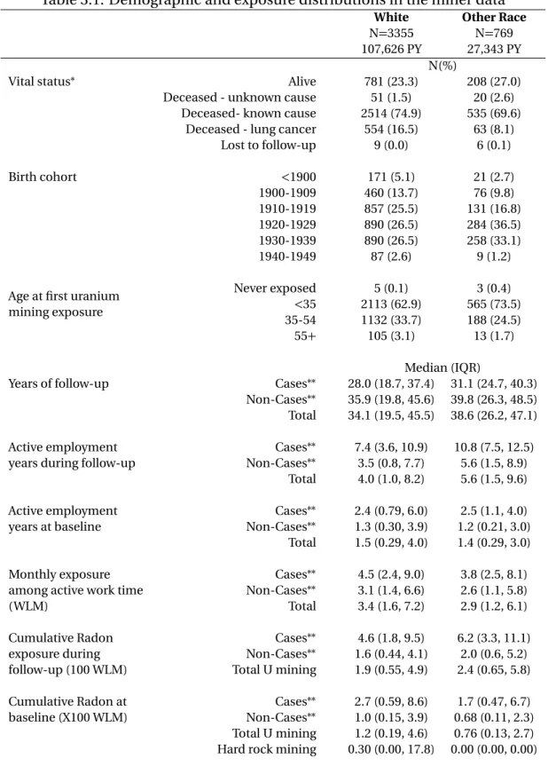
3.1 Demographic and exposure distributions in the miner data . . . 56

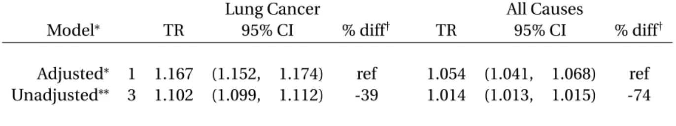
3.2 Time ratios and 95% confidence intervals per 100 working level months, 5 year lag. Male uranium miners, Colorado Plateau, USA 1950-2005. . . . 57

3.3 Time ratios and 95% confidence intervals for windows of exposure from adjusted model for lung cancer . . . 58

3.4 Sensitivity analysis for the change in the TR of the radon/lung cancer association by excluding short to long term prevalent hires in the study cohort. . . 59

3.5 Mean outcome(E[Y])by cumulative exposure PXk

and employment status(L2)in a hypothetical occupational cohort . . . 68

3.6 Mean outcome (E[Y]), stabilized inverse probability weights (S Wx₎

and pseudo-population cell sample size by strata of exposure (X1,X2) and employment status (L2) in a hypothetical occupational cohort . . . . 70

3.7 Mean outcome (E[Y]), stabilized inverse probability weights (S Wx₎

and pseudo-population cell sample size by strata of exposure (X1,X2) and employment status (L2) in a hypothetical occupational cohort in which exposure is measured off work (and positivity holds) . . . 74

3.8 Results of analysis on synthetic data from table 2 and table 3 . . . 74

A.1 Notation used to refer to quantities in the Colorado Plateau Uranium Miner (CPUM) data . . . 92

A.2 Structural nested model results for simulations: large sample charac-teristics . . . 106

A.4 Comparing alternative exposure models for SNAFT model for the radon-lung cancer dose-response . . . 109

A.5 Sensitivity analysis: alternative SNAFT models for quantifying the healthy worker survivor bias . . . 115

A.6 Comparing SNAFT model with parametric AFT model . . . 117

B.1 Continuity correction as an attempt to salvage causal effects in data subject to nonpositivity - continuity correction for weights only . . . 130

B.2 Continuity correction as an attempt to salvage causal effects in data subject to nonpositivity - continuity correction for both weight and marginal structural model . . . 131

LIST OF FIGURES Figure

1.1 222_{R nDecay Chain from}238_{U or}234_{U. Thoron (}220_{R n) and acton (}219_{R n)} produce different progeny. . . 2

1.2 Causal diagram showing causal relationships possibly underlying healthy worker survivor bias in a hypothetical occupational studies with nota-tion given in Table 1.2. . . 12

1.3 Causal diagram showing causal alternative relationships possibly un-derlying healthy worker survivor bias with notation given in Table 1.2. Employment directly affects the outcome of interest. . . 14

1.4 Figure 1 fromBjör et al.(2013) showing negative trends in multiple out-comes with employment duration in an iron mine . . . 16

1.5 Directed acyclic graphs comparing a model for healthy worker survivor bias (dashed arrow is present) with a model for the healthy hire effect (dashed arrow is absent) . . . 17

1.6 Causal diagram showing assumption under which a 1 unit exposure lag controls confounding by employment status . . . 27

2.1 1443 measured radon concentrations in 48 Colorado counties from 1986-1987 by the High-Radon Project, Lawrence Berkeley National Labora-tory (Price et al.(2011)) . . . 42

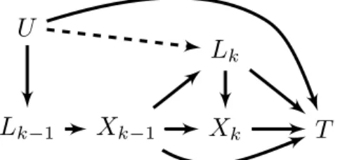
3.1 Causal diagram showing hypothesized relationships that necessitate use of special methods to control healthy worker survivor bias in the Colorado Plateau Uranium Miners data. Xk is radon exposure andLk

is active employment status in monthk. . . 49

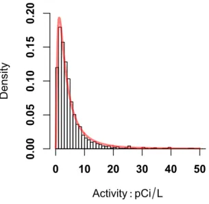
3.2 Illustrative monthly exposure distributions for white males born from 1920-1929 up to 35 WLM. Months selected represent the 5th, 50th, and 95th percentile for the mean monthly exposure from 1950-1969. Lines of fit are for visualization only and do not represent actual fit of sure models. Lines below histogram represent actual monthly expo-sures for individual miners. . . 55

3.4 Bias tradeoff between nonpositivity and measurement error in the anal-ysis of miner data; Top panel) Hazard ratio per 100 working level months from marginal structural Cox model (MSM) by imputed log-geometric mean of residential exposures, with grey reference line at the crude HR with no exposure imputation; Bottom panel) Mean inverse probabil-ity of exposure weights used in marginal structural Cox models by im-puted log-geometric mean of residential exposures . . . 77

A.1 G-function for SNAFT model for lung cancer mortality reported in §3.1 99

A.2 G-function for SNAFT model for all cause mortality reported in §3.1 . . . 100

A.3 Frequency of interval (days) between exposure readings in source data from Colorado Plateau Uranium miners data. Inset is histogram show-ing conditional distribution of intervals less than 1000 days (the largest bar in the primary figure). . . 111

A.4 G-function using a grid search algorithm for a simulated data set for 50,000 individuals. The figure shows data from the fully-adjusted linear model (Row 1 in table A.2). . . 113

A.5 Percentiles of cumulative radon exposure by age and ages of lung can-cer deaths (rug plot) in the miner data. . . 119

A.6 Distribution of age at death from lung cancer (gray bars), and potential age at death from lung cancer or artificial censoring under no exposure (black outlined bars) in the miner data. . . 119

A.7 Distribution of age at death from any cause (gray bars), potential age at death from any cause or artificial censoring under no exposure (black outlined bars) in the miner data. . . 120

A.8 Calendar time distribution of pre-follow-up employment time (black), employment time under observation (medium gray) and post-employment time (light gray) in the miner data - each horizontal line represents a single miner. The lines are grouped according to vital status at exit from the study. . . 124

A.9 Age distribution of pre-follow-up employment time (black), and time under observation (gray) - each horizontal line represents a single miner. The lines are grouped according to vital status at exit from the study. . . 126

LIST OF ABBREVIATIONS

AFT Accelerated failure time

BEIR Biological effects of ionizing radiation Bq Becquerel

CEA Commissariat á l’énergie

COGEMA Compagnie Générale des Matiéres Nucléaires CPUM Colorado Plateau uranium miners

ERR Excess relative risk/rate HR Hazard ratio

HWSB Healthy worker survivor bias

IARC The International Agency for Research on Cancer ICRP International Commission on Radiological Protection IP, IPW inverse probability, inverse probability weights LET Linear energy transfer

LNT Linear-no threshold

MSM Marginal structural model

NCRP National Council on Radiological Protection RR Relative risk/rate

SI The International System of Units (Le Système International d’unités) SNAFT Structural nested accelerated failure time

TSE Time since exposure

UNSCEAR United Nations Scientific Committee on the Effects of Atomic Radiation USEPA United States Environmental Protection Agency

WL Working level

CHAPTER I: INTRODUCTION

1.1 Radon

1.1.1 Public health significance

Elemental radon is a naturally occurring gas at room temperature and is carcino-genic to humans when it is part of the breathing air due to the radioactivity of both radon and its progeny (IARC(2012)). The most common isotope,222R nand its progeny shown in Figure 2 1.1 contribute most of the radiation dose (IARC(1988, 2001);ICRP

(2010); Chen et al. (2014)). Because radon is ubiquitous in air, soil, and water and concentrates in indoor air, there is substantial exposure potential in populations who spend time indoorsNRC(1999). This problem may be compounded by the use of cer-tain building materials, which also release radon (Gierl et al.(2014); Zhukovsky and Vasilyev(2014)).

222_{R n has an unstable nucleus and decays with a half-life of around four days by}

tissue, such as lung tissue.

The Committee to Study the Biological Effects of Ionizing Radiation (BEIR VI com-mittee) estimates that radon in indoor air is the second leading cause of lung cancer and plays a role in 15,000 to 22,000 lung cancer deaths per year in the United States, though risk projections are consistent with estimates from 3,000 to 33,000 (NRC(1999)). Unfortunately, increasing energy efficiency in homes may be resulting in an increase in indoor radon concentrations (Jiránek and Kaˇcmaˇrikova(2014);Yarmoshenko et al.

(2014)), which may exacerbate this problem. Importantly, radon exposures can be re-duced through measures such as home radon mitigation (Steck(2012)). Thus, the pub-lic health impact of radon on lung cancer is high, we may be heading towards an in-crease in the average population exposure, but there are possible interventions that can help reduce the burden of health impacts from radon exposure. However, because radon mainly comes from the soil, we can realistically only hope to reduce, rather than eliminate exposure, so epidemiologists have a role in estimating the public health im-pact of radon.

Radium 226 Radon 222 3.82d Polonium 218 3.05m (Radium A) α Short lived radon progeny (Historical names) Astatine 218 2s β Lead 214 26.8m (Radium B) α Radon 218 0.035s β Bismuth 214 19.7m (Radium C) α Polonium 214 0.000164s (Radium C) α β β Thallium 210 3.1m α Lead 210 22y α

β Bismuth 210 5d β Mercury 8m α Polonium 210 138d β Thallium 4m α Lead (stable) α β β Uranium 238/234

As noted above, there are many lung cancer deaths in the US that are possibly at-tributable to radon. However, radon exposure occurs over the entire life course, and biologically meaningful exposure can potentially occur over that whole period. Thus, the health effects of radon are difficult to study without having some measurement or estimate of radon exposure over a long period of time. Factors such as the age at ex-posure, the intensity or rate of exex-posure, the duration of exex-posure, and smoking may all modify the degree to which radon exposure increases the rate of lung cancer (NRC

(1999)), which only increases this difficulty. To simplify the analysis, radon exposure has often been operationalized using a time-integrated metric of exposure, such as cu-mulative exposure. Cucu-mulative exposure combines exposure rate with exposure dura-tion to form a single summary measure across time.

1.1.2 Lines of research of the public health impact of radon on lung cancer inci-dence and mortality

Substantial work has been done to model the population impact of radon expo-sure and cancers in the respiratory tract and lungs, which are the primary expoexpo-sure sites for radonICRP(1993). Generally, the lines of research into models of radon car-cinogenesis have followed one of three approaches: 1) an empirical or statistical mod-eling approach, which is focused on explaining macro-level trends in radon induced lung cancer, such as dose-response, dose-rate effects or empirical induction periods, 2) mechanistic modeling, which seek to link observed data directly to biologic processes using biologic models for the observed data (e.g. Richardson(2009a)) or 3) the dosi-metric approach, which involves extrapolating radiation dose-response curves from other ionizing radiation (particularly those derived from the atomic bomb cohort in Japan, e.g.Preston et al.(2007)) (NRC(1999)).

1.1.2.1 Miner studies of the radon-lung cancer association

The epidemiologic literature on the radon-lung cancer association in miners has a long history and spans multiple countries with large cohort studies of underground miners, such as those from Canada (e.g. Lane et al.(2010)), the Czech Republic (e.g.

Tomásek(2011)), France (e.g. Rage et al.(2012)), Germany (e.g. Kreuzer et al.(2012)), Sweden (e.g.Jonsson et al.(2010)) and the United States (e.g.Schubauer-Berigan et al.

(2009)). Several pooled analyses of these (and other) cohorts have been performed in an effort to increase the precision of association parameters (Lubin(1994);NRC(1988, 1999);Leuraud et al.(2011);Fornalski and Dobrzynski(2011)). The Committee on the Biological Effects of Ionizing Radiations from the National Research Council (United States) periodically releases summary reports of scientific literature on the health risks due to radiation, including the two reports on the risk of lung cancer due to radon in miners given inNRC(1988) andNRC(1999). The United Nations Scientific Committee on the Effects of Atomic Radiation (UNSCEAR) have summarized miner data in a re-port to the General Assembly (UNSCEAR(2008)). Additionally, the International Com-mission on Radiological Protection (ICRP) has released two summaries of epidemio-logic data pertinent to the radon-lung cancer associationICRP(1993, 2010), which are shown in Table 1.1 (adapted fromICRP(2010)). Each publication provided a table with the major summary estimates of the excess relative risk per 100 working level months (WLM - defined as any combination of exposure rate in working levels[130,000 MeV of potential αenergy per liter of air] and employment time that leads to an average exposure of 1 working level over 170 hours).

a reason for heterogeneity in results. The BEIR VI committee was able to estimate the modification of the ERR by age at exposure, duration of exposure, and exposure rate, however, and came up with a set of preferred models, discussed in §1.3 of the current manuscript. In the following, we discuss another possible source of heterogeneity that may derive from differences between cohorts in the complex relationships between employment and health.

1.2 Healthy worker survivor bias

1.2.1 Description

Radon is one of many occupational agents that may have persistent negative effects on health. Exposure from the past may have an effect on current disease status. Ex-posure duration may also play a role in disease as cellular repair pathways from prior insults may be overburdened and not able to cope with more recent insults. One way of approaching analyses of the health effects of such agents is to aggregate exposure to them over time. Within the miner literature, cumulative exposure to radon, duration of exposure, average exposure, or exposure accrued within specific time windows are all examples of such aggregation. While these are all simplifications of a complex, dy-namic process of how exposure may change over time, they are nonetheless very useful for summarizing the effects of exposures and for projecting the effects of exposure in other populations who have long term exposures.

health outcomes. This process is referred to in the occupational epidemiologic litera-ture as healthy worker survivor bias (Buckley et al.(2014)).

Healthy worker survivor bias has been traditionally considered simultaneously with a second bias, the healthy hire effect. This second bias describes a cohort selection process whereby unhealthy individuals are less likely to enter into employment ( Ar-righi and Hertz-Picciotto(1994, 1993)). Often, these biases are considered as a part of a single process termed the healthy worker effect. Both of these aspects of the healthy worker effect can be seen as specific instances of unmeasured confounding (Breslow and Day(1987)), but their unique characteristics and apparent ubiquity warrant spe-cial treatment here.

The healthy hire effect describes an unmeasured difference in health status be-tween the working population and the target population for inference. Because of this, comparisons of disease rates between occupational cohorts and other populations can yield biased estimates of effects of occupational exposures. This issue is circumvented through internal analyses of occupational groups, in which rates of disease are com-pared across exposure levels within the cohort. If exposure is well characterized, in-ternal analyses can result in an estimate of the dose-response – how the disease rates change over increments of exposure – which can inform occupational limits and public health efforts. However, effect estimates from internal analyses can be subject healthy worker survivor bias.

worker survivor bias is a structural component to occupational studies and would be expected in any study of the health effects of aggregated exposures within a dynamic workforce. Further, under certain models, healthy worker survivor bias is intractable to conventional statistical methods and may require more advanced approaches ( Ar-righi and Hertz-Picciotto(1994, 1993);Flanders et al.(1993);McNamee(2003);Pearce et al.(2007)).

1.2.1.1 Notation

Table 1.2: Notation used in this document referring to observed quantities

Variable∗ _{Interpretation Examples}

k A particular point in time Age 30, 1930

Xk Exposure of interest at timek∗∗ Radon exposure at age 19

¯

Xk Exposure history at timek∗∗ Annual exposures up to age 30,

Monthly exposures from 1955 to 1960

¯

Xk Summary exposure history∗∗ Cumulative radon exposure up to

age 30, Mean exposure up to age 30, Exposure duration up to age 30

Lk Study covariates at timek∗∗ Employment status at age 19, Job

title in 1930

¯

Lk Covariate histories at timek∗∗ Employment duration at age 19,

Number of jobs worked by 1930

V Study covariates fixed in time within the study†

Age at hire, birth cohort, race

T Time to event of interest Age at death from lung cancer

U Unmeasured variables Underlying health status, frailty, smoking (if unmeasured)

Note: all subscripts denoting individuals are suppressed for clarity

∗ _{Bolded variables refer to a possible vector (e.g. the collection of race, birth cohort,}

and age at hire), non-bold variables refer to a scalar (e.g. cumulative exposure at age 40), while lowercase variables refer to a realization (e.g. 10 WLM of exposure)

∗∗_{Also referred to as time-varying covariate}

1.2.1.2 A model for healthy worker survivor bias based using directed acyclic graphs

Robins (1986) proposed that healthy worker survivor bias could be (partially) ex-plained by a general set of causal mechanisms in occupational studies and showed that, under this assumed model, that conventional statistical methods cannot ade-quately reduce the amount of bias that results from these mechanisms. He posited that healthy worker survivor bias occurs when:

1. Employment status (whether or not at work) is an independent population risk factor for a disease outcome of interest, possibly because of association through an unmeasured health determinant that affects both employment and the out-comeU.

2. Previous employment status affects subsequent exposure (for example, if expo-sure only happens at work)

3. Previous exposures impact the rate of leaving work

Using the language of directed acyclic graphs (hereafter causal diagrams), we can formally express these relationships using simple graphs (Pearl(1995);Greenland et al.

(1999)). These diagrams allow a simple assessment of conditional dependence of a set of variables of interest - typically these variables are the exposure of interest, the out-come of interest, and all known confounders of the exposure-outout-come association. The causal diagrams are formal representations of graph-theory, which allows a for-mal assessment of possible structural biases (Greenland and Pearl(2008)) and can be extended to other situations such as bias due to missing data (Daniel et al.(2011)).

a possible mechanism underlying healthy worker survivor bias proposed byRobins

(1986).

X

U

L

T

X

Figure 1.2: Causal diagram showing causal relationships possibly underlying healthy worker survivor bias in a hypothetical occupational studies with notation given in Ta-ble 1.2.

This diagram can be used to show that regression based methods will be biased in this scenario. Using the variables shown in figure 1.2, consider a proportional hazards model of the form

λ(k|Xk,Xk−1,Lk) =λ0(k)exp(β1Xk+β2Xk−1+β3Lk)

Whereλ(k|Xk,Xk−1,Lk)is the hazard at timek conditional onXk,Xk−1,Lk, andλ0(t) is an unspecified baseline hazard for individuals at the referent level of each variable. The vector ofβparameters represent the log hazard ratio for a one unit change in each variable, while holding the other variables constant.

We are interested in estimating the effects of exposureX¯k ≡(Xk,Xk−1)on the haz-ard or time to death. That implies we are primarily interested inβ1 andβ2. The di-agram shows that there is confounding of theXk →T association along the pathway

Xk ←Lk →U →T. This is how the healthy worker survivor bias can be

conceptu-alized: confounding that occurs because a common factor causes both attrition from the workforce and the outcome of interest. This is often referred to as time-varying, or time-dependent confounding (Robins(1992);Daniel et al.(2013)).

In our model, we can control this confounding by includingLkin the model.

Lk is referred to as a collider on the path betweenXk−1andk because, along the path

Xk−1→Lk ←U →T, two arrow heads “collide” atLk. Adjusting forLk in this model

will up a non-causal, backdoor path from exposure to outcome, a situation known as collider bias (Cole and Hernán(2002);Greenland(2003);Cole et al.(2010)).

To see this bias, consider an individual at timek. Prior exposure and poor health can both cause individuals to leave work, so if that individual is off work, we know he either likely to be highly exposed or of poor baseline health. If he is unemployed and highly exposed, he is more likely to have good health and less likely to suffer the outcome of interest. Thus, within strata of employment, exposure and the outcome are associated, even if there is no effect of exposure on the outcome.

More relevantly, collider bias will still occur if we consider cumulative exposure (Xk−1+Xk) as the exposure of interest (or any summary of both time-specific

expo-sures). That is equivalent to our model above if we add the restriction thatβ1 =β2. Because we know thatβ2is biased if we adjust forLk, andβ1is biased if we do not ad-just forLk, the association between cumulative exposure and the outcome will also be

biased . Note that, had we measuredU, we could control this confounding by adjust-ing for it in the model, instead ofLk. Given the limited nature of occupational data,

which is often limited to employment records, it is unlikely that we could adequately captureU in most circumstances.

Bias would also occur if employment status directly affected the outcome (figure 1.3, say, by an increase in smoking after leaving a non-smoking workplace, or a loss of insurance benefits), and bias would be present even if exposure did not have an effect on the outcome (Rosenbaum(1984)). This bias occurs because Lk is an

intermedi-ate betweenXk−1and the outcome, so adjusting for it would be equivalent controlling some of the effect of exposure.

vary-Xk

Lk

T

Xk

Figure 1.3: Causal diagram showing causal alternative relationships possibly underly-ing healthy worker survivor bias with notation given in Table 1.2. Employment directly affects the outcome of interest.

ing confounder, or 2) bias from improperly accounting for employment status. The observed bias when considering cumulative exposure is generally downward because low cumulative exposures result from individuals leaving work who have a poor prog-nosis. Adjustment through conventional means may also yield a downward bias, how-ever, since it is conditioning out part of the total effect of exposure. Thus, based only on the simple model shown in figure 1.3 one might conceivably adjust for employment status in a regression model and see no change in the effect estimate because one bias has been traded for another.

1.2.2 Evidence of a possible healthy worker survivor bias in occupational radon studies

Healthy worker survivor bias has historically been of concern only when it results in benign or deleterious exposures appearing to be beneficial. For example, in a co-hort of Swedish iron-ore miners,Björ et al.(2013) observed negative trends in multiple outcomes with increasing employment time and employment time underground, as shown in Figure 1.4. These trends occurred even though the miners are exposed to radon, silica, and diesel exhaust, and dust in the underground environment - previ-ous analyses found associations between cumulative radon exposure and lung cancer (Jonsson et al.(2010)). The negative association between employment time and rectal cancer may be present due to beneficial effects of the physical activity inherent in min-ing (Slattery(2004)), but the positive effect of physical activity is not strong enough to induce such associations. Thus, there is evidence of healthy worker survivor bias in a cohort of radon exposed miners, but it may not be apparent with respect to lung can-cer because radon has highly specific effects and the effects are large enough to out-weigh any downward bias. This bias may be of little concern when testing hypotheses about highly deleterious exposures. However, when one is interested in characterizing a dose-response, healthy worker survivor bias should be considered a potential prob-lem even if it does not completely eliminate apparent associations.

1.2.2.1 Health related selection is observable in miner cohorts

FIGURE 1.

Mortality, Cancer and Iron-Ore Mining 535

the industry under study. The dashed arrow in Figure 1.5 represents the difference be-tween these two biases. Healthy worker survivor bias suggests that underlying health statusU affects employment status at all time points (i.e. the dashed arrow in figure 1.5 is present). When the healthy hire effect (and not healthy worker survivor bias) is present, thenU affects employment status only at timek −1 (the dashed arrow is absent). This diagram is an obvious over-simplification of the complex forces that drive employment changes across time. However, it highlights the similarity of the two sources of bias in occupational studies and clarifies the specific conditions under which one could observe a healthy hire effect but expect no healthy worker survivor bias.

T

U

L

L

X

X

Figure 1.5: Directed acyclic graphs comparing a model for healthy worker survivor bias (dashed arrow is present) with a model for the healthy hire effect (dashed arrow is ab-sent)

Often, standardized mortality ratios (SMRs) are interpreted as evidence of the healthy hire effect if they are below one. Deleterious effects of occupational exposures may counterbalance this effect, and strongly deleterious exposures may cause an excess of mortality in working populations. In an early analysis of the Colorado Plateau ura-nium miners,Archer et al.(1976) estimated an all cause SMR of 0.86 for American Indi-ans, with an SMR for heart disease estimated to be 0.10, and a deficit of mortality from non-accidental, non-respiratory causes among white miners.Schubauer-Berigan et al.

of circulatory diseases (SMR=0.65), non-lung cancer respiratory diseases (SMR=0.75), and non-respiratory cancers (SMR=0.80), while the all cause mortality SMR of 1.03 suggests that occupationally related diseases (e.g. accidents, SMR=1.86 and lung can-cer, SMR=1.90) may be masking a healthy hire effect in this population. The low SMR for non-lung cancer respiratory diseases remained in deficit in the most recent update of this population (SMR=0.80) while the all-cause mortality SMR remained near unity (SMR=0.97) (Lane et al.(2010)).

Stayner et al. (2003) attributes non-linearity observed Colorado uranium miners (seeHornung and Meinhardt(1987)) and in Czechoslovakian uranium miners (seeSevc et al.(1993)) to a lower than expected risk at high exposure levels. Because the phe-nomenon is not generally observed in miner studies (seeNRC (1999)),Stayner et al.

(2003) posited that non-linearity results from particular aspects of the cohorts under study, such as measurement error or healthy worker survivor bias. In an analysis of non-respiratory cancers in 11 underground miner cohorts,Darby et al.(1995) noted that, both within each cohort and in the joint analysis, SMRs were nearly all higher for workers that had been employed at least 10 years versus those employed fewer than 10 years, indicating some health related selection. NRC (1999) have noted the non-linearity at high exposures but addressed it by truncating person-time-at-risk when individuals reach the highest exposure levels. Thus, there is reason to suspect that het-erogeneity in the ERR/WLM from the miner studies may result partially from healthy worker survivor bias, which may be stronger in some cohorts.

1.3 Models of the dose-response relationship between radon and lung cancer

the radon-lung cancer dose-response and comment on the implications for healthy worker survivor bias.

Case reports of respiratory diseases in miners date back to Paracelcus (seeJacobi

(1993) for a history). However, uranium miner cohort studies did not begin in earnest until the 1960s. Since that time the radon-lung cancer dose-response has been exten-sively studied. Recent efforts have focused on estimating a dose-response at the “low” radon concentrations observed in residential settings using meta-analysis or pooled data from miners studies (e.g. Lubin(1994);Lubin et al.(1995a, 1997);Leuraud et al.

(2011)), residential studies (e.g. Lubin and Boice (1997); Lubin(2003);Krewski et al.

(2005, 2006)), a combination (e.g. Fornalski and Dobrzynski (2011)), or specific sub-groups of miners or residential populations (e.g.Lubin et al.(1994)).

Much work has been put into creating parsimonious models of the radon-lung can-cer dose response that follow basic principles. One of these principles, the linear-no-threshold(LNT) assumption, is common to many radiation studies. This assumption implies that the dose-response between radon and health outcomes will be linear and that exposure to radon at any level will increase the risk of adverse health outcomes (seeBrenner and Sachs(2006) for review of the mechanistic basis for the LNT).

The Committee on the Biological Effects of Ionizing Radiation VI (BEIR VI) (based on models developed byLubin(1994)), chose to model the radon-lung cancer associ-ation using a linear excess relative rate (ERR) model, shown in equassoci-ation 1.1.

λ(k|X¯_k−5;β) =λ0(k)(1+βX¯k−5) (1.1)

distribution, or it may be left unspecified as in a semi-parametric Cox proportional hazards model. This model can be expressed equivalently as

E R R(X¯k−5;β) =βX¯k−5 (1.2)

For risk projections, the authors of the BEIR VI report considered categorical ver-sions of both the “exposure-age-duration” and “exposure-age-concentration” models (known collectively as the BEIR VI modelsNRC(1999), p. 80). The BEIR VI models al-lowed for the ERR to vary over categories of time since exposure attained age and either exposure duration (cumulative up to timek) or exposure concentration (average up to timek) as in

E R R(X¯k−5L¯k1, ¯Lk2;β,θ,φ,γ) =β(X¯k−[5,15)+θ1X¯k−[15,25)+θ2X¯k−25)×φLk1×γLk2 (1.3)

whereX¯k−5= (Xk−[5,15),Xk−[15,25),Xk−[25+))is the exposure to radon in working level months

for the period 5-15 years, 15-25, or 25+years years prior. There is modification of the ERR by attained age ¯Lk1, and ¯Lk2can be either exposure rate (in working levels) or expo-sure duration. The coefficientβis the ERR/WLM at the reference level of all modifiers, theθ parameters represent the factor by which the ERR/WLM is multiplied for the time-window specific exposure, andφandγ are the factors by which the ERR/WLM is multiplied for their respective covariate. This model is equivalent to fitting a model with the three windows of exposure within strata of each of the time-varying factors, but the model given in gives explicit parameters for the strength of effect measure mod-ification by the time varying factors. Note that the model assumes that exposures in the previous five years have no effect on lung cancer outcomes (i.e. they assumed a five year lag).

which differs from the BEIR VI models only in that time since exposure is not consid-ered to modify the relative risk of lung cancer by radon exposure.

While the BEIR VI models include factors that multiply the ERR on a linear scale, there is no restriction on the modification. For example, in the model shown in 1.3, there is no restriction onφ, so strong modification by exposure rate could lead to the estimate of a negative ERR.

To get around this issue, other models were developed in which which modifying factors (e.g. time since exposure) are considered to have a log-linear relationship with the relative risk of lung cancer. For example, in a cohort of Canadian uranium workers,

Lane et al. (2010) and in a joint analysis of French and Czech minersTomásek et al.

(2008) considered (in addition to the BEIR VI “exposure-age-concentration” model), models of the general form

R R(X¯5,L¯k;β,γ) =1+X¯5βexp L¯kγ

(1.4)

This model allows modifiers to enter the model as linear terms (rather than categorical as in the BEIR models) - otherwise, a linear trend may predict a negative ERR for certain combinations of exposure and the modifiers.

Leuraud et al.(2011) considered a model that further generalizes that in 1.4 by

al-lowing for modification of the baseline rate (at the reference level for all exposures and modifiers) by fitting a model of the type

R R(X¯5,L¯k,Sk;β,γ,θ) =exp(Skθ)

1+X¯5βexp L¯kγ

(1.5)

WhereSk in the study was current smoking status. Note that forβ=0 this corresponds

to a standard log-linear rate model.

the simple model given in 1.2. An equivalent approach has been applied to the rela-tionship between smoking and lung cancer (Vlaanderen et al.(2014)) as an attempt to improve on the pack-years metric (Thomas(2014)), which is the analog of the cumu-lative exposure used in the radon literature.

A shortcoming of each of the models 1.3-1.5 is that the modifiers they consider are restricted to modification by historical summaries or current values of the modifiers. Generally, historical summaries are needed for factors such as exposure rate (e.g. av-erage exposure rate up to agek) and age at exposure (e.g. age at median exposure) because mortality generally does not occur until long after exposure has ceased.

As a more general approach to modeling the time-related aspects of exposure his-tory,Richardson et al.(2012) considered an approach that was not a simple variation on the models 1.3-1.5. Rather than considering how time related aspects of exposure might modify the effects of cumulative exposure, the authors considered how these factors might modify the cumulative exposure itself. In this model, given in 1.6, the summary exposure metric changes with modifying factors. The summary metric can be considered a time varying weighted sum of exposurePk

u=0X¯uwu, such that when

the weightw¯k = (w0, ...,wk)is always one, this summary metric is equal to the

cumula-tive exposure. Otherwise, this weight varies as a function of the collection of modifiers included inL¯k and the parameter vectorγ, which quantifies the strength of this

mod-ification.

E R R(X¯k,L¯k;β,γ) =1+ k

X

u=0 ¯

Xuβexp L¯uγ

(1.6)

consider some time-varying summary of exposure history to be the relevant predic-tor of lung cancer mortality, rather than, say only current exposure. When some of these potential modifiers may also be confounders, however, this set of approaches may be biased. As shown in §1.2.1.2, if exposure at prior time points can affect the subsequent evolution of these modifiers, then bias will result. For example, if prior ex-posure influences the rate of leaving employment, then models that do not stratify by some function of employment history may be biased due to confounding. However, models that stratify by such factors - including exposure duration, which is strongly affected by employment history - will also be biased. Thus, the possible presence of healthy worker survivor bias in studies of radon exposed populations motivates the need for models that can account for a time-evolving exposure while not being subject to the shortcomings of regression models. We explore such models in the next section.

1.4 Existing analytic methods proposed for reducing bias due to healthy worker survivor bias

1.4.1 Parametric g-computation algorithm

P r(A=1) = X

b∈(0,1)

P r(A=1_|B=b)×P r(B=b) (1.7)

Unlike the representation of the ERR model in equation 1.1, this way of express-ing standardization requires use of discrete time - and slightly different notation. In this case, the outcome of interest is an outcomeDk that is measured at discrete points

in time, such as a study visit. We define the g-formula using a simple data structure in which, at timek exposure (Xk), employment status (Lk), and the death (Dk) are all

dichotomous variables. The cumulative incidence, Ik is the proportion of

individu-als who have died by timek. To estimate Ik we can factorP r(Dk =1)as in 1.7. The

standardized (marginal) cumulative incidence (Ik) of the dichotomous outcome Dk

(assuming no censoring) can be expressed using the g-formula as:

Ik=P r(Dk=1) = (1.8)

k

X

j=1 X

l

X

x

P r(Dj =1|X¯j =x¯j,L¯j=L¯j,Dj−1=0)×

j

Y

m=1

[P r(Xm=xm|L¯m =l¯m,X¯m−1=x¯m−1,Dm−1=0)×

P r(Lm =lm|L¯m−1=¯lm−1,X¯m−1=x¯m−1,Dm−1=0)×

P r(D_m−1=0|L¯m−1=¯lm−1,X¯m−1=x¯m−1,Dm−2=0)]

Where variables with subscripts_≤0 drop out ifm<=2.

The g-formula can be used for effect estimation by estimating the cumulative inci-dence under different interventions on exposure. For example,Ix¯k

k is the cumulative

incidence at timek we would expect under the interventions e t(X¯k =x¯k). The

cumu-lative incidence under an intervention is estimated using the g-formula by replacingx¯k

risk difference at timek for always versus never exposed, we can take the difference between two interventionsI¯1

k-I

¯ 0

k.

Non-dichotomous data, moderate to small sample size and extended follow up (i.e. any condition that results in sparse strata) necessitate use of models and Monte Carlo sampling. This approach is referred to as the parametric g-formula (see examples in

Robins et al.(2004);Taubman et al. (2009); Westreich et al.(2012);Cole et al. (2013);

Keil et al.(2014a)). Recently,Edwards et al.(2014) used the g-formula to estimate the effects on mortality of implementing and enforcing a series of different occupational limits on exposure in the study population used in the analyses in chapters 3.1 and 3.2, the Colorado Plateau uranium miners.

We note that the g-methods (the parametric g-formula, g-estimation of structural nested models, inverse probability weighted marginal structural models) originate in the causal inference literature and under the assumptions given in Appendix C.3 the parameters from these methods may have a causal interpretation. Without necessar-ily assuming we have identified a causal effect, however, g-methods have some advan-tages over standard regression models. Under the conditions for healthy worker sur-vivor bias outlined byRobins(1986), g-methods appropriately adjust for time-varying confounding in which some of the confounders are also intermediates. Namely, as shown with the g-formula examples, the parameter of interest is the marginal inci-dence under an interventionIx¯k

k . This marginal incidence is not stratified by the

time-varying confounder, so it does not fall prey to the pitfalls of stratifying or condition-ing on a variable affected by exposure that we noted in §1.2.1.2 and were discussed by

Rosenbaum(1984) andWeinberg(1993).

1.4.2 Other proposed solutions

compare them in an analysis of the association between arsenic exposure and cancer outcomes in a cohort of copper smelters, whileHertz-Picciotto et al.(2000) compare the methods using the same cohort in an analysis of the arsenic-cardiovascular disease association. Three methods were compared with the g-null test (an early g-method similar to the parametric g-computation algorithm - seeRobins(1987b)): exposure lag, adjustment for employment status, cohort restriction. Using causal diagrams we can show the specific conditions under which these analyses may control healthy worker survivor bias.

Exposure lag Gilbert(1982) employed use of an exposure lag to control healthy worker survivor bias under the rationale that the most recent exposures could only be accrued by employees that survived/stayed at work (namely, the healthiest employees). Under figure 1.6, this is equivalent to removing the arrowXk →T. Doing so, and not

includ-ingXk in the model for lung cancer, ensures that exposure is not confounded by Lk,

sinceLk only confounds theXk →T association. If there is, in reality, aXk →T

asso-ciation, then there will be induction of some measurement error due to the fact that were are ignoringXk. If we consider a more realistic setting, then there will be a likely

trade-off between measurement error due to ignored exposure and confounding by employment status that depends on the length of lag used.

In an analysis of the arsenic-lung cancer association, Arrighi and Hertz-Picciotto

should be noted that exposure lagging in this context is identical to exposure lagging to account for the empirical latency period between exposure and disease onset Roth-man(1981);Richardson et al.(2011). The results ofArrighi and Hertz-Picciotto(1996) could also be a consequence of modeling the disease process more effectively in mod-els using a lag that approaches the average empirical latency period in the cohort.

In a simple model of healthy worker survivor bias shown in figure 1.6, utilizing a lag of one unit of time would appropriately adjust for confounding by employment status without inducing additional bias. Using this diagram, confounding occurs alongXk←

Lk ←U →T, and by excludingXk (through the lag), we have eliminated confounding

of the effect of the exposure of interestX¯k = (Xk−1,Xk). This model requires that there

is no time-varying confounding ofX_k−1 →T and is not likely to hold in any realistic setting. Note that lags may still be appropriate to address disease latency, but analysis of our causal diagram in Figure 1.6 suggests that exposure lagging will not be sufficient to control healthy worker survivor bias. However, it may be useful in concert with other methods (e.g.Garshick et al.(2012),Naimi et al.(2014a)).

Xk

Lk

T

Xk

Figure 1.6: Causal diagram showing assumption under which a 1 unit exposure lag controls confounding by employment status

backdoor path between exposure atk and the outcome. Stratification on current em-ployment status would block confounding pathways forXt, but would also block part

of the total effect of exposure at time 1, thus biasing the estimate of total exposure. Additionally, this adjustment induces collider-stratification-bias by opening up a non-causal, backdoor pathXk−1→Lk ←U →T, whereLkmeans that the model was

strati-fied byLk (Greenland(2003);Cole et al.(2010)). If exposure does not affect subsequent

employment status - i.e. if exposure has no effect on health during employment, then stratification of person time would function to eliminate confounding by employment status (e.g. the causal diagram shown in figure 1.3). If the confounding throughLk is

strong relative to the indirect effect of prior exposure (X_k−1) throughLk, then

adjust-ment may increase effect estimates.Steenland and Stayner(1991) observed such an in-crease and concluded that employment status is an important variable for adjustment in occupational studies. Such an increase does not rule out collider bias, however.

A similar approach was proposed by Flanders et al.(1993), who explored an em-pirical model for the healthy hire effect in which they proposed adjustment for time-since-hire to reduces bias due to healthy worker effects. The authors also posited that the healthy hire effect faded over time through a mechanism in which the hazard in-creased in proportion to the number of years employed, suggesting that cumulative work (conditional on age) actually makes workers more sick. Interestingly, the authors observed a downward bias due in risk ratios (compared to employment duration ad-justed models) to their hypothesized set of effects, which is same as that seen by Steen-land and Stayner(1991) among several work forces.Cardis et al.(2007) observed a 0.31 ERR/Sv for radiation dose effects on all cancers (excl. leukemia) before adjustment by duration of employment and a 0.97 ERR/Sv after adjustment in the 15 country study of radiation exposed nuclear workers. These results conform to the theoretical direc-tion of bias due to healthy worker survivor bias in work byMcNamee(2003) andRobins

could be eliminated by adjusting for time-since-hire, butArrighi and Hertz-Picciotto

(1995) suggests using results from two cohorts that the empirical model of Flanders et al.(1993) does not hold due to apparent confounding of the time-since-hire effect by age and employment status.

Richardson et al.(2004) showed in simulations that bias patterns observed in healthy worker survivor bias could result from a strong correlation between cumulative expo-sure and time-since termination. The authors noted in simulations that large, spurious associations could be induced by simply adjusting for a binary indicator of employ-ment status, whereas adjustemploy-ment for time-since-termination returned the expected re-sult. The methods were replicated in a cohort of utility workers with the same pattern of results, and later applied byGarshick et al.(2008) to a cohort of trucking industry workers.Steenland and Stayner(1991) observed that the SMR during inactive (unem-ployed) person time was higher than that during employment, and a decrease in the SMR by duration of employment - the confluence of which is consistent with sick work-ers leaving, rather than employment increasing the health of employees. These results emphasize the importance of considering employment status as a time-varying factor in any occupational study, as well as considering a set of employment status “history” variables that could include time-since termination or duration of employment.

restricted to 10+or 15+.

In the causal diagram in Figure 1.6, this method can be expressed as restricting the cohort to those withL2=1. This restriction is fraught with the same issues as regres-sion adjustment forL2. Further, there is no reason to suspect that selection effects from healthy worker survivor bias are decreased at all in restricted cohorts, and it is impos-sible to disentangle posimpos-sible control of any healthy worker effects from the effects of selection bias induced by restricting analysis cohort that has a) survived long enough to be in the cohort and b) been subjected to more exposure than others.

The g-null test The g-null test was another approach developed byRobins(1986) to address healthy worker survivor bias when exposure may influence employment. This method is similar to g-estimation of structural nested models (discussed in §1.5.1), but is less general. The approach relies on creating nested matched sets individuals, where the matching is on exposure and covariate history. Each nested set is analyzed with the equivalent of a conditional logistic model where a case is defined as an individual who eventually dies of the disease of interest. The test was low powered, soRobins(1987b) developed a slightly more powerful version that was applied byHertz-Picciotto et al.

(2000) to study the effects of arsenic on circulatory disease. While the approach might be tenable for short term studies with only categorical covariates, it appears that g-estimation of structural nested models may offer the same advantages without any of the disadvantages of the g-null test.

Summary Robins’ model for healthy worker survivor bias is inclusive of many pre-viously suggested models (e.g. McNamee(2003);Flanders et al.(1993);Pearce(1992);

probability weighted marginal structural models. In Figures 1.2-1.5, if exposure does not influence subsequent employment, then adjustment for employment status would also be expected to remove confounding without introducing additional bias. Ulti-mately, these simplified scenarios are useful for suggesting approaches in certain sce-narios, but the often unobservable complexity of relationships between the external environment and health implies that we can only approximate the truth with models. The flexibility of g-methods makes them a useful tool to in a wider array of environ-ments than standard regression models.

1.5 Proposed solutions considered in this dissertation

Two methods aside from the g-formula designed for the study of exposure effects under time varying confounding are inverse probability of exposure weighted marginal structural models (MSM), and g-estimated structural nested models. Of these, inverse probability weighted Cox MSMs and structural nested accelerated failure-time mod-els (SNAFT model) have utility for data in which the effect of cumulative exposures on a binary outcome are of interest. Both models can potentially be used to control time varying confounding by employment status and employment history, which We hypothesize will control healthy worker survivor bias. We propose to apply these two methods, and We describe simple examples of them in §1.5.1 and §1.5.2.

1.5.1 Structural Nested Accelerated Failure Time models

pa-rameter, as with the parametric g-formula, and is not subject to the pitfalls of regres-sion models noted above.

A SNAFT model can be expressed in a simple case as

T¯0=

T

Z

k=0

exp(ψXk)d k (1.9)

WhereT¯0 _{is the failure time we would observe if the individual had never been} ex-posed. The parameter of interest exp(₋ψ)is interpreted as the factor by which expo-sure contracts one’s lifespan, For example, if exp(₋ψ) =1/2, exposure cuts the amount of potential time one could live in half - that is, the failure time observed under con-stant exposure is half that we would observe under no exposure. To account for time varying exposures, we have to integrate the exposure function over the observed time. This model allows us to calculate the potential failure time under no exposure using the data. For example, ifψ=0.2 for an individual with an observed failure timeT =2.2 and exposure historyX¯k = (1, 0, 1), the survival time under the exposure history “never

exposed” (X¯k = (0, 0, 0)) would be

T¯0 = e0.2∗1∗(1−0)years + e0.2∗0∗(2−1)years + e0.2∗1∗(2.2−2)years = 2.47 years

Estimation of the SNAFT model is done using g-estimationRobins(1989);Robins and Tsiatis(1992). A simple g-estimation algorithm would proceed as follows:

First, take a guess atψ(calledψe) and use equation 1.9 to generate a set of the po-tential failure times under no exposure atψecalledTe

¯ 0_{as in}

e

T0¯=

T

Z

k=0

exp(ψeX_k)d k.

Xk. This could be a logistic model such as

l o g i t[P r(Xk=1|VL¯k,X¯k−1,Te ¯

0_{,T >k;β,θ)] =β}

0k+Vβ1+L¯kβ2+X¯k−1β3+Te ¯

0_{θ (1.10)}

in which the dependent variable is the exposure at timek(Witteman et al.(1998);Hernán et al.(2005)). The model includes a interceptβ_0kthat may be time varying. Because the outcome we would observe under no exposure can only depend on exposure if there is unmeasured confounding (i.e.T0¯_{is treated as a baseline variable determined prior} to any exposure or covariates), if all confounders are accounted for in the right side of equation 1.10,Te

¯

0 _{will equalT}¯0_{when θ =0 (Robins(1989)). One can perform a grid}

search over a reasonable range ofψe, and theψethat yields a Z-statistic forθ equal to 0 (or very close to 0) is the estimate ˆψ. G-estimation is the term given to this search.

To develop some intuition, one could consider T0¯ _{to be the “residual” outcome} once the net effects (the parameter of interest) of exposure are removed. It is the vari-ation in the observed outcome that is not due to exposure. Theψparameter corre-sponds to this net effect. Once we have removed the variation in the outcome not due to exposure, then the residual outcome should be independent with an increment of exposure (Xk). We might expect that the residual outcome would vary between

indi-viduals with different employment and exposure histories, so we test for this indepen-dence within strata of these variables.

The formulation of a SNAFT model described in this section assumes that all out-comes are observed. This model requires modification when when some outout-comes are unobserved due to censoring. A description of the g-estimation of a SNAFT model in the presence of censoring can be found inWitteman et al.(1998), or inJoffe et al.

(2012) (the latter of which is more technical).

covariates. Using the estimating equation 1.10 as an example, note that occupational studies are sensitive to this assumption. If exposure cannot occur off of work, then the probability of exposure whenLk =0 (currently off work, a component ofL¯k ) will

always be zero. In such a case, the coefficientsβ₁,β₂andθ are not estimable in a sat-urated model.

G-estimation can overcome such violations of the positivity assumptions, provided we replace it with another assumption (Joffe et al.(2010)). An example of this assump-tion was given byChevrier et al.(2012), who used a modified estimating equation of the form

l o g i tP r(Xk=1|V,X¯k−1,Te ¯

0_{,T >k,L}

k =1;β,θ)

=β0k+Vβ1+X¯k−1β2+Te ¯ 0_θ

Where the estimating equation is only used on the person-years of active employ-ment in the data (Lk =1). Using occupational data, we can estimate all coefficients

in this model because there is no longer a violation of positivity. This amounts to a relaxation of the assumption of no unmeasured confounding (see appendix C.3) so that it only applies to the person time at work. Joffe et al.(2010) refer to this as a se-lective ignorability assumption and offer several examples in which, even though the assumption of no unmeasured confounding does not hold for all data, information from a subset in which it does hold (e.g. subsets with better exposure measurement or no missing covariates) can be leveraged to estimate causal effects with less bias than would be possible using the full data.

when nonpositivity may happen because of sparse data, such as in analyses of data with long follow-up and many potential confounders.

The validity of this approach relies on specification of the structural nested model and the model proposed for the estimating equation. This is fewer models than are required by the g-formula, but more than a standard regression approach. Most ex-amples of structural nested models in the literature are relatively simple models with dichotomous exposures (Joffe et al.(1998);Hernán et al.(2005);Chevrier et al.(2012);

Neophytou et al.(2014)) and there are relatively few examples of fitting SNAFT models with quantitative exposures (Joffe et al.(2012);Naimi et al.(2014a)). Even in simulated data, SNAFT models may not perform well in reasonably sized data sets (Young et al.

(2010)), andJoffe et al.(2012) noted difficulties with g-estimation when trying to es-timate multiple SNAFT model parameters. However, these models may complement standard regression models, and they appear promising for wider use in occupational studies to control healthy worker survivor bias (Joffe(2012)).

1.5.2 Marginal structural models

Robins and colleagues also described marginal structural models, another class of models that can adequately control for time-varying-confounders that mediate the exposure-outcome association (Robins(1997, 1999);Robins et al.(2000)). A marginal structural model is a tool for analysis that estimates associations between exposure and an outcome, much like standard regression models. They are relatively simple in implementation and provide parameters with familiar interpretation. Thus they are an attractive tool for epidemiologists.

to confounding, however, so this trivial model is not usually of interest. Assuming that all confounders are measured, one can estimate a marginal structural model using in-verse probability weighting (Horvitz and Thompson(1952)).

Returning to the notation used in previous sections (shown in table 1.2), these weights can be estimated using data via

ˆ

Wk= k

Y

j=0

P r[Xj =xj|L¯j =l¯j, ¯Xj−1=x¯j−1,V =v]−1

Informally, inverse probability weighting relies on the principal that the same types of individuals are present in both exposed and unexposed groups, but in different pro-portions that can be weighted to a common standard. The weights are applied to data so that each individual is represented by ˆWk copies in the data. The weighting results

in a “pseudo-population” in which confounders included in the weight model are bal-anced over the levels of exposure. An inverse probability weighted marginal structural model using weights ˆWkis just a crude model fit to the pseudo-population, rather than

the observed population.

A non-trivial example of using inverse probability weighting is to fit a marginal structural Cox proportional hazards model. For a binary exposure, this model esti-mates the change in the relative hazard for a one unit increase in exposure. Hernán et al.(2000) interprets the coefficient from such a model as the “ratio of the mortality (hazard) rate at any timet had all subjects been continuously exposed... compared with the hazard rate at timet had all subjects remained unexposed” (p 563). This def-inition has not been previously extended to a cumulative exposure.

The positivity assumption for inverse probability weighting Note that if

1/Wˆk = k

Y

j=0