ESSAYS ON ITERATIVE AND TWO-STEP ESTIMATORS WITH APPLICATIONS TO FINANCIAL ECONOMETRICS
David T. Frazier
A dissertation submitted to the faculty of the University of North Carolina at Chapel Hill in partial fulfillment of the requirements for the degree of Doctor of Philosophy in the Department of Economics.
Chapel Hill 2014
Approved by: Eric Renault Eric Ghysels David Guilkey Jonathan Hill
c
2014
ABSTRACT
DAVID T. FRAZIER: ESSAYS ON ITERATIVE AND TWO-STEP ESTIMATORS WITH APPLICATIONS TO FINANCIAL ECONOMETRICS.
(Under the direction of Eric Renault.)
ACKNOWLEDGMENTS
I am extremely grateful for the help and guidance I have received over the last few years. First and foremost, I would like to thank my dissertation advisor, Eric Renault, for his expert advice and direction over the last few years. I would also like to express my gratitude to Eric Renault for inviting me to visit Brown University, where, under his supervision, I was able to polish a large portion of this dissertation. I am indebted to my dissertation committee members, David Guilkey, Eric Ghysels, Jonathan Hill, and Saraswata Chaudhuri for sharing their time with me to discuss Econometric Theory and its application. I would like to personally thank Saraswata Chaudhuri for sparking my interest in Econometric Theory and for our many wonderful con-versations about life and Econometrics. I am thankful for the thoughtful comments I received from participants at the UNC Econometric Theory Workshop and the Brown University Econo-metrics Lunch Workshop; the insightful conversations and issues raised during these workshops contributed greatly to my overall understanding of the ideas presented in this dissertation.
TABLE OF CONTENTS
Table of Contents . . . v
List of Tables . . . viii
List of Figures . . . ix
1 Maximization By Parts in Semiparametric Models . . . 1
1.1 Introduction . . . 1
1.2 Framework and Estimators . . . 6
1.2.1 Framework . . . 6
1.2.2 Existing Estimators . . . 7
1.2.3 Maximization By Parts . . . 10
1.3 Examples . . . 15
1.3.1 Example One: GARCH-in-mean . . . 15
1.3.2 Example Two: Predictability in the Merton Credit Risk Model . . . 21
1.4 Asymptotic Properties . . . 31
1.4.1 Consistency . . . 31
1.4.2 Information Dominance Condition . . . 34
1.4.3 Asymptotic Normality . . . 36
1.5 Conclusion . . . 39
1.6 Tables . . . 41
1.6.1 GARCH-in-mean Example . . . 41
1.6.2 Credit Risk Example . . . 42
1.7.1 Existing Results . . . 43
1.7.2 Main Results . . . 43
1.8 Kernel Estimation . . . 50
1.8.1 Assumption 6 . . . 52
1.8.2 Assumption 2 and Assumption 7 . . . 53
1.8.3 Assumption 8 . . . 53
1.8.4 Assumption 9 . . . 53
2 The Shape of the Risk Premium Across Multiple Assets . . . 55
2.1 Introduction . . . 55
2.2 Semiparametric DCC GARCH-Mean Model . . . 59
2.3 Estimation . . . 63
2.3.1 Parametric Estimation . . . 63
2.3.2 Semiparametric Estimation . . . 64
2.4 Inference . . . 69
2.5 Empirical Application . . . 71
2.5.1 Data . . . 72
2.5.2 Estimation Results . . . 74
2.6 Conclusion . . . 75
2.7 Tables and Figures . . . 76
2.7.1 Tables . . . 76
2.7.2 Figures . . . 80
3 Two-Step Estimation Without Nuisance Parameters . . . 82
3.1 Introduction . . . 82
3.2 Efficient Two-Step Estimation . . . 85
3.3 Comparison With Existing Methods: Maximization by Parts(MBP) . . . 88
3.3.1 General Comparison . . . 88
3.3.2 Separable Likelihood Functions . . . 90
3.4.1 Alternative Representation. . . 95
3.5 Applications of Two-step Estimators . . . 97
3.5.1 Bivariate Gaussian Copula Models . . . 97
3.5.2 Merton Credit Risk Model . . . 104
3.6 Conclusion . . . 108
3.7 Polynomial Equations . . . 109
3.7.1 Copula Polynomial . . . 109
3.7.2 Merton Polynomial . . . 109
3.8 Tables . . . 111
3.9 Regularity Conditions . . . 113
3.10 Proof: 4 . . . 114
3.10.1 Proof: Theorem 5 . . . 116
3.11 Sequential Estimators . . . 119
3.11.1 Adaptive Estimation . . . 119
3.11.2 Nonadaptive Estimation . . . 120
LIST OF TABLES
1.1 GARCH-in-mean Model . . . 41
1.2 Monte Carlo Variance, Bias, and Mean Squared Error. . . 42
1.3 MBP Algorithm Estimates for the Merton Credit risk model. . . 43
1.4 Maximum Likelihood estimates under model misspecification. . . 43
2.1 Summary statistics for the monthly excess returns. . . 76
2.2 Global signal-to-noise ratios for the different portfolios. . . 77
2.3 Rolling signal-to-noise ratio for each portfolio in increasing order. . . 77
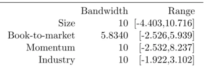
2.4 Estimated bandwidth and 90% range of the estimated conditional covariances. . 78
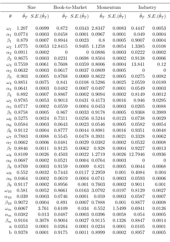
2.5 Parameter estimates for each portfolio with standard errors (S.E.(ˆθT)). . . 79
3.1 Gaussian Copula model estimates: low and medium correlation. . . 111
3.2 Gaussian Copula model estimates: high correlation. . . 112
3.3 Estimation Time (in seconds) across the different simulations. . . 112
LIST OF FIGURES
2.1 Risk premium for size, book-to-market, momentum and industry portfolios. . . . 80
2.2 Risk premium size portfolios with 95% confidence intervals. . . 80
2.3 Risk premium book-to-market portfolios with 95% confidence intervals. . . 81
2.4 Risk premium industry portfolios with 95% confidence intervals. . . 81
CHAPTER 1
MAXIMIZATION BY PARTS IN SEMIPARAMETRIC MODELS
1.1
Introduction
Many economic models depend on functions that are known up to a vector of finite dimensional parameters and other functions that are unknown but which are generally assumed to satisfy some smoothness conditions. The resulting models are called semiparametric since they combine parametric forms for certain components of the model with weaker nonparametric restrictions for other model components (Powell, 1994).
In this essay we investigate Maximum Likelihood estimation in semiparametric models where the log-likelihood function contains unknown finite dimensional parameters θand an unknown function, which we will often refer to as an infinite dimensional parameter,η that can depend on data and θ(or a subvector of θ). Throughout this research we illustrate the infinite dimen-sional parameter’s dependence on θ as η(·, θ). This specification for the model parameters is encountered in situations whereη depends onθ through some initial profile step and in situa-tions whereηdepends on covariates that are generated according to a parametric model, which depends on the parameters θ. There are many situations in economics and finance whereη de-pends on covariates that are generated according to an underlying parametric model. Examples include GARCH-in-mean models and many dynamic models with latent covariates; see Section 1.3 for two specific examples. Additional examples of semiparametric models with generated covariates can be found in Mammen et al. (2012) and Escanciano et al. (2013).
estimator (MLE) of θ can be computationally difficult, and in some cases infeasible. A po-tential means of bypassing this issue is to instead estimate θ using the well-known backfitting approach, which optimizes over the simple occurrences of θ in the log-likelihood and iterates over the complicated occurrences ofθin the log-likelihood. However, in the settings we are in-terested in analyzing the resulting backfitting estimator ofθwill be less efficient than the MLE of θ. This research proposes a new semiparametric estimation procedure that is as computa-tionally simple as backfitting but yields estimators that are always asymptotically equivalent to those obtained by Maximum Likelihood.
To clarify ideas, assume, for simplicity, we have some preliminary nonparametric estimator of η(·, θ) denoted ˆη(·, θ). Given the log-likelihood function
Lηnˆ(θ) = n X
i=1
`i(θ,η(ˆ ·, θ)),
where`iis the log-likelihood contribution for thei-th observation, the MLE ofθ, denoted ˆθn, can be obtained by solving the first-order conditions: ∂Lηn(θ)/∂θˆ = 0. The computational complex-ity associated with obtaining ˆθn can be seen by noting that even if a nonparametric estimator ˆ
η(·, θ) exists this estimator will depend on the parameters θ, potentially in a highly nonlinear fashion, and so directly solving the first-order conditions ∂Lηn(θ)/∂θˆ = 0 by simultaneously searching over every occurrence of θmay be cumbersome or impractical.
the NR algorithm, quasi-Newton algorithms could instead be used to estimateθ. While quasi-Newton algorithms are not required to calculate the full Hessian matrix, quasi-quasi-Newton methods are complicated by issues such as problem scaling and algorithm parameter selection. The Fisher scoring algorithm is yet another alternative. Fisher scoring works well so long as the sample size is reasonably large and the initial starting point is a consistent estimator, but for smaller sample sizes this method can be unstable because of variation in the estimated information matrix (Song et al., 2005).
If directly maximizing Lηn(θ) is difficult or infeasible an alternative is to estimateˆ θ using a backfitting approach. Unlike Maximum Likelihood, backfitting does not directly maximize over every occurrence ofθinLηn(θ). Instead, backfitting maximizes over the simple occurrences ofˆ θ inLηn(θ) and iterates over the complex occurrences ofˆ θinLηn(θ), most often the occurrence ofˆ θ in ˆη(·, θ). Compared with other estimation methods, such as Maximum Likelihood, backfitting can yield estimators that are substantially simpler to compute. The relative simplicity of the backfitting approach and its favorable computational properties have made backfitting one of the dominant estimation methods in semiparametric and nonparametric statistics. However, backfitting is not without its pitfalls. Because backfitting does not maximize over all occurrences of θ in Lηn(θ) the estimator forˆ θ obtained upon convergence of the backfitting iterations is generally inefficient (see Pastorello et al., 2003 and Hu et al., 2004 for examples). Simulation results also demonstrate that even in simple semiparametric models backfitting estimators can perform poorly in finite samples compared to Maximum Likelihood estimators (see, e.g., Hu et al., 2004 and Bravo and Jacho-Ch´avez, 2012).
because this method effectively assumes that, for a fixed θ, the parameter η is known” and so estimates of θ obtained by maximizing Lηn(θ) “can be misleading in both precision andˆ location.” Consequently, obtaining an accurate estimator ofθ in this setting may require more than just computing power; i.e., even if we have large amounts of computing power at our disposal existing estimation methods may still deliver a poor estimate of the trueθ.
The difficulties in obtaining a computationally simple and accurate estimator ofθstem from the infinite dimensional parameters dependence on θ. If an estimator for θ could be devised that somehow mitigates this dependence, either through a factorization of the log-likelihood function or by other means, it may be possible to obtain a more accurate and computationally simple estimate ofθ.
The main goal of this research is to provide an accurate, computationally simple and efficient alternative to existing Maximum Likelihood and backfitting estimators. Given the similarities between the situations discussed in Kalbfleisch and Sprott (1970) and the situation analyzed herein, to achieve our stated goal it is beneficial to first consider the solution proposed by Kalbfleisch and Sprott (1970). To deal with situations where the number of nuisance pa-rameters increase with the sample size Kalbfleisch and Sprott (1970) consider factorizing the log-likelihood function into two separate log-likelihood functions: a log-likelihood function that depends only on the parameter of interest and a log-likelihood function that can depend on the parameter of interest and the nuisance parameters. Essentially, this construction implies that the log-likelihood function can be factored into a portion that is independent of the nuisance parameters and a portion that requires additional information about the nuisance parameters, such as a preliminary consistent estimator, to obtain an estimate of θ. Given this particular factorization, inference for θ can be carried out using only first log-likelihood function. Such an estimation procedure would be valid if the second log-likelihood function satisfies certain, rather restrictive, assumptions concerning the relationship between the parameter of interest and the nuisance parameters.
parameters can not be disentangled to yield such nice partitions of the log-likelihood function. Nevertheless, the idea of estimating θ by using only a portion of the log-likelihood function remains an attractive proposition and has been used effectively in many settings (see, e.g., Shih and Louis (1995), Joe and Xu (1996) and Song et al. (2005), among others).
In this research we construct an estimator for θ using a similar idea to that of estimating θ from a portion of the log-likelihood function. Namely, we consider estimating θ by actively searching over a portion of the score equations 0 = ∂Lηn(θ)/∂θ. This new estimator ofˆ θ is obtained by actively searching over the simple portions of the score equations and iterating over the remaining portions. Such an estimation procedure still utilizes the entire set of score equations but in a computationally light manner.
To implement the estimation procedure described above we propose an iterative optimiza-tion algorithm. This new estimaoptimiza-tion algorithm is essentially an extension of existing Maxi-mization by Parts (MBP) algorithms. In a parametric setting with an additive log-likelihood function, where one portion of the log-likelihood is much simpler than the other portion, Song et al. (2005) propose MBP algorithms to overcome computational difficulties associated with obtaining Maximum Likelihood estimators. The MBP algorithms of Song et al. (2005) were sub-sequently extended to general extremum estimation problems with (potentially) non-additive criterion functions by Fan et al. (2012). In this research we extend the MBP approach to situa-tions where the log-likelihood function depends on finite dimensional parameters and an infinite dimensional parameter, which depends on data and the finite dimensional parameters. Similar to Fan et al. (2012), in this research we analyze situations where the log-likelihood function is non-additive.1
In comparison with existing Maximum Likelihood estimators, which actively search over the entire set of score equations∂Lηn(θ)/∂θˆ = 0, this new MBP algorithm only actively searches over the simplest portions of the score equations and iterates over the more cumbersome portions. By only searching over a portion of the score equations, each iteration of the algorithm is no more complicated than a simple backfitting iteration. However, unlike backfitting, this new
1
MBP algorithm utilizes all of the information contained in the score equations and therefore yields upon convergence the MLE ˆθn, or an asymptotically equivalent estimator. In short, this new MBP algorithm yields the MLE at the same computational cost as backfitting.
Convergence of this new MBP algorithm requires the satisfaction of an identification con-dition, which is often called an information dominance condition (Song et al., 2005 and Fan et al., 2012). The information dominance condition is a condition on the information contained in different portions of the Hessian. Intuitively, the information dominance condition is satis-fied when the portions of the Hessian matrix used within estimation are more informative for estimatingθ than the portions that are ignored.
The remainder of this essay proceeds as follows. Section two details our general framework, discusses existing estimation algorithms and presents the new MBP algorithm. Section three illustrates this new algorithm in two examples. The first example is the GARCH-in-mean model of Christensen et al. (2012) and the second example is a semiparametric extension of the Merton (1974) credit risk model.2 Section four discusses asymptotic properties, including
conditions guaranteeing convergence of the algorithm. Section five concludes. Technical results and additional details are relegated to the appendix.
1.2
Framework and Estimators
1.2.1 Framework
The observed dataz1, ..., zn are independent vectors of random variables with supportZ⊂Rdz
and the density ofzi belongs to the family of semiparametric models indexed by θand η:
{Pθ,η : θ∈Θ, η∈ H},
where Θ is a compact subset of Rp and H is an infinite dimensional set. In many applications
it is useful to denote a component of zi as xi, where xi ∈ X ⊂ Rdx and 1 ≤ dx ≤ dz. The
2
true finite dimensional parameters areθ0 ∈Θ and the true infinite dimensional parameters are η0 ∈ H. Following Severini and Wong (1992), Newey (1994), Ai and Chen (2003), Chen et al. (2003), Ichimura and Lee (2010), Mammen et al. (2012), Escanciano et al. (2013) and many others, we are interested in situations where the unknown functionη0∈ H can depend on both finite dimensional parameters θ(or some subset ofθ) and data z.
Often, to illustrate the explicit dependence ofηonθ, we will denote the infinite dimensional parameter asη(·, θ) and through a slight abuse of notation we will state the unknown parameters as (θ, η(θ)), where (θ, η(θ)) is short-hand notation for (θ, η(·, θ)). Using this notation denote by `i(θ, η(θ)) the log-likelihood for observation iand `(θ, η(θ)) the log-likelihood for a general observation. Our goal is to obtain estimators of the true parameters (θ0, η0) = (θ0, η0(·, θ0)).
This setup is fairly general and contains many popular semiparametric models, exam-ples include (weakly) separable models and conditionally parametric models. Severini and Wong (1992) introduce the class of conditionally parametric models and give several examples. Rodriguez-Poo et al. (2003) discuss semiparametric Maximum Likelihood estimators for the class of (weakly) separable models, which includes many semiparametric discrete choice models and multiple index models. This setup also includes many dynamic semiparametric models with latent or filtered data. Specific examples are given in Section 1.3.
1.2.2 Existing Estimators Assume we observe a sample {zi}n
i=1 from Z and suppose for each θ there is an initial
non-parametric estimator ˆη(·, θ) of η0(·, θ). Many different nonparametric methods could be used to obtain ˆη(·, θ) including sieves or kernel smoothing (for a brief discussion of kernel smoothing estimation in this context see Section 1.8). However, to simplify the exposition and maintain generality we will not explicitly discuss estimation of η0(·, θ) in the main text. To simplify the
exposition we will often use the short-hand notation ˆη(θ) = ˆη(·, θ) discussed in the previous sub-section.
Consider the log-likelihood function
Lˆηn(θ) = n X i=1
and the Maximum Likelihood estimator (MLE) forθ0 given by
ˆ
θn= arg max θ∈Θ
Lˆηn(θ).
The MLE ˆθn can be obtained by solving the score equations
Sn(θ) = n X
i=1
∂`i(θ,η(θ))ˆ
∂θ +
∂η(zˆ i, θ) ∂θ
∂`i(θ,η(θ))ˆ
∂η = 0, (1.1)
where all derivatives exist and are continuous and the derivatives with respect toηare Fr´echet derivatives.
In this research we are interested in situations where solving (1.1) using existing methods is computationally difficult or impractical.3 This typically occurs because (1.1) contains many
occurrences of θand/or calculation of ˆη(·, θ), or its derivative, is difficult or time consuming. If the difficulty in obtaining ˆθn stems from maximizing over every occurrence of θ within Lηn(θ) a backfitting approach could instead be implemented (see Hastie and Tibshirani, 1990ˆ for a discussion of backfitting estimators). The backfitting estimation approach is based on iteration. The backfitting estimator of θ0 is computed as the limit of an iterative procedure, ˆ
θnBF = limk→∞θˆn(k), where the estimator ˆθ(nk) solves: n
X i=1
∂`i(θ,η(ˆˆ θ( k−1)
n ))
∂θ = 0.
In contrast to the MLE, there is generally no guarantee that ˆθBFn will be asymptotically efficient (see, e.g., Pastorello et al., 2003, Hu et al., 2004, Bravo and Jacho-Ch´avez, 2012, Fan et al., 2012 for specific examples). To understand why let η(·, θ) denote the probability limit of ˆ
η(·, θ) and note that under certain regularity conditions the asymptotic variance of ˆθnBF can be
3
deduced from the sample counterparts of the limit-first-order conditions4
E
∂`(θ, η(θ0)) ∂θ
θ=θ0
= 0. (1.2)
On the other hand the asymptotic variance of ˆθncan be deduced from the sample counterparts of the limit-first-order conditions
E
∂`(θ, η(θ0))
∂θ +
∂η(Z, θ) ∂θ
∂`(θ, η(θ)) ∂η
θ=θ0
= 0. (1.3)
Taken jointly equations (1.2) and (1.3) yield the additional equations
E
∂η(Z, θ) ∂θ
∂`(θ, η(θ)) ∂η
θ=θ0
= 0.
Given that the variance of ˆθBFn is defined from (1.2), ˆθBF will be less efficient than ˆθn so long as (1.2) and (1.3) are not equivalent; i.e., so long as
E
∂η(Z, θ) ∂θ
∂`(θ, η(θ)) ∂η
6
= 0 for all θ.
This point requires two important caveats:
(1) Generally speaking, efficiency for ˆθnBF requires conditions guaranteeing convergence of the backfitting algorithm, which are only known in special cases, and a condition restricting the rate of convergence for the nonparametric estimator. However, even if these conditions are satisfied there are still situations where backfitting will be inefficient (see Pastorello et al., 2003 and Hu et al., 2004 for specific examples).
(2) Since ˆθnBF does not utilize the information contained in ˆη(·, θ) to estimate θ0, ˆθBFn will often have a larger finite sample variance than estimators that use this information (see, e.g., Hu et al., 2004 and Bravo and Jacho-Ch´avez, 2012).
4All expectations throughout are taken with respect to the true unknown parameters and the true probability
Since ˆθBFn may be inefficient, both asymptotically and in finite samples, if our goal is to obtain a computationally simple and efficient estimator of θ0 we must look elsewhere.
1.2.3 Maximization By Parts
The main contribution of this essay is to provide an iterative optimization algorithm that upon convergence yields the MLE ˆθn, or an asymptotically equivalent version, at the same computational cost as backfitting. This goal is accomplished by extending the Maximization By Parts algorithms of Song et al. (2005) and Fan et al. (2012) to semiparametric Maximum Likelihood estimation problems. Before stating this new algorithm we briefly review existing MBP algorithms.
Parametric Models
Consider the log-likelihood function
Lνn(θ) = n X
i=1
`i(θ, ν(θ)),
where ν(·) is a known function containing problematic occurrences of θ. The corresponding MLE ˆθn is given by
ˆ
θn= arg max θ
Lνn(θ).
Maximizing Lνn(θ) directly can be difficult, especially in situations where evaluating ν(θ) or ∂ν(θ)/∂θ is cumbersome (see Song et al., 2005 and Fan et al., 2012 for examples).
Song et al. (2005) analyzed the particular case where Lν
n(θ) = L1,n(θ1) +L2,n(ν(θ1), θ2),
θ= (θ01, θ20)0, and provided several examples where the log-likelihood function is of this separable form but where direct maximization of Lνn(θ) is difficult. In the case of separable likelihood functions a consistent estimator can often be obtained through the following two-step procedure: obtain an estimate of θ1 by solving 0 =∂L1,n(θ1)/∂θ1, plug this estimator into L2,n(ν(θ1), θ2)
and obtain an estimate of θ2 by solving 0 =∂L2,n(ν(θ1), θ2)/∂θ2. While such an estimator is
simple to obtain it is also inefficient.
called Maximization By Parts (MBP). The MBP algorithm is based on the structure of the first-order conditions for Lνn(θ) =L1,n(θ1) +L2,n(ν(θ1), θ2). Starting from the two-step estimator,
at thek-th step (k >1) the MBP algorithm updates its guess for θ= (θ01, θ02)0 by solving
∂L1,n(θ1)
∂θ1
=−∂L2,n(ν(ˆθ (k−1) 1 ),θˆ
(k−1)
2 )
∂θ1
,
0 = ∂L2,n(ν(ˆθ
(k−1) 1 ), θ2)
∂θ2
.
Computationally each step of the MBP algorithm is no more complex than maximizingL1,n(θ1),
and hence the MBP algorithm is well suited for situations whereL2,n(ν(θ1), θ2) is complicated
relative to L1,n(θ1). Under regularity conditions and an identification condition the MBP
algorithm delivers an estimator that is asymptotically equivalent to the MLE.
Fan et al. (2012) extend the MBP algorithm of Song et al. (2005) to non-separable esti-mation criteria Qνn(θ) and general extremum estimation problems, where ν(·) again contains occurrences of θ that are difficult or heavy to evaluate. Instead of estimating θ by solving the first-order conditions ∂Qνn(θ)/∂θ = 0, Fan et al. (2012) develop five different MBP algo-rithms that estimate θ by iterating over the more complicated occurrences of θ within the first-order conditions. Under an identification condition the estimators obtained from these MBP algorithms are asymptotically equivalent to the estimator obtained by solving the full set of first-order conditions ∂Qνn(θ)/∂θ = 0.5
Semiparametric Models: A New Maximization By Parts Algorithm
In the semiparametric setting analyzed herein there are many examples where solving the first-order conditions Sn(θ) = 0 to obtain ˆθn can be difficult or impractical. To obtain a computationally simple alternative we develop a new MBP algorithm, called the MBP-SP algorithm (SP stands for semiparametric), that iterates on the more complicated terms in the first-order conditions. In what follows, ˆθ(1)n may or may not be a consistent estimator of θ0.
5It should also be noted that Fan et al. (2011) apply the general MBP framework of Fan et al. (2012) to
MBP-SP Algorithm
Step 1: Start from an initial estimator ˆθ(1)n .
Step k: Let ˆθn(k) solve: n X i=1
∂`i(θ,η(ˆˆθ
(k−1)
n ))
∂θ =−
n X
i=1
∂η(zˆ i,θˆ
(k−1)
n ) ∂θ
∂`i(ˆθ
(k−1)
n ,η(ˆˆ θ(nk−1)))
∂η ; (1.4)
Step k’: Let ˆθ(nk) solve:
ˆ
θn(k)= ˆθ(nk−1)−
" n X i=1
∂2`i(θ,η(ˆˆ θ(nk−1))) ∂θ∂θ0
θ=ˆθn(k−1)
#−1
h
Sn(ˆθ(nk−1)) i
, (1.5)
whereSn(ˆθ(nk−1)) is defined in 1.1.
Let ¯θn(ˆη(·)) be a function from Θ to Θ such that ˆθn(k) defined in (1.4) or (1.5) satisfies ˆ
θn(k) = ¯θn(ˆη(ˆθn(k−1))) for k= 2,3, ... Following Dominitz and Sherman (2005), if ¯θn(ˆη(·)) is an asymptotic contraction mapping, then there exists a fixed-point that coincides with the MLE ˆ
θn and ˆθ(nk) converges to ˆθn as k → ∞. When θ0 is a scalar ¯θn(ˆη(·)) will be an asymptotic contraction mapping if the absolute value of its derivative, evaluated at θ0, is less than one
asymptotically. Ifθ0is a vector ¯θn(ˆη(·)) will be an asymptotic contraction mapping if the norm of the gradient of ¯θn(ˆη(·)), evaluated at θ0, is less than one asymptotically.6
Equation (1.5) corresponds to a single iteration of the NR algorithm associated with solv-ing (1.4). Ussolv-ing (1.5) we can compare the computational differences between the MBP-SP algorithm and the NR method for obtaining ˆθn. Recall that the NR updating step is given by
ˆ
θ(nk)= ˆθn(k−1)−
" ∂Sn(θ) ∂θ
θ=ˆθ(nk−1)
#−1
h
Sn(ˆθn(k−1)) i
,
6
where
∂Sn(θ) ∂θ =
n X i=1
∂2`i(θ,η(θ))ˆ ∂θ∂θ0 +
n X i=1
∂2`i(θ,η(θ))ˆ ∂θ∂η
∂η(zˆ i, θ) ∂θ0 +
n X i=1
∂η(zˆ i, θ) ∂θ
∂2`i(θ,η(θ))ˆ ∂η∂θ0 +
n X i=1
∂η(zi, θ)ˆ ∂θ
∂2`i(θ,η(θ))ˆ ∂η∂η
∂ˆη(zi, θ) ∂θ0 +
n X
i=1
∂ `i(θ,η(θ))ˆ ∂η
∂2η(zi, θ)ˆ ∂θ∂θ0 .
Unlike the NR method the MBP-SP algorithm updates its guess forθ0 using only the first term in the Hessian, allowing the algorithm to exploit, at least in part, the information about the curvature of the log-likelihood function while maintaining computational simplicity.
To compare the computational differences between backfitting and the MBP-SP algorithm assume for simplicity both methods estimateη(·, θ) using the same estimation method. In this way any computational differences between the two estimators can be attributed to differences in estimating θ0. At the k-th iteration the backfitting estimator updates its guess for θ0 by solving
n X i=1
∂`i(θ,η(ˆˆ θ(nk−1)))
∂θ = 0, (1.6)
whereas the MBP-SP algorithm updates its guess for θ0 by solving n
X i=1
∂`i(θ,η(ˆˆ θ( k−1)
n ))
∂θ =−
n X i=1
∂η(zˆ i,θˆ( k−1)
n ) ∂θ
∂`i(ˆθ( k−1)
n ,η(ˆˆ θ( k−1)
n ))
∂η . (1.7)
Analyzing equations (1.7) and (1.6), the main difference between the backfitting and MBP-SP updating steps forθ are the expressions on the right hand sides. However, note that the term on the right hand side of equation (1.7) is a constant. Therefore, the two algorithms differ only by a vector of constants and up to the calculation of these constants the two algorithms have the same computational costs.
Backfitting can provide a potential starting point for the MBP-SP algorithm, either the full algorithm or a few iterations could be used. Even if the backfitting estimator forθ0 is inefficient
estimator ˆθ(1)n is consistent the updating rule for step k’ simplifies to
ˆ
θ(nk)= ˆθn(k−1)−
" n X
i=1
∂2`i(θ,η(ˆˆ θn(1))) ∂θ∂θ0
θ=ˆθ(1)n
#−1
h
Sn(ˆθn(k−1))i.
Because the MBP-SP algorithm only exploits the first term in the Hessian even if the initial estimator is consistent the algorithm will not deliver an estimator that is asymptotically equiv-alent to the MLE after a single iteration. For the MBP-SP algorithm to yield an estimator that is asymptotically equivalent to the MLE a contraction mapping will be required at some level. If the initial estimator ˆθn(1) is a consistent estimator of θ0 the contraction mapping condition must only be satisfied in a neighborhood of θ0; i.e., the contraction condition we require is a local one. However, if ˆθn(1) is inconsistent the contraction condition must be satisfied over Θ; i.e., the contraction condition we require is a global one. In Section 1.4 we discuss the required contraction mapping required and also demonstrate that this condition can be represented in terms of anInformation Dominance Condition (IDC). The IDC requires that the portion of the Hessian used to update the estimate of θ0 in equations (1.4) and (1.5) dominate the portions of the Hessian that are ignored.
The MBP-SP algorithm can be extended to more complicated log-likelihood functions such as,
Lη,νnˆ (θ) = n X i=1
`i(θ, ν(θ),η(θ)),ˆ
1.3
Examples
In this section we present two examples from the financial econometrics literature demonstrating the applicability of this new algorithm and its advantages over existing estimation methods.
1.3.1 Example One: GARCH-in-mean
In the absence of intertemporal hedging demand the intertemporal capital asset pricing model (ICAPM) of Merton (1973) predicts that the conditional mean of expected excess returns on the market should vary positively with its conditional variance according to the relationship
E(Rt+1−Rf,t+1|It) =γV ar(Rt+1−Rf,t+1|It)≡γσ2t, (1.8)
where γ >0 can be interpreted as the coefficient of relative risk aversion for a representative agent, Rf,t+1 is the risk-free rate at time t+ 1, andIt represents the sigma algebra generated
from information known at timet.
Equation (1.8) is often called the risk-return tradeoff and states that investors must be compensated for bearing risk. A fairly common means of estimating the relationship in (1.8) is to assume excess returns follow a GARCH-in-mean (GARCH-M) model with conditional varianceσ2t modeled using a GARCH equation. Using various specifications for the conditional variance, many authors have attempted to estimate the risk-return tradeoff using GARCH-M models. Empirical evidence supporting the positive relationship between the conditional mean and conditional variance predicted by the ICAPM is mixed; French et al. (1987), Chou (1992), Campbell and Hentschel (1992) and Lundblad (2007) report a positive relationship, whereas Nelson (1991) and Glosten et al. (1993) report a negative relationship, additional research finds no statistically significant relationship.
be regarded as a special case of a more general relationship. Furthermore, simulation evidence in Backus et al. (1989) and Backus and Gregory (1993) demonstrates that the risk-return tradeoff can be positive, negative or nonlinear in equilibrium. These results suggest that a more appropriate relationship between the conditional mean and conditional variance of expected excess returns may be
E(Rt+1−Rf,t+1|It) =η(V ar(Rt+1−Rf,t+1|It))≡η(σt2), (1.9)
whereη(·) is a smooth unknown function.
One way to model the relationship in (1.9) is to assume excess returns, which we define as yt=Rt−Rf,t, are generated as
yt=η(σt2) +t, t= 1, ..., n, (1.10)
wheret is an i.i.d.(0,1) innovation satisfyingE[2t|It−1] =σ2t,It−1 is the sigma field generated
from information known up to time t−1,η(·) is a smooth unknown function representing the nonparametric risk premium and σt2 is the conditional variance ofyt. If σt2 is specified using a GARCH equation the model in (1.10) is called a semiparametric GARCH-M model.
Semiparametric GARCH-M models differ in their specification for the conditional variance. Linton and Perron (2003) assume the conditional varianceσt2 follows the exponential GARCH (EGARCH(p,q)) model of Nelson (1991), where
log(σ2t) =ω+ p X
i=1
βilog(σ2t−i) + q X j=1
αj[(|t−j| −E|t−j|) +λt−j].
Conrad and Mammen (2008) examine the semiparametric GARCH-M model with GARCH(1,1) conditional variance:
σ2t =ω+α2t−1+βσt−2 1.
that the conditional variance is given by
σt2=ω+αyt−2 1+βσt−2 1. (1.11)
Note that the conditional variance analyzed in Christensen et al. (2012) differs from a standard GARCH conditional variance since it includes only lagged squared excess returnsyt−2 1.
For the GARCH-M models discussed in Linton and Perron (2003) and Conrad and Mammen (2008), an estimate of the nonparametric risk premiumη(σ2) is required to obtain an estimate of the conditional variance, and vice versa. To deal with this difficulty these authors employ a backfitting estimation strategy to estimate the nonparametric risk premium and the conditional variance. Such an estimation strategy iterates between updating the estimates of the conditional variance and the nonparametric risk premiumη(σ2).
The GARCH-M model of Christensen et al. (2012), however, ensures that the nonparametric risk premium does not enter the conditional variance of excess returns. By breaking the link between the nonparametric risk premium and the conditional variance Christensen et al. (2012) argue that a profile likelihood estimator can be used to estimate the nonparametric risk premium and the conditional variance in equation (1.11).
Profile Likelihood Estimation of semiparametric GARCH-M models
Let us now focus on the GARCH-M model of Christensen et al. (2012) given by equations (1.10) and (1.11). Let θ = (ω, α, β)0 and assume t is i.i.d. standard normal. The log-likelihood for the GARCH-M model in equations (1.10) and (1.11) is then given by
Ln(θ, η) =−1
2 n X t=1
ln(σ2t)− 1
2 n X
t=1
(yt−η(σ2t))2 σt2 .
with respect toη, the smoothed log-likelihood function 1 2 n X t=1
(yt−η)2 σ2t K
σ2−σt2 hn
,
where K(·) is a bounded kernel function and hn is a bandwidth. In this situation it is simple to show that ˆη(σ2, θ) =Pnt=1ytwt(σ2),where
wt(σ2) =
σt−2Kσ2−σ2t
hn
Pn
t=1σ
−2
t K
σ2−σ2
t
hn
.
Unfortunately, as discussed in Linton and Perron (2003), estimating the nonparametric risk premium at a fixed θ is not feasible since σ2
t can only be calculated at particular values ofθ. To deal with this complication Christensen et al. (2012) propose the following iterative “profile likelihood algorithm” to estimate θand η(·).
Step (1): Provide an initial parameter guess ˆθ(1) and compute ˆσ2(1)
t for each t = 1, ..., n by iterating on 1.11.
Step (2): For k ≥ 1, using the sequence {σˆt2(k)}n
t=1 compute ˆη(ˆσ 2(k)
t ,θˆ(k)) = P
jwj(ˆσ
2(k)
t )yj for each ˆσt2(k) in the sequence{σˆ2(t k)}n
t=1, where
wj(ˆσt2(k)) = ˆ σj−2(k)K
ˆ
σt2(k)−ˆσ2(jk) hn
Pn l=1σˆ
−2(k)
l K
ˆ
σ2(t k)−σˆ
2(k)
l
hn
.
Step (3): Update the guess for ˆθ(k)and by extension {σˆt2(k+1)}n
t=1 by performing QML on the
GARCH(1,1) model
ˆ
yt,k=σtt,
σt2=ω+αy2t−1+βσ2t−1,
where ˆyt,k =yt−η(ˆˆ σ
2(k)
t ,θˆ(k)) and ˆσ
2(k)
t = ˆωk+ ˆαkyt−2 1+ ˆβkσˆ
2(k)
Step (4): Repeat steps (2)-(3) for a fixed number of iterations or until convergence.
Christensen et al. (2012) claim that this algorithm converges relatively fast to the profile likelihood estimators. However, at thek-th iteration the above algorithm updates its guess for θ by solving
0 = n X t=1 1 ˆ σt2(k)
−(yt−η(ˆˆ σ 2(k−1)
t ,θˆ
(k−1)
n ))2 (ˆσt2(k))2
! ∂σˆt2(k)
∂θ , (1.12)
whereas profile likelihood would estimate θby solving
0 = n X t=1 1 σt2 −
(yt−η(σˆ t2, θ))2 (σt2)2
∂σ2t
∂θ − n X
i=1
(yt−η(σˆ t2, θ)) σt2
∂η(σˆ 2t, θ) ∂θ .
Analyzing equation (1.12) we see that the estimator ofθ given by Christensen et al. (2012) ne-glects the partial derivative of the nonparametric risk premium with respect toθand essentially estimatesθ using the same set of equations as a backfitting estimator.
In contrast to the algorithm of Christensen et al. (2012) the MBP-SP algorithm can be used to obtain estimators that are asymptotically equivalent to profile likelihood. The MBP-SP algorithm is similar to the “profile likelihood algorithm” of Christensen et al. (2012) but at the k-th iteration the MBP-SP algorithm updates the estimate ofθ by solving
0 = n X t=1 1 ˆ σt2(k)
− (yt−η(ˆˆ σ 2(k−1)
t ,θˆ
(k−1)
n ))2 (ˆσt2(k))2
! ∂ˆσ2(t k)
∂θ − n X t=1
(yt−η(ˆˆ σ2( k−1)
t ,θˆ
(k−1)
n )) ˆ
σ2(k−1)
∂η(ˆˆ σt2(k−1),θˆ(nk−1))
∂θ ,
where ˆσ2(t k) is defined as ˆσ2(t k)= ˆωn(k)+ ˆα(nk)R2t−1+ ˆβ (k)
n σˆ2(t−k1).
Simulation Experiments
generating processes:
yt=ηj(σt2) +σtt, j=A, B σt2 =ω+αyt−2 1+βjσt−2 1, j=A, B
where
ηA(σt2) =σt2+ 0.5 sin(10σ2t), ηB(σt2) =.5σt2+ 0.1 sin(.5 + 20σt2).
The errorstare i.i.d. standard normal for both specifications, the parameters (ω, γ) are fixed at (0.01,0.10) for both specifications and βA =.68 and βB =.84. For θj = (ω, γ, βj)0 the full parameter configurations are given by
θA= (.01,0.1, .68)0, θB= (.01,0.1, .84)0.
Estimation of the unknown function is carried out using a univariate standard normal kernel and the bandwidth is chosen by leave-one-out cross-validation.
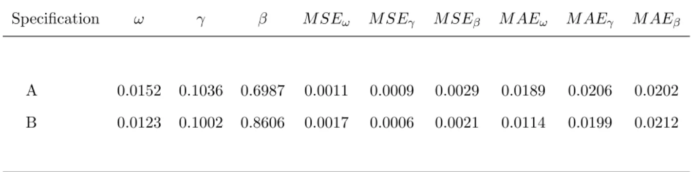
For the first simulation experiment the sample size is fixed atn= 1,000 and 2,000 synthetic samples are generated from specificationsA and B. Table 1.1 in Section 1.6 reports summary statistics for parameter estimates obtained from the MBP-SP algorithm under specifications A and B. The summary statistics include: the medians for the estimated parameters over their simulated distribution, the Monte Carlo mean absolute deviation, and the Monte Carlo mean squared error.7 Analyzing Table 1.1 in Section 1.6, we can conclude that the MBP-SP algorithm provides precise estimates of the conditional variance parameters and delivers similar results to those found in Christensen et al. (2012). The median number of iterations required to reach an estimator that converged, at least numerically, to the finite-sample fixed-point was five. The numerical tolerance for convergence was set to 1.0e−4 and the convergence criteria was chosen
7
to be|θˆn(k)−θˆn(k−1)|, where| · | is the Euclidean norm.
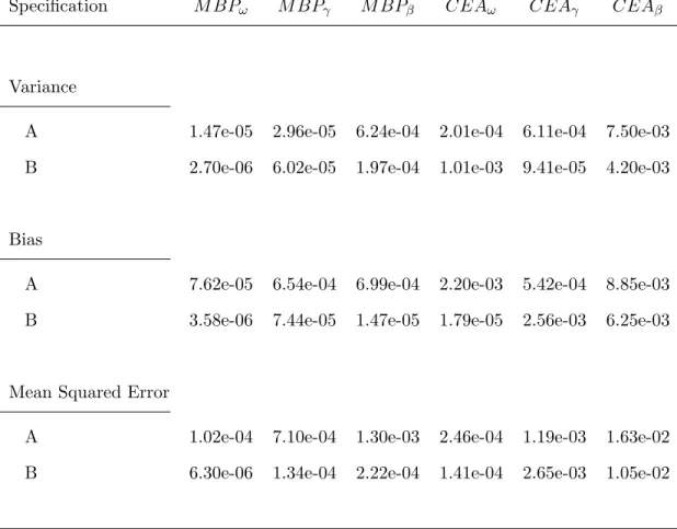
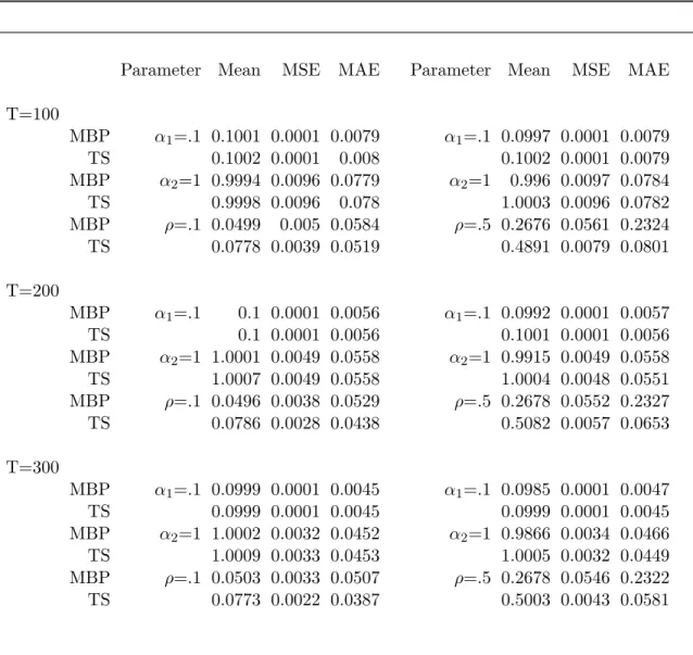
Recall that backfitting estimators can be inefficient since they neglect information contained within the log-likelihood function. Given this fact, and because the estimator proposed in Christensen et al. (2012) is in fact a backfitting estimator, we conduct a second simulation experiment to determine which estimation algorithm, the algorithm of Christensen et al. (2012) or the MBP-SP algorithm, yields more efficient estimators. We generate 2,000 synthetic samples of n = 3,000 observations from the data generating processes specified in the original Monte Carlo experiment. The parameters are estimated using the algorithm of Christensen et al. (2012) and the MBP-SP algorithm.
The Monte Carlo variance, bias and mean squared error are calculated over the 2,000 synthetic samples and are recorded in Table 1.2. The results suggest that the MBP-SP algorithm yields more efficient estimators than the algorithm of Christensen et al. (2012). In particular, the Monte Carlo variance and bias for the MBP-SP estimators are often an order of magnitude smaller than those obtained using the algorithm of Christensen et al. (2012). These results are in-line with earlier studies demonstrating that backfitting algorithms can yield inefficient and biased estimators.
1.3.2 Example Two: Predictability in the Merton Credit Risk Model
Credit risk models are used to describe the default process of firms and value corporate liabilities. Structural credit risk models provide an explicit relationship between the default-risk of a firm and the firm’s capital structure. In structural credit risk models firm default occurs if the market value of the firm at time-t, denoted by Yt∗, falls below some threshold representing its liabilities.
variable and implementation of the Merton model requires filtering Yt∗.
Denote the equity price of the firm at time-t, 0 ≤ t ≤τ, as Yt. Under the above capital structure Merton argued that the firm’s observable equity price Yt can be interpreted as the payoff of a European call option written on the firm’s unobservable market valueYt∗with strike price K and maturity date τ; that is, the firm’s equity price at the maturity date of it’s debt τ must be Yτ = max[Yτ∗−K,0]. The sequence of equity prices {Yt}nt=1 can then be seen as a
sequence of option prices written on the corresponding market values {Yt∗}n t=1.
Obtaining the option pricing relationship between Yt∗ and Yt requires specifying the firm’s market value dynamics. The Merton model assumes that the firm’s market value dynamics follow a geometric Brownian motion (GBM):
dYt∗
Yt∗ =µ·dt+σ·dW P
t , (1.13)
where µ is the drift coefficient, σ is the diffusion coefficient and WtP is a Brownian Motion under the historical probability measure P. Under the assumption that the risk-free interest rate r(r≥0) is deterministic risk-neutral valuation provides the key relationship between the firm’s equity priceYtand the latent market value Yt∗:
Yt=Yt∗Φ(dτ,t)−Kexp(−r(τ−t))Φ(dτ,t−σ√τ−t), (1.14)
where
dτ,t =
[ln(Yt∗/K) +
r+σ22
(τ −t)] σ√τ −t ,
τ −t is the time to maturity and Φ(·) is the cumulative distribution function of a standard normal random variable. That is, in the Merton model the firm’s observable equity value Yt is related to the firm’s latent market value Yt∗ through the Black and Scholes (1973) option pricing formula.
gτ,t(Yt, σ2).8 Given a value ofσ2 the firms unobservable market value Yt∗ can then be filtered using the relationshipYt∗ =gτ,t(Yt, σ2), where
Yt=g−τ,t1(Y ∗
t , σ2)≡Yt∗Φ(dτ,t)−Kexp(−r(τ −t))Φ(dτ,t−σ
√
τ −t).
The subscript τ in the function gτ,t(·, σ2) captures the dependence of the Black and Scholes formula on the time-to-maturity (τ−t).
Implementation of the Merton model requires estimating σ, µ and Yt∗ and can be carried out using the Maximum Likelihood approach described in Duan (1994, 2000). From equation (1.13), the log-likelihood function for the true latent returnsR∗t = log(Yt∗/Yt−∗1) is given by
L∗n(µ, σ) =−n
2 log(2πσ
2)−1
2 T X t=1
(R∗t −(µ−σ2
2 )) 2
σ2 −
T X t=1
log(Yt∗).
Using the option pricing relationshipYt∗=gτ,t(Yt, σ2), the Jacobian formula yields the observ-able log-likelihood function:
Ln(µ, σ) =−n
2log(2πσ
2)−1
2 T X t=1
(Rt(σ2)−(µ− σ
2
2 ))2
σ2 −
T X t=1
log(gτ,t(Yt, σ2))−
T X t=1
Φ log(dτ,t(σ2), (1.15)
whereRt(σ2) = log[gτ,t(Yt, σ2)/gτ,t−1(Yt−1, σ2)] are the implicit returns obtained from a specific
value of σ2 and (1.14), and
dτ,t(σ2) =
[ln(gτ,t(Yt, σ2)/K) +
r+σ22
(τ −t)]
σ√τ −t .
The last term in equation (1.15) corresponds to the Jacobian for the Black and Scholes formula and is needed to transition from the log-likelihood for the latent returns to the log-likelihood for the implicit returns Rt(σ2).
8
The Black and Scholes formula is strictly increasing inYt∗ for any plausible value of σ2 and so gτ,t(·, σ2)
Directly maximizing the log-likelihood in (1.15) yields parameter estimates forµ, σ2and esti-mates of the firm’s latent market values. However, this estimation procedure is computationally burdensome and can suffer from multiple local maxima. An alternative to direct maximiza-tion of the likelihood is the iterative estimamaximiza-tion approach known in the financial industry as the KMV (Kealhofer, McQuown and Vasicek) method. The KMV methods is implemented through the following steps: first, conditional on some initial estimate of σ2, the latent firm values are forecasted using (1.14); second, the forecasted firm values are used to update the parameter estimates by maximizing the observable log-likelihood, wheregτ,t(Yt, σ2) has been replaced by the forecasted value of Yt∗ obtained in the previous step. The estimation procedure is then iterated until convergence is achieved. The KMV method, while computationally simpler than Maximum Likelihood, is a backfitting estimation procedure in the spirit of Pastorello et al. (2003) and will not deliver the MLE upon convergence, see Fan et al. (2012) for a discussion.
A Semiparametric Merton Credit Risk Model
Maximum Likelihood estimation of the Merton credit risk model dominates other estimation methods, such as, the volatility-restriction approach and the pure proxy approach,9 in terms of bias and precision, so long as the model is correctly specified (Li and Wong, 2008). However, if the firm’s market value dynamics are not correctly specified the MLE will be biased and inconsistent, leading to poor estimates of σ2 and the latent firm values. In the Merton model
misspecification of the firm’s market value dynamics is particularly plausible since 1.13 implies that the firm’s market value returns are unpredictable. This assumption, which is true for many credit risk models besides the Merton model, stands in sharp contrast to a “substantial body of evidence that documents the predictability of financial asset returns,” Lo and Wang (1995). As discussed in Lo and Wang (1995), return predictability generally manifests itself in the drift of the process and has no affect on option prices since option prices are calculated under the risk neutral measure. Therefore, considering a more general specification for the drift coefficient in the firm’s market value dynamics will not alter the relationshipYt∗=gτ,t(Yt, σ2). Moreover,
9
allowing the firm’s market value dynamics to exhibit predictability would greatly enhance the applicability and robustness of the Merton model.
To incorporate predictability within the original Merton model we allow the drift coefficient in the diffusion model for the firm’s market value to be an arbitrary smooth function ofYt∗. The resulting semiparametric diffusion model for the firm’s market value dynamics is then given by
dYt∗ Yt∗ =η(Y
∗
t )·dt+σ·dWtP, (1.16)
where the drift coefficient η(·) is unknown and satisfies certain regularity conditions ensuring the existence of a solution to the stochastic differential equation (1.16).
Implementing this semiparametric version of the Merton model requires estimating Yt∗, σ and η(·). Maximum Likelihood estimation of Yt∗,σ and η(·) requires obtaining the transition density of this new diffusion model. Integrating the diffusion in (1.16) over the interval fromt tot+ ∆ we have
Z t+∆ t
dYu∗ Y∗
u =
Z t+∆ t
η(Yu∗)du+σ Z t+∆
t
dWuP =
Z t+∆ t
η(Yu∗)du+σ(WtP+∆−WtP). (1.17)
Furthermore, by Ito’s Lemma
Z t+∆ t
dYu∗ Y∗
u = ln
Y∗ t+∆
Yt∗
+σ
2
2 ∆. (1.18)
From (1.17) and (1.18) we obtain
ln Y∗
t+∆
Yt∗
= Z t+∆
t
η(Yu∗)du− σ 2
2 ∆ +σ(W P
t+∆−WtP), (1.19)
where for any t, (WtP+∆−WtP)∼N(0,∆) andN(a, b) a normal random variable with mean a and varianceb.
exactly integrated and the transition density can not be obtained in closed form for a fixed value of ∆. However, approximatingRtt+∆η(Yu∗)duby η(Yt∗)∆ yields the approximate model:
ln Y∗
t+∆
Yt∗
=
η(Yt∗)−σ 2
2
∆ +σ(WtP+∆−WtP). (1.20)
The only difference between equations (1.19) and (1.20) is the approximation due toRtt+∆η(Yu∗)du. Therefore, for sufficiently smooth η(·), the transition density derived from the model in equa-tion (1.20) and the transiequa-tion density of the diffusion model in equaequa-tion (1.16) should be very similar.
Using the approximated model
ln Y∗
t+∆
Yt∗
=
η(Yt∗)−σ 2
2
∆ +σ(WtP+∆−WtP),
where again we stress that the only actual approximation is due toη(Yt∗)∆, for ∆ = 1, we have
ln Y∗
t+1
Yt∗
Yt∗ ∼N
η(Yt∗)−σ 2
2
, σ2
. (1.21)
Equation (1.21) allows us to construct the conditional “latent” log-likelihood function for the diffusion model of the unobservable firm values. Similar to the fully parametric case, given the “latent” log-likelihood and the Black and Scholes formula, the Jacobian formula can be applied to obtain the observable conditional log-likelihood function:
Ln(σ2, η) =−n−1
2 ln(2πσ
2)− 1
2(n−1) n X t=1
[Rt(σ2)−(η(gτ,t(Yt, σ2))− σ22)]2 σ2
− 1
(n−1) n X
t=1
ln(gτ,t(Yt, σ2))− 1 n−1
n X
t=1
ln Φ(dτ,t(σ2)), (1.22)
where againRt(σ2) = ln(gτ,t(Yt, σ2)/gτ,t−1(Yt−1, σ2)) are the implicit returns obtained using a
specific value ofσ2and the Black and Scholes formula (1.14), anddτ,t(σ2) = [ln(gτ,t(Yt, σ2)/K)+ (r+σ2/2)(τ −t)]/σ√τ −t.
which can not be obtained without an estimator for σ2. Likewise, an estimator ofη(·) must be obtained before the conditional log-likelihood in (1.22) can be maximized to obtain an estimate of σ2.10 One idea is to obtain an estimate of η(·) at some preliminary estimate ofσ2 and plug this estimate into the conditional log-likelihood function (1.22). The resulting log-likelihood function can then be maximized with respect toσ2 and the process repeated until convergence
is achieved. However, from our earlier discussion of backfitting we know that such an estimation strategy may not adequately capture the information aboutσ2 contained in the drift function, potentially leading to biased and inefficient estimators.
Profile Estimation
The conditional log-likelihood in (1.22) depends on both finite and infinite dimensional param-eters and so a semiparametric estimation procedure is required to estimate σ2 and η(·). One potential means of estimating these quantities is profile likelihood. IfYt∗ were known we could estimateη(·) for a given value ofσ2 by maximizing, with respect toη, the smoothed likelihood function
n X j=1
[Rt(σ2)−(η−σ22)]2
σ2 K
Y∗ t −Yj∗
hn
, (1.23)
where K(·) is a bounded kernel function and hn is a bandwidth. It is simple to show that the maximizer of (1.23) is given by ˆη(Yt∗, σ2) =Pnj=1Rj(σ2)wj(Yt∗) +σ2/2, where
wj(Yt∗) =
KY ∗
t −Yj∗
hn
Pn
i=1K
Y∗
t−Yj∗
hn
.
Defining ¯Rt(σ2) =Pnj=1Rj(σ2)wj(Yt∗) we have ˆη(Yt∗, σ2) = ¯Rt(σ2) +σ2/2.
Unfortunately, calculatingη(Yt∗, σ2) at a fixed value ofσ2is not feasible since the firm value Yt∗ is unknown for fixedσ2. Even if such an estimator ofη(·) were feasible estimatingσ2 would
10Such an estimation procedure could be carried out simultaneously but this would require directly maximizing
require solving the following equation inσ2:
0 =σ4Mn(σ2) +σ2/2− 1 2(n−1)
n X
t=1
[Rt(σ2)−R¯t(σ2)]2, (1.24)
where
Mn(σ2) =M1,n(σ2) +M2,n(σ2) +M3,n(σ2), M1,n(σ2) =
1 2(n−1)σ2
n X
t=1
∂ ∂σ2[Rt(σ
2)−R¯
t(σ2)]2,
M2,n(σ2) =
1 (n−1)
n X
t=1
∂
∂σ2lngτ,t(Yt, σ 2),
M3,n(σ2) = 1 (n−1)
n X
t=1
∂
∂σ2ln Φ(dτ,t(σ 2)).
Solving equation (1.24) requires the use of inner and outer maximization loops and is compu-tationally complex.11
The MBP-SP algorithm could instead be used to iteratively solve 1.24 and obtain a com-putationally simpler estimate of σ2. In this setting the MBP-SP algorithm is implemented through the following steps.
Step (1): Provide an initial guess ˆσ2(1) and compute Yt∗(1) = gτ,t(Yt,σˆ2(1)) by inverting the Black and Scholes formula (1.14).
Step (2): For k ≥ 1, compute an estimate of the unknown function using {Yt∗(k)}n
t=1, ˆσ2(k)
and the updating rule:
ˆ
η(Yt∗(k),σˆ2(k)) = ¯Rt(ˆσ2(k)) + ˆσ2(k)/2. (1.25)
Step (3): Fork≥1, update the guess for ˆσ2(k) by solving
0 =σ4Mn(ˆσ2(k)) +σ2/2− 1 2(n−1)
n X
t=1
[Rt(ˆσ2(k))−R¯t(ˆσ2(k))]2. (1.26)
11
The updated guess ofσ2 can then be used to obtain{Yt∗(k+1)}n
t=1 by inverting the Black
and Scholes option pricing formula (1.14).
Step (4): Iterate between the updating rules (1.25) and (1.26) until convergence.
Equation (1.26) can be solved directly to yield a closed form solution for the updated guess of ˆσ2(k+1):
ˆ
σ2(k+1) = −
1 2 +
v u u t 1
4 + 2Mn(ˆσ
2(k)) 1
(n−1) n X t=1
[Rt(ˆσ2(k))−Rt(ˆ¯ σ2(k))]2
2Mn(ˆσ2(k)).
While estimation of σ2 using existing estimation methods would be computationally difficult, estimatingσ2using the MBP-SP algorithm only requires updating estimators using closed form solutions.
It is important to point out thatRt(σ2) is heterogeneous in a nonstationary manner because of the implicit returns dependence onτ. In principle the theory developed in Section 1.4 can not be readily applied to this setting without imposing additional regularity conditions. However, the simulation evidence given herein demonstrates that ignoring this issue does not have an impact on the resulting parameter estimates.12
Simulation Experiments
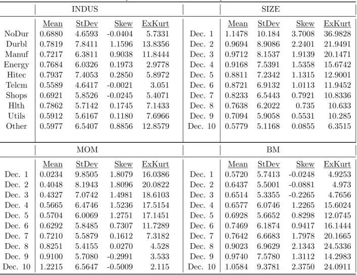
To illustrate the usefulness of the MBP-SP algorithm in the confines of the semiparametric credit risk model presented herein we devise and implement two Monte Carlo experiments. First, we construct 2,000 synthetic samples of 500 time series observations for daily returns, corresponding to two years of data on daily returns. The firms’ value trajectory is initialized at 104 and the face value of the firm’s debt is fixed at B = 900. The volatility parameter is fixed at σ2 =.09 and we consider two different specifications for the drift:
ηA(Yt∗)Yt∗=.01·Yt∗, ηB(Yt∗)Yt∗=.01·pYt∗.
12
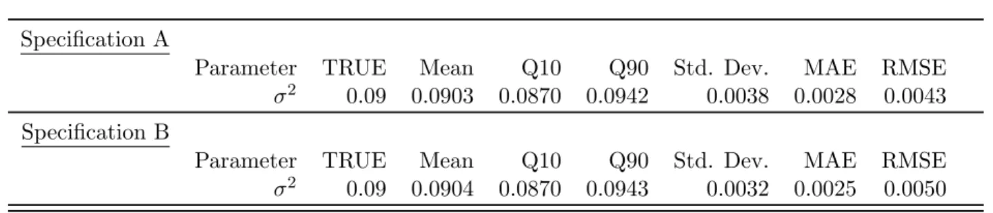
Under specificationAthe drift is constant and the process (Yt∗) is a geometric Brownian motion and under specification B the process (Yt∗) has a nonlinear drift. The parameter estimates are obtained by implementing the MBP-SP algorithm and a standard normal kernel is used in estimating the unknown drift function. The bandwidth for the procedure is chosen by leave-one-out cross-validation. For each specification we calculate the root mean squared error (RMSE), mean absolute error (MAE) and the Monte Carlo standard error for the estimated volatility parameter over the 2,000 replications. The median number of iterations required for the MBP-SP algorithm to achieve a convergent estimator under specification A was twenty-eight and under specificationB the algorithm needed thirty-two iterations to converge. The convergence criteria was specified as|ˆσ2(k)−σˆ2(k−1)|and the tolerance was set to 1.0e−04.
The results of the Monte Carlo experiment are contained in Table 1.3: Std. Dev. is the Monte Carlo standard deviation, MAE is the Monte Carlo mean absolute error and RMSE is the Monte Carlo root mean squared error. Generally speaking, Table 1.3 demonstrates that the MBP-SP algorithm yields precise estimates of the volatility parameterσ2, which was set to.09
for both specifications. This result is true across both specifications A and B.
The second Monte Carlo experiment attempts to determine what effect misspecification of the drift function has on the estimated volatility parameter. In particular, we construct the conditional log-likelihood function under the assumption that the drift in equation (1.16) is constant (η(Yt∗) =η), so (1.16) is a geometric Brownian motion and we are back in the original Merton model. However, for this Monte Carlo experiment the true drift function generating the data is specified as η(Yt∗) ·Yt∗ = .01 ·p
Yt∗ ( i.e., the data is actually generated from specificationB). Again we consider 2,000 synthetic samples of 500 time series observations for daily returns with the firm’s value trajectory initialized at 104 and the face value of the firm’s debt fixed at B = 900. The volatility parameter is also fixed at σ2 = .09. The parameter σ2 is estimated using a NR approach. The median number of iterations required to obtain a convergent estimator was thirteen.
much smaller mean absolute error and root mean squared error than the misspecified Maximum Likelihood estimator. Also, the mean parameter estimate obtained using the semiparametric method (.0904) is much closer to the true value (.0900) than the mean parameter estimate obtained from the misspecified Maximum Likelihood estimator (.0952) .
1.4
Asymptotic Properties
This section presents conditions under which the MBP-SP algorithm will converge and estab-lishes asymptotic properties for the corresponding estimators under consistent and inconsistent starting values. In this section we use high level assumptions, which can be verified for individual nonparametric estimation methods, to obtain asymptotic results for a general nonparametric estimator. In Section 1.8 we detail a set of more primitive conditions that guarantee satisfaction of these high level conditions if ˆη is obtained by kernel smoothing.
1.4.1 Consistency
This sub-section establishes consistency of ˆθ(nk) derived from the MBP-SP algorithm in Section 1.2.3. To establish asymptotic results for ˆθn(k) it is useful to re-parameterize the original score functionSn(θ), defined in Section 1.1, as Sn(θ, θ1), whereSn(θ, θ1) depends on the parameter θ through its own occurrence and the occurrence of θ1 treated as a nuisance parameter. For the MBP-SP algorithm the score function Sn(θ, θ1) is defined as:
Sn(θ, θ1) =n−1 n X
i=1
∂`i(θ,η(θˆ 1))
∂θ +
∂η(zˆ i, θ1) ∂θ
∂`i(θ1,η(θˆ 1))
∂η . (1.27)
To define the limit counterpart of Sn(θ, θ1) we require an assumption about the limiting behavior of ˆη(·, θ).
Assumption 1.
(i) supθ∈Θsupz∈Z|η(z, θ)ˆ −η(z, θ)|=op(1).
The limit score function S∞(θ, θ1) is given by
S∞(θ, θ1) =E
∂`(θ, η(θ1))
∂θ +
∂η(Z, θ1) ∂θ
∂`(θ1, η(θ1)) ∂η
. (1.28)
Define ˆθ(nk) as the argument maximizer of−|Sn(θ,θˆ( k−1)
n )|, where| · |is the Euclidean norm and define
¯
θn(ˆη(θ1)) = arg max θ
−|Sn(θ, θ1)|.
ˆ
θn(k) can then be represented equivalently as ˆθn(k) = ¯θn(ˆη(ˆθ
(k−1)
n )). Consistency of ˆθ(nk) for θ0 requires the following assumptions.
Assumption 2. There exist , b(Z), ˜b(Z), ˆb(Z) > 0 with E(b(Z)) < ∞, E(˜b(Z)) < ∞, E(ˆb(Z))<∞ such that
(i) for all θ∈Θ∂`(θ, η(θ))/∂θ is continuous atθ with probability one; (ii) supθ|∂`(θ, η(θ))/∂θ| ≤b(Z);
(iii) supθ|∂`(θ,η(θ))/∂θ˜ −∂`(θ, η(θ))/∂θ| ≤˜b(Z)(supθsupz|η(Z, θ)˜ −η(Z, θ)|);
(iv) `(θ, η)and∂`(θ, η)/∂θare Fr´echet differentiable inη. The Fr´echet derivative∂2`(θ, η)/∂θ∂η
satisfiessupθ,η|∂2`(θ, η)/∂θ∂η| ≤ˆb(Z).
Assumption 2 ensures that the limit score function S∞(θ, θ1) exists and satisfies
sup θ∈Θ
|Sn(θ, θ)−S∞(θ, θ)|=op(1).
The following assumption is required for identification of θ0.
Assumption 3.
(i) For any θ1 ∈Θ, the function θ7→ −|S∞(θ, θ1)| admits a unique maximizer θ[P¯ 0, η(θ1)], where P0 ∈ P is the true probability measure governing the observations;
(ii) The map θ[P¯ 0, η(·)] : Θ → Θ is continuous on Θ and θ[P¯ 0, η(·)] is continuous in η at
(ii) θ0 is a fixed-point of the map θ[P¯ 0, η(·)] .
The map ¯θ[P0, η(·)] can be interpreted as the limit of ¯θn(ˆη(·)) and θ0 = ¯θ[P0, η(θ0)] can be interpreted from the limit score equations S∞(θ0, θ0). Since the estimation problem is solved iteratively, consistency of ˆθ(nk) forθ0 requires an additional assumption about the uniqueness of this fixed point. To illustrate this consider the triangle inequality:
|θˆ(nk)−θ0| ≤ |θn(ˆ¯ η(ˆθ(nk)))−θ[P¯ 0, η(ˆθn(k))]|+|θ[P¯ 0, η(ˆθn(k))]−θ[P¯ 0, η(θ0)]|. (1.29)
Consistency of ˆθ(nk) forθ0 requires the right hand side (RHS) of equation (1.29) to converge to zero in probability as n → ∞. The first term on the RHS of (1.29) will converge to zero in probability if ¯θn(ˆη(θ1)) converges uniformly to ¯θ[P0, η(θ1)] in probability.
Lemma 1. Assume Θis a compact subset of the metric space ( ˜Θ,| · |). If Assumptions 1-3 are satisfied, then
sup θ1∈Θ
|θn(ˆ¯ η(θ1))−θ[P¯ 0, η(θ1)]| →0in probability.
By Lemma 1 consistency of ˆθ(nk) for θ0 depends on the second term on the RHS of (1.29). Consistent estimation ofθ0 will follow if either of the following scenarios are satisfied.
(i) If ˆθ(nk−1) is consistent for θ0 the second term on the RHS of (1.29) converges to zero by continuity of ¯θ[P0, η(·)]. Therefore, if the MBP-SP algorithm begins from a consistent estimator, ˆθ(nk) is consistent for θ0 at each k and the second term on the RHS of (1.29) converges to zero in probability.
(ii) If ˆθn(1) is not consistent for θ0, ¯θ[P0, η(·)] must be contracting over Θ and the number of iterations must go to infinity. The contraction mapping allows us to write
|θ[P¯ 0, η(ˆθn(k))]−θ[P¯ 0, η(θ0)]| ≤c|θˆ(nk)−θ0|
forc∈(0,1). Successive approximations then yield
Ask→ ∞the second term on the RHS of (1.29) converges to zero. Therefore, consistency of ˆθ(nk) forθ0 requires the following assumptions.
Assumption 4. The mapθ[P¯ 0, η(·)] : Θ→Θis contracting on Θ; i.e., there exists a c∈(0,1)
such that, for any θ1, θ2∈Θ
|θ[P¯ 0, η(θ1)]−θ[P¯ 0, η(θ2)]| ≤c|θ1−θ2|.
Assumption 5. θˆn(1) is a consistent estimator of θ0.
Proposition 1. Assume Θ is a compact subset of the metric space ( ˜Θ,| · |). Suppose Assump-tions 1-3 are satisfied, then
(i) under Assumption 4, θˆn(k) is consistent if k→ ∞ asn→ ∞;
(ii) under Assumption 5, θˆn(k) is consistent for any k= 1,2, ....
1.4.2 Information Dominance Condition
If ˆθ(1)n is not a consistent estimator of θ0 to achieve a consistent estimator ¯θ[P0, η(·)] must be contracting over Θ. While the contraction mapping condition may seem ad hoc this assumption is implied, at least locally, by an Information Dominance Condition (IDC). The equivalence between the IDC and the local contraction mapping condition was first noted by Song et al. (2005) and Fan et al. (2012) and requires that ¯θ[P0, η(·)] admit continuous partial derivatives. The IDC can be interpreted as a condition on the information contained in different portions of the Hessian. The IDC, and hence the local contraction mapping condition, will be satisfied if the information contained in the portion of the Hessian used to estimateθ0 is larger than the information contained in the portions of the Hessian that are ignored.
To detail the IDC recall that ¯θ[P0, η(θ1)] satisfies
Differentiating this expression with respect toθ1 we obtain
0 = ∂S∞(¯θ[P
0, η(θ1)], θ1)
∂θ
∂θ[P¯ 0, η(θ1)] ∂θ1 +
∂S∞(¯θ[P0, η(θ1)], θ1)
∂θ1 , (1.30)
where ∂S∞(·,·)
∂θ and
∂S∞(·,·)
∂θ1 are the partial derivatives of S∞(·,·) with respect to the first and
second arguments, respectively. Re-arranging 1.30, evaluating terms atθ0, and taking the norm yields
∂θ[P¯ 0, η(θ1)] ∂θ1
θ=θ0
=
−∂S∞(θ, θ 0)
∂θ θ=θ0
−1
∂S∞(θ0, θ1) ∂θ1
θ1=θ0
.
The IDC for the MBP-SP algorithm is then given by
−∂S∞(θ, θ 0)
∂θ θ=θ0
−1
∂S∞(θ0, θ1) ∂θ1
θ1=θ0
<1, (1.31)
where the derivatives in 1.31 are
∂S∞(θ, θ0) ∂θ
θ=θ0
=E
∂2`(θ, η0(Z, θ0)) ∂θ∂θ0
θ=θ0
, (1.32)
∂S∞(θ0, θ1) ∂θ1
θ1=θ0
=2E
∂η0(Z, θ1) ∂θ1
∂2`(θ0, η0(Z, θ1)) ∂η∂(θ1)0
θ1=θ0
+E
∂η0(Z, θ1) ∂θ1
∂2`(θ0, η0(Z, θ1)) ∂η∂η
∂η0(Z, θ1) ∂(θ1)0
θ1=θ0
+E
∂ `(θ1, η0(Z, θ1)) ∂η
∂2η0(Z, θ1) ∂θ1∂(θ1)0
θ1=θ0
. (1.33)
Obtaining reasonable estimates for θ0 requires, at a minimum, satisfaction of the IDC.