5873.pdf

(1)

BIFACTOR MODELS, EXPLAINED COMMON VARIANCE (ECV), AND THE USEFULNESS OF SCORES FROM UNIDIMENSIONAL

ITEM RESPONSE THEORY ANALYSES

Hally O’Connor Quinn

A thesis submitted to the faculty of the University of North Carolina at Chapel Hill in partial fulfillment of the requirements for the degree of Master of Arts

in the Department of Psychology.

Chapel Hill 2014

(2)

(3)

ABSTRACT

Hally O’Connor Quinn: Bifactor Models, Explained Common Variance (ECV), and the Usefulness of Scores from Unidimensional Item Response Theory Analyses

(Under the direction of David M. Thissen)

Item response data can be classified on a dimensionality continuum – which extends from theoretically unidimensional through essentially unidimensional to multidimensional. Data found to be essentially unidimensional are suitable for a UIRT model, whereas data evaluated to be too multidimensional are more appropriately modeled using MIRT. This investigation takes a theoretical, analytical approach to studying the relationship between a recently introduced index of dimensionality – estimated common variance (ECV) – and a criterion to determine the justifiability of reporting subscores – proportional reduction in mean squared error (PRMSE). Based on ECV values, recommendations are given for choosing

(4)

ACKNOWLEDGEMENTS

First and foremost, I would like to thank my advisor, Dave, for all of his kind words, support, patience, and brilliance. I have learned so much from him and would never have been able to finish this without his help.

I would also like to thank my other two committee members, Abigail and Patrick. Your questions, suggestions, and thoughts on my project helped clarify the way I communicate my research. Abigail, thank you for always being my cheerleader. Your encouragement has been invaluable.

I really appreciate the other professors who have helped me in various ways over the years - Bud, Antonio, Sy-Miin, Andrea Hussong, and Dan. They may not have had a hand in this particular project but their guidance, knowledge, and support made a big impression on me.

I would like to express sincere gratitude to current and past members of Dave's lab, especially Brooke, Yang, and Brian Stucky. Thank you for being awesome labmates and also genuinely great people.

Navigating graduate school thus far has been difficult for me but all of the current (and some alumni - Diane, Jolynn, and Ruth) members of the Thurstone Quant lab have made it possible. Some have paved the way ahead or beside me and shared their expertise, whereas others have been digging away in the trenches right there with me. We will always share this experience together and in a few years we might all agree that what does not kill you makes you stronger.

(5)

believed in me more than I believed in myself and ensured I did not give up.

(6)

TABLE OF CONTENTS

LIST OF TABLES ... viii

LIST OF FIGURES ... ix

CHAPTER 1. INTRODUCTION ... 1

Assumption of Unidimensionality ... 1

Measures of Dimensionality ... 3

Bifactor models ... 4

Explained common variance (ECV) ... 5

Where Do Bifactor Models Fit in with Other Multidimensional Models? ...7

Correlated simple structure models ...7

Second-order models ... 8

Testlet response models ... 9

Unidimensional models ... 11

Why the relationships among the models matter ... 11

Subscores and Proportional Reduction in Mean Squared Error (PRMSE) ... 12

CHAPTER 2. METHOD ... 15

Analytical Procedure ... 15

Data Structures ... 16

Evaluation of PRMSE Statistics ... 19

CHAPTER 3. RESULTS ... 20

CHAPTER 4. CONCLUSION AND DISCUSSION ... 30

(7)

APPENDIX B. PROPORTIONAL REDUCTION IN MEAN SQUARED

ERROR (PRMSE) ... 38

Calculation of ... 39

Calculation of ... 40

Example ... 41

Calculation of ... 41

Calculation of ... 44

Summary ... 45

(8)

LIST OF TABLES

TABLE 1 – Bifactor loading patterns ... 17 TABLE 2 – Bifactor model structures ... 17 TABLE 3 – Factor loading pattern 1: General dimension loadings = 0.50,

secondary dimension loadings = 0.50, ECV = 0.50 ... 20 TABLE 4 – Factor loading pattern 2: General dimension loadings = 0.70,

secondary dimension loadings = 0.50, ECV = 0.75 ... 23

TABLE 8 – Factor loading pattern 6: General dimension loadings = 0.70,

(9)

LIST OF FIGURES

FIGURE 1 – Bifactor model ... 5

FIGURE 2 – Dimensionality continuum ... 6

FIGURE 3 – Correlated simple structure model ... 8

FIGURE 4 – Second-order factor model ... 9

FIGURE 5 – Testlet response model (TRM)...10

FIGURE 6 – Unidimensional model ... 11

FIGURE 7 – Relation between ECV and PRMSE ratio for bifactor models with 3 secondary dimensions ... 28

FIGURE 8 – Relation between ECV and PRMSE ratio for bifactor models with 6 secondary dimensions ... 29

FIGURE 9 – Dimensionality continuum with suggestions on the use of ECV ... 31

(10)

CHAPTER 1. INTRODUCTION

Originally developed for ability and achievement testing in educational settings, item response theory (IRT) is increasingly being applied in psychological and health outcomes research as a method to create assessments, analyze items, and score questionnaires. IRT models can be useful when the measurement of an underlying latent variable (which can be a proficiency, an ability, an attitude, illness severity, or degree of symptomatology) is of interest. Latent trait estimates are based on models that take into account the properties of the items administered (item parameters) and an individual’s responses to those items. To calculate scores on a test or scale, the trace lines, or item response functions, are combined to form a likelihood that can be used to compute an estimate of an individual’s level of the latent variable (Thissen & Orlando, 2001; Thissen & Steinberg, 2009).

Assumption of Unidimensionality

(11)

p. 293). Consequently, it is useful to think of dimensionality as a continuum, which extends from theoretically unidimensional through essentially unidimensional to multidimensional item response data.

Until recently, IRT has been dominated by unidimensional IRT (UIRT). Over the past 15 years, there have been advances in estimation procedures for multidimensional IRT (MIRT; Edwards & Edelen, 2009; Reckase, 1997), which can model deviations from unidimensionality. Even with the development of MIRT models, the “appropriate” dimensionality assumption has to be satisfied; for that reason, it is necessary to assess dimensionality. Once assessed, data can be classified as essentially unidimensional and suitable for a UIRT model or if data are found to be too multidimensional, an MIRT model is likely more appropriate. Beyond the dimensionality found in data, researchers’ expectations and intensions for scores also factor into the use of UIRT or MIRT.

Health outcome researchers often want one score from a scale, which generally means breaking a questionnaire into multiple parts if there is departure from essential

unidimensionality. For example, some researchers have hypothesized that children cannot differentiate between anger, anxiety, and depressive symptoms and instead experience general negative-affect. A group of health outcome researchers conducted analyses to investigate dimensionality and discovered that children do indeed distinguish among the three emotions. The multidimensionality detected in the data led the researchers to create three separate scales instead of constructing one scale of emotional distress (Irwin et al., 2012; Irwin et al., 2010).

(12)

added value over the total score. In addition, the small number of items in each section often results in low subscore reliability.

Measures of Dimensionality

Many criteria have been proposed to evaluate dimensionality, such as the number of eigenvalues greater than 1.0 (Kaiser, 1960), the location of the “elbow” in a scree plot (Cattell, 1966), omega (McDonald, 1970; Heise & Bohrnstedt, 1970), DIMTEST (Stout, 1987), as well as countless others (Hattie, 1985). However, to date there is no single satisfactory statistical measure of unidimensionality. Often, several substandard indices are used to measure the dimensionality of a dataset but this can lead to conflicting assessments of the structure of the data.

This “gap” has created a carte blache of sorts in the applied literature, with researchers reporting subscores in addition to total scores when data are thought to be multidimensional. As noted previously, strictly unidimensional item response data are theoretical in nature and do not exist. Data determined to be essentially unidimensional are unidimensional enough to be characterized by a total score. The minor dimensions detectable in such data can be ignored and do not warrant the creation of subscales. Conversely, if data are too multidimensional to fit the definition of essential unidimensionality, the creation of subscales is necessary to accurately reflect variation from minor dimensions.

Historically another issue with the measurement of dimensionality is that unidimensionality has not been sufficiently differentiated from other concepts, such as homogeneity, reliability, and internal consistency. These terms are distinct and should not be used interchangeably, yet these words are often confused and an index of one concept may be falsely purported to be an index of unidimensionality (Hattie, 1985).

Therefore, the question of how researchers decide roughly where their item response data are located on the dimensionality continuum (unidimensional to essentially

(13)

simple way to decide whether a unidimensional or multidimensional IRT model should be fit to data? Should this decision incorporate information about whether subscores have added value over the total score? Is the choice between UIRT or MIRT affected by the usage of the scores? This investigation will attempt to answer these questions.

Bifactor models. As discussed previously, some item response data do not meet the assumption of unidimensionality, even when the criteria are expanded to include essential unidimensionality. This project focuses on the bifactor model and other related

multidimensional models as a way to model multidimensionality. In a bifactor model

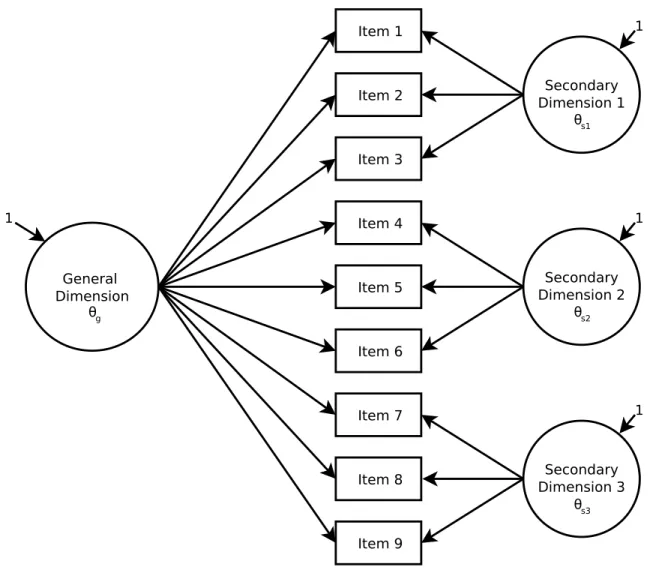
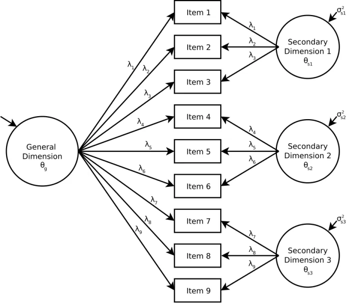
(sometimes referred to as a nested factors or hierarchical factor model), each item loads on one general latent dimension, as well as additional orthogonal secondary dimensions (see Figure 1; Gibbons & Hedeker, 1992). In Figure 1, all items load onto a secondary dimension but this is not necessary. If some items load onto only the general dimension, the model is classified as an incomplete bifactor model.

The general dimension is usually the main focus of the scale and accounts for the

commonality among all of the items. The secondary dimensions, which are specific to subsets of items, reflect item response covariation not explained by the general dimension. Typically, the general dimension is a broad construct (e.g., depressive symptoms, quality of life, or reading comprehension) and the secondary dimensions are restricted in scope to specific concepts (e.g., affective or somatic symptoms, disease worry or mobility, different reading passages).

In some ways, a bifactor model can be thought of as a helpful tool for measuring the dimensionality of scales. As the general and secondary dimensions are orthogonal (or

(14)

Figure 1. Bifactor model.

Explained common variance (ECV). Explained common variance (ECV; Bentler,

2009; Reise, Moore, & Haviland, 2010; Sijtsma, 2009; ten Berge & Sočan, 2004) is an indicator of unidimensionality. ECV is easily calculated using the estimated factor loadings of the general and secondary dimensions of a bifactor model:

(1)

Data that have a strong general factor compared to group factors will have high ECV. Exactly unidimensional (theoretical) data is the most extreme example of such data and has an ECV of 1.0. High values of ECV suggest data are unidimensional enough to be considered essentially

Item 1

Item 2

Item 3

Item 4

Item 5

Item 6

Item 7

Item 8

Item 9 General

Dimension

Secondary Dimension 1

Secondary Dimension 2

Secondary Dimension 3 1

1

1 θ_g

θ_s1

θ_s2

(15)

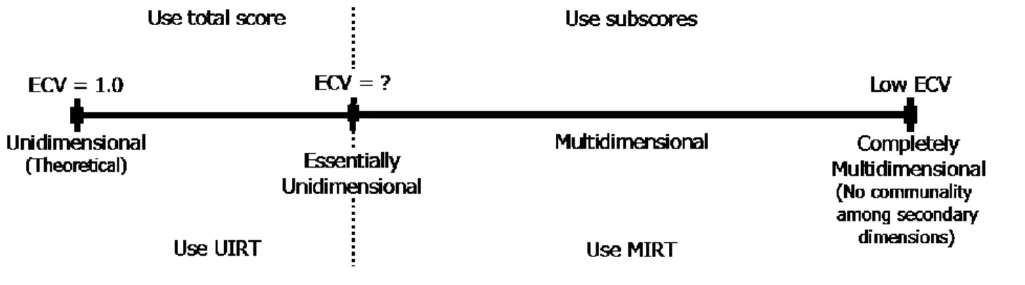
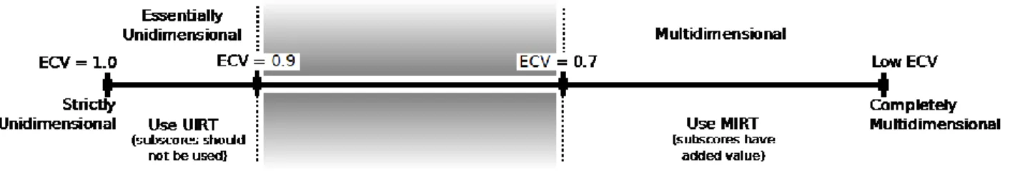
unidimensional and fit with a unidimensional model. Figure 2 illustrates how values of ECV correspond to the previously described dimensionality continuum.

Figure 2. Dimensionality continuum.

ECV is a helpful statistic because it represents the variance attributable to the general dimension out of the total common variance. Furthermore, ECV utilizes IRT and as a result, it is measuring unidimensionality in the latent variable space unlike the majority of other proposed unidimensionality indices. On the other hand, the equation for ECV makes it apparent that this is a model-based statistic, so it is dependent upon the correctness of the researcher’s

hypothesized bifactor model. It is currently unknown how these characteristics affect the utility of this unidimensionality index because too few studies have included the ECV statistic.

To the author’s knowledge, Reise and colleagues (Reise, 2012; Reise et al., 2010; Reise, Scheines, Widaman, & Haviland, 2013) are the only researchers to investigate the performance of ECV. In studies of strategies for building structural equation models, Reise (2012) found that:

“No benchmark values for ECV can be proposed for determining when the relative general factor strength is high enough so that it is safe to apply unidimensional models to multidimensional (bifactor) data because the relation between ECV and parameter bias is moderated by the structure of the data.” (p. 687)

(16)

This research will attempt to find benchmark ranges for the ECV statistic. It is not practical to try to locate a single ECV value that could be used as a cutoff for the choice between a unidimensional and multidimensional model, but it is likely possible to find a range of ECV where recommendations about model choice will be useful. To do this, we will use an IRT framework to answer the question, “At what values of ECV do subscores add value over and above information provided by the total score?” Prior experience with calculating ECV for various datasets suggests that data with an ECV below 0.70 are multidimensional and should be broken into multiple scales, whereas data with an ECV above 0.90 should be considered

essentially unidimensional.

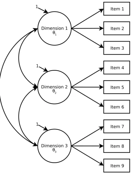
Where Do Bifactor Models Fit in with Other Multidimensional Models? Several multidimensional models are nested within the bifactor model structure. Ordered from least to most constrained, the models are: the bifactor model, the correlated simple structure model, and the second-order factor model, which is equivalent to the testlet response model. Researchers often compare the fit of nested models in order to decide which model fits the data appropriately. Usually the least restricted model is fit prior to any of the more restricted models of interest. As the bifactor model is the least constrained model in this sequence of multidimensional models, it is advisable to use it before any others and only continue with more constrained models if the bifactor model fits the data well.

(17)

Figure 3. Correlated simple structure model.

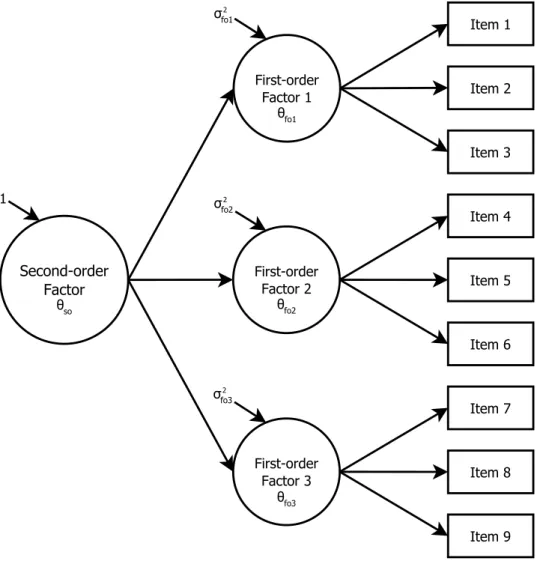
Second-order models. Second-order models (also called higher-order models) have a general dimension as well as specific dimensions. As shown in Figure 4, the difference between these models and bifactor models lies in the relations among these dimensions. Each item in this model loads onto a first-order factor (or specific dimension), which in turn, loads onto the second-order factor (or general dimension). Compared to Figure 3, second-order models account for the correlations among the dimensions in a correlated simple structure model (in this case, first-order factors) by putting a measurement structure on the correlations (the

second-order factor). It is also important to note that the relationship between the items and the second-order factor is indirect because the items only load onto the first-order factors.

Item 1

Item 2

Item 3

Item 4

Item 5

Item 6

Item 7

Item 8

Item 9 Dimension 1

Dimension 2

Dimension 3 1

1 1

θ₁

θ₂

(18)

With two subscales (or specific dimensions), a second-order factor model is an

equivalent yet different representation of a correlated simple structure model. A second-order factor model with three subscales may also have an exact relationship with a correlated simple structure model or may be merely close, depending on the particular structure of correlations among the subscales. When modeling four or more subscales, second-order factor models are no longer equivalent to correlated simple structure models; instead they are approximations of one another.

Figure 4. Second-order factor model.

Testlet response models.Like the models already described, the testlet response model (TRM) has one general dimension and multiple secondary dimensions (Wainer, Bradlow,

Item 1

Item 2

Item 3

Item 4

Item 5

Item 6

Item 7

Item 8

Item 9 First-order

Factor 1

First-order Factor 2

First-order Factor 3

Second-order Factor

1

θ_so

θ_fo1

θ_fo2

θ_fo3 σ_fo12

σ_fo22

(19)

& Wang, 2007). All items load onto the general dimension and only one of the secondary

dimensions. Both this description and the path diagram of the TRM, shown in Figure 5, are very similar to the bifactor model because the TRM is a restricted version of the bifactor model (Li, Bolt, & Fu, 2006). In a TRM, each item is constrained to have equal slopes (or loadings) on the general and secondary dimension with which it is associated, and the variances of the secondary dimensions are estimated, relative to the variance of the general dimension. Lastly, even though the path diagram of the second-order model (Figure 4) may not look like the TRM (Figure 5), they are formally equivalent (Rijmen, 2010; Yung, Thissen, & McLeod, 1999).

Figure 5. Testlet response model (TRM).

Item 1 Item 2 Item 3 Item 4 Item 5 Item 6 Item 7 Item 8 Item 9 General Dimension Secondary Dimension 1 Secondary Dimension 2 Secondary Dimension 3 1 θ_g θ_s1 θ_s2 θ_s3

σ_s12

σ_s22

σ_s32

(20)

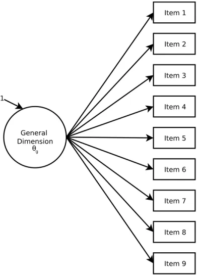
Unidimensional models. It is also possible to consider a unidimensional model as nested within the bifactor model. In a unidimensional model, each item loads onto the only general latent dimension in the model (Figure 6). If all of the loadings on the secondary dimensions in a bifactor model (Figure 1) are constrained to be zero, the model becomes a unidimensional model.

Figure 6. Unidimensional model.

Why the relationships among the models matter. Other than identifying the relationships among bifactor models, correlated simple structure models, second-order models, and TRMs, little use has been made of their interrelatedness thus far; however, this

investigation will utilize their connectedness. Using dimension-reduction techniques and maximum likelihood (ML) estimation, researchers have devised an efficient way to estimate the

Item 1

Item 2

Item 3

Item 4

Item 5

Item 6

Item 7

Item 8

Item 9 General

Dimension 1

(21)

parameters for bifactor models, even those with more than two or three “secondary” dimensions (Cai, 2010; Cai, Yang, & Hansen, 2011; Gibbons & Hedeker, 1992; Gibbons, Bock, Hedeker, Weiss, Segawa, Bhaumik, et al., 2007). Other computational algorithm and equipment advances for MIRT models have occurred as well, but computational issues for assessments with multiple subdomains continue. Therefore, calculating subscores using MIRT models continues to be difficult. Employing the relationships among models described previously to our advantage, it follows that bifactor models (with their efficient parameter estimation) have the potential to be a useful tool in the process of approximating parameters of highly dimensional correlated simple structure models. These parameters can subsequently be used to calculate IRT-scale subscores for the models (Thissen, 2012).

Subscores and Proportional Reduction in Mean Squared Error (PRMSE)

The decision to report subscores for an assessment is often made based on the goals of the researcher(s), mandated policies, and/or the belief that subscores yield more information than a single score. Although subscores have the potential to provide diagnostic information, researchers should only report subscores after they have demonstrated sufficient psychometric quality. The Standards for Educational and Psychological Testing indicate that it is acceptable to report more than one score from a test if the scores can be shown to be distinct from one another, as well as reliable, comparable, and valid (Standards 1.12 and 5.12; American Education Research Association [AERA], American Psychological Association [APA], & National Council on Measurement in Education [NCME], 1999). Subscores are widely reported in psychological and educational testing. Subscores are often found in the literature without any psychometric information to substantiate their quality, which suggests that the subscores do not meet the standards.

(22)

subscores. PRMSE was first applied in the context of classical test theory (Haberman, 2008), but its use has been extended to MIRT models (Haberman & Sinhary, 2010; Thissen, 2012). Using Haberman’s PRMSE criteria, many data sets were investigated in an attempt to determine when subscores have added value over total scores (Lyrén, 2009; Puhan, Sinharay, Haberman, & Larkin, 2010; Sinharay, 2010; Sinharay & Haberman, 2008). For the vast majority of tests examined, the subscores did not have added value. Some results revealed that it is possible for subscales in a test to be sufficiently distinct for subscores to provide meaningful diagnostic information. More broadly, researchers observed that subscores are more likely to provide added value when the total score has a low reliability, the subscore has a high reliability, and subscores are distinct from one another.

Tests reporting subscores need to use a statistical procedure (such as PRMSE) to demonstrate that the subscores have adequate psychometric quality, not merely state that they have added value over the total score (Haberman, 2008; Haberman & Sinhary, 2010; Reise, Bonifay, Haviland, 2013; Thissen, 2012). Subscores should not be “reported … or by extension, used in research or policy and decision-making” if they do not have added value over and above the total score (Reise et al., 2013, p. 136). In educational measurement, scores are almost always the main focus. This generally means that consumers want as many scores (and as much

(23)

(24)

CHAPTER 2. METHOD

This investigation takes a theoretical and analytical approach to studying the

relationship between ECV and PRMSE. We are particularly interested in attempting to make recommendations for choosing between UIRT and MIRT models based on ECV values. Also, we hope to offer suggestions about the appropriateness of reporting subscores, which is related to model choice, using ECV values.

Analytical Procedure

In order to study the relationship between ECV and PRMSE, we need to calculate the ECV and PRMSE for various bifactor models and the PRMSE for their corresponding correlated simple structure models. To do this, we utilize Thissen’s (2012) simplification of the generalized inverse Schmid-Leiman transformation (Yung et al., 1999) to convert parameters of

(25)

Once we have the parameters for the bifactor models and their corresponding correlated simple structure models, we calculate the bifactor model’s ECV and the PRMSE of two subscore estimates. The calculation of ECV is straightforward. The two subscore estimates that we are interested in are the expected a posteriori estimate for for subscale k computed from its

regression on from the second-order model [ ] and the expected a posteriori

estimate for for subscale k computed from a unidimensional IRT model fitted to subscale k

[ ]. Appendix B shows a simplified example of the calculation of both PRMSE

values used in the study.

Data Structures

This study crosses five data structures with eight factor loading patterns for a total of 40 conditions (5 structures times 8 factor loading patterns). In all conditions, the dimensions are orthogonal and the secondary dimensions are balanced (i.e., the secondary dimensions are made up of an equal number of items).

Table 1 shows the eight bifactor loading patterns that are investigated. The factor loading patterns were chosen such that the ECV is distinct for each pattern. In four of the factor loading patterns, each item loads onto both the general as well as a secondary dimension. The other four factor loading patterns are for incomplete bifactor models. In patterns 4, 6, 7, and 8, either one-third or two-one-thirds of the loadings from the secondary dimensions have been removed. In these patterns, some items load onto only the general dimension whereas others load onto both the general and a secondary dimension. Such structures occur in practice when item factor loadings on secondary dimensions are low.

(26)

investigation as it is unlikely that an assessment with 36 items and 12 group factors would be assumed to be unidimensional. All items are dichotomous.

Table 1

Bifactor loading patterns

Pattern ECV

Bifactor loadings Loadings removed from

General dimension

Secondary dimensions

of the secondary dimensions

1 0.50 0.6 0.6

2 0.66 0.7 0.5

3 0.69 0.6 0.4

4 0.75 0.7 0.5



5 0.80 0.8 0.4

6 0.85 0.7 0.5



7 0.86 0.8 0.4



8 0.92 0.8 0.4



Table 2

Bifactor model structures

Structure Total number of items

Number of secondary dimensions

Number of items per secondary dimension

1 9 3 3

2 18 3 6

3 18 6 3

4 36 3 12

(27)

The range of ECV values (0.50 to 0.92) for the factor loading patterns was chosen to be realistic for assessments used in practice. As ECV is based on model structure, it is theoretically possible to have an ECV lower than 0.50, but it is improbable to find such a structure with data analysis. An ECV higher than 0.92 is also possible, yet it is unlikely that such an assessment’s unidimensionality would be in question. The factor loadings were also selected to be

representative of assessments used in practice.

As noted previously, only a few studies have investigated ECV and none have looked at ECV with regard to scoring. “If a researcher has in mind an ‘essentially unidimensional’ but broadband trait measure, then high [percentage of uncontaminated correlations] PUC is desired in order to diminish the biasing effects of the group factors” (Reise, 2012, p. 688). In addition, Reise et al. (2013) found that “to the extent that PUC is high (>.80), the values of…[ECV] are less important in predicting bias. When PUC is lower than .80, researchers may consider ECV values greater than .60…as tentative benchmarks” (p. 18). In order to be able to compare the results of the present study, we also calculate PUC for each condition.

In a bifactor model, items that load onto a secondary dimension are correlated with other items that also load onto the same secondary dimension. Two sources of variance – from the general and secondary dimension – affect these correlations. When a unidimensional model is fit to such items, their estimated general factor loadings are biased because the model does not include the secondary dimensions. Items that belong to different secondary dimensions are correlated solely due to the general dimension; therefore, in a unidimensional model these correlations are not affected. To illustrate, in model structure 2, there are

unique correlations. There are correlations that are “contaminated” by

both general and secondary dimension variance. There are correlations that are

(28)

Evaluation of PRMSE Statistics

PRMSE values are not evaluated using a benchmark value, but instead by comparing them to other PRMSE values. The decision regarding the added value of subscores is made by comparing the two PRMSE values used in this study. Following the advice of Haberman, Sinharay, and Puhan (2009), if the reliability of the IRT subscore estimate computed using

information from the general dimension ( ) is greater than the reliability of the

IRT subscore estimate calculated from its own dimension ( ), subscores should not be reported because they offer no added value over total scores. In an effort to simplify decision-making about reporting subscores, as well as aid in visualizing the data, a PRMSE ratio was created of these two PRMSE values:

(2)

(29)

CHAPTER 3. RESULTS

Tables 3 through 6 show the results for the complete bifactor models, factor loading patterns 1, 2, 3, and 5, respectively. Tables 7 through 10 show the results for the incomplete bifactor model structures, factor loading patterns 4, 6, 7, and 8, respectively. All of these results are ordered by PRMSE ratio from smallest to largest. Each table includes the number of

secondary dimensions, number of items per secondary dimension, PUC, ECV, PRMSE ratio, as well as both PRMSE values that are used to calculate the ratio. Tables 7 through 10 also show

the PRMSE ratio, , and for the removed secondary dimension(s).

Table 3

Factor loading pattern 1: General dimension loadings = 0.50, secondary dimension loadings = 0.50, ECV = 0.50

Number of items per secondary

dimension PUC ECV PRMSE ratio

6 3 0.88 0.50 1.68 0.62 0.37

6 6 0.86 0.50 1.87 0.73 0.39

3 3 0.75 0.50 2.16 0.62 0.29

3 6 0.71 0.50 2.30 0.73 0.32

3 12 0.69 0.50 2.41 0.82 0.34

(30)

Table 4

6 3 0.88 0.66 1.17 0.62 0.53

6 6 0.86 0.66 1.30 0.73 0.56

3 3 0.75 0.66 1.39 0.62 0.45

3 6 0.71 0.66 1.50 0.73 0.49

3 12 0.69 0.66 1.58 0.81 0.51

Note: PUC = percentage of uncontaminated correlations; ECV = explained common variance; PRMSE = proportional reduction in mean squared error; PRMSE ratio = ; = estimate of the true subscore for subscale k; = estimate of the true total score from the general dimension of the second-order model; = estimate of the true subscore for subscale k computed from a unidimensional IRT model fitted to subscale k.

Table 5

6 3 0.88 0.69 1.03 0.56 0.55

6 6 0.86 0.69 1.20 0.71 0.59

3 3 0.75 0.69 1.24 0.56 0.45

3 6 0.71 0.69 1.38 0.71 0.51

3 12 0.69 0.69 1.48 0.82 0.55

(31)

Table 6

Factor loading pattern 5: General dimension loadings = 0.80, Secondary dimension loadings = 0.40, ECV = 0.80

6 3 0.88 0.80 0.93 0.61 0.66

6 6 0.86 0.80 1.03 0.72 0.70

3 3 0.75 0.80 1.06 0.62 0.58

3 6 0.71 0.80 1.13 0.71 0.63

3 12 0.69 0.80 1.19 0.79 0.66

Note: PUC = percentage of uncontaminated correlations; ECV = explained common variance; PRMSE = proportional reduction in mean squared error; PRMSE ratio = ; = estimate of the true subscore for subscale k; = estimate of the true total score from the general dimension of the second-order model; = estimate of the true subscore for subscale k computed from a unidimensional IRT model fitted to subscale k.

As the tables show, there are three possible ways to decrease PUC: 1) decrease the number of secondary dimensions in a test without removing items from the test (which means increasing the number of items per secondary dimension), 2) increase the number of items per secondary dimension without adding items to the test (which results in decreasing the number of secondary dimensions), or 3) increase the number of items per secondary dimension by lengthening the test. Therefore, many small secondary dimensions produce a test with a high PUC value, whereas a test with fewer secondary dimensions that are large will have a lower PUC value. On the other hand, test length, number of secondary dimensions, and number of items per secondary dimension do not affect ECV.

Based on Tables 3 through 6, the PRMSE ratio appears to be related to the PUC. As PUC decreases, the ratio increases. The numerator, , increases as items are added to

(32)

23

Table 7

Factor loading pattern 4: General dimension loadings = 0.70, secondary dimension loadings = 0.50, ECV = 0.75

dimension _PUC _ECV

PRMSE ratio

Removed secondary dimension(s)

Mean PRMSE

ratio PRMSE

Ratio

6 3 0.92 0.75 1.13 0.62 0.55 0.66 0.55 0.83 0.90

6 6 0.90 0.75 1.25 0.73 0.59 0.79 0.70 0.88 1.02

3 3 0.83 0.75 1.31 0.62 0.47 0.77 0.55 0.71 1.04

3 6 0.80 0.75 1.37 0.73 0.53 0.87 0.70 0.80 1.12

3 12 0.79 0.75 1.41 0.81 0.57 0.93 0.81 0.87 1.17

Note: PUC = percentage of uncontaminated correlations; ECV = explained common variance; PRMSE = proportional reduction in mean squared error; PRMSE ratio = ; = estimate of the true subscore for subscale k; = estimate of the true total score from the general dimension of the second-order model; = estimate of the true subscore for subscale k

(33)

24

Table 8

dimension _PUC _ECV

PRMSE ratio

Mean PRMSE

ratio PRMSE

Ratio

6 3 0.96 0.85 1.11 0.62 0.56 0.65 0.55 0.85 0.88

6 6 0.95 0.85 1.22 0.73 0.60 0.77 0.70 0.91 0.99

3 3 0.92 0.85 1.26 0.62 0.49 0.74 0.55 0.74 1.00

3 6 0.90 0.85 1.31 0.73 0.55 0.83 0.70 0.84 1.07

3 12 0.90 0.85 1.36 0.81 0.60 0.90 0.81 0.90 1.13

(34)

25

Table 9

dimension _PUC _ECV

PRMSE ratio

Mean PRMSE

ratio PRMSE

Ratio

6 3 0.92 0.86 0.91 0.61 0.68 0.72 0.61 0.85 0.81

6 6 0.90 0.86 1.00 0.72 0.72 0.81 0.73 0.90 0.91

3 3 0.83 0.86 1.02 0.62 0.60 0.80 0.61 0.75 0.91

3 6 0.80 0.86 1.08 0.71 0.66 0.88 0.73 0.83 0.98

3 12 0.79 0.86 1.12 0.79 0.71 0.93 0.82 0.88 1.03

(35)

26

Table 10

dimension _PUC _ECV

PRMSE ratio

Mean PRMSE

ratio PRMSE

Ratio

6 3 0.96 0.92 0.89 0.61 0.69 0.71 0.61 0.86 0.80

6 6 0.95 0.92 0.98 0.72 0.73 0.80 0.73 0.91 0.89

3 3 0.92 0.92 1.00 0.62 0.62 0.78 0.61 0.77 0.89

3 6 0.90 0.92 1.05 0.71 0.68 0.86 0.73 0.85 0.95

3 12 0.90 0.92 1.09 0.79 0.72 0.91 0.82 0.90 1.00

(36)

the remains approximately the same when additional secondary dimensions are

added to a test but the number of items per secondary dimension remains constant. Lastly, the decreases when test length is held constant, but secondary dimensions are added,

which results in a decrease in the number of items per secondary dimension. The denominator,

, increases as the number of secondary dimensions increases (without adding

additional items to the test) or as the number of items per secondary dimension increases (without adding additional secondary dimensions). Clearly, the number of items per secondary dimension largely influences , whereas the number of secondary dimensions and

the length of a test affect . Tables 7 through 10 illustrate that as PUC decreases,

the PRMSE ratio for the removed secondary dimension loadings as well as the mean PRMSE ratio of the incomplete bifactor models increases.

Figures 7 and 8 show the relation between ECV and PRMSE ratio for the bifactor models with 3 and 6 secondary dimensions, respectively. Based on the figures and the previous

observations about PUC and PRMSE, we notice that holding ECV constant, the PRMSE ratio increases with the addition of items to the test (while keeping the number of secondary

dimensions constant, hence adding items to each secondary dimension), as the test gets shorter from the removal of secondary dimensions, or as the number of secondary dimensions decrease (while the test length is kept constant). Looking at the figures and across tables 3 through 10, each of which shows only one factor loading pattern or ECV, it appears as though there is a range of possible PRMSE ratios for any particular ECV value. When ECV is low, the range of PRMSE ratios is large, but as ECV increases the range decreases. Furthermore, as ECV increases, the value of the PRMSE ratio decreases generally speaking.

(37)

ratio lower than 1.0. Five of the 20 incomplete bifactor models have a PRMSE value equal to or lower than 1.0 and 13 have a mean PRMSE ratio equal to or lower than 1.0. Thus, for most of the bifactor model structures investigated in the present study, subscores will have added value over a total score based on PRMSE values.

Figure 7. Relation between ECV and PRMSE ratio for bifactor models with 3 secondary

dimensions.

0.6 0.8 1.0 1.2 1.4 1.6 1.8 2.0 2.2 2.4 2.6

0.5 0.6 0.7 0.8 0.9 1.0

ECV

P

R

M

S

E

ra

ti

o

Number of Items

3 items

6 items

12 items

Model Structures

Complete bifactor

1/3 loadings removed

2/3 loadings removed

(38)

Figure 8. Relation between ECV and PRMSE ratio for bifactor models with 6 secondary dimensions.

.

0.6 0.8 1.0 1.2 1.4 1.6 1.8 2.0 2.2 2.4 2.6

0.5 0.6 0.7 0.8 0.9 1.0

ECV

P

R

M

S

E

ra

ti

o

Number of Items

3 items 6 items

Model Structures

(39)

CHAPTER 4. CONCLUSION AND DISCUSSION

This is the first investigation of the relationship between ECV and PRMSE. Once a bifactor model has been fit to data, the calculation of ECV is simple and quick. On the other hand, PRMSE is much more difficult and time consuming to compute. With the added information from this study, it is no longer necessary to take the time and energy to calculate PRMSE for every scale. Based solely on ECV, we now have appropriate knowledge to be able to make certain decisions about models and scores.

We can easily compute ECV if a bifactor model can be fit to data and it fits well. What does ECV suggest about the dimensionality of data, as it applies to the use of UIRT or MIRT?

If ECV is greater than 0.90, we conclude that the data are unidimensional enough to

use UIRT. We can also say that the PRMSE ratio (as used in the present study) is less than or approximately equal to 1.0.

If ECV is between 0.70 and 0.90, we advise using additional information to choose a

model. This is a grey area on the dimensionality spectrum (see Figure 9); therefore, using ECV alone is not adequate here. We advise calculating PRMSE and taking into account the usage of the proposed subscores.



If ECV is less than 0.70, there is enough multidimensionality in the data to warrant

modeling it with MIRT. Subscores for the multiple subscales will provide added value over simply reporting a total score.

This project aimed to further research on the dimensionality statistic, ECV. Although we did not find a single ECV value that gives a clear-cut answer to how multidimensional is too

(40)

Figure 9. Dimensionality continuum with suggestions on the use of ECV.

exploration provided information about ECV and its relation with PRMSE, there were

limitations. Future research will need to incorporate simulations and use actual data to explore our conclusions. Also, we only considered dichotomous items; therefore, polytomous items should be used in subsequent studies.

(41)

APPENDIX A. SIMPLIFICATION OF THE GENERALIZED INVERSE SCHMID-LEIMAN TRANSFORMATION

The generalized inverse Schmid-Leiman transformation is an algorithm provided by Yung et al. (1999) that converts parameters of an unconstrained bifactor model to parameters of a second-order factor model. If a bifactor model can be converted into a TRM by imposing equality constraints, this algorithm can be simplified, as shown by Thissen (2012). Thissen’s (2012) shortcut goes a step further and converts the TRM parameters into those of a correlated simple structure model. This process is illustrated using the following bifactor model (condition 3 – structure 1, factor loading pattern 3):

,

In order for this loading matrix to conform to the equality constraints of the TRM (each item has equal loadings on the general and secondary dimension with which it is associated), it is

necessary for the factor loading matrix to be:

(42)

To solve for , the variances of the secondary dimensions in the TRM, the following sets of

simultaneous equations are solved:

(3)

Here, , , and represent the variances of the secondary dimensions in the TRM. Note

that in the TRM, the variances of the secondary dimensions are estimated (or in this case simply calculated) relative to the general dimension; hence the general dimension variance of 1.0. The variance of the first secondary dimension is:

(4)

The same calculation is carried out for the remaining variances of the secondary dimensions in the TRM:

This results in , the variances of the general and secondary dimensions in the TRM:

(43)

Using the variances of the secondary dimensions from the TRM, the second-order factor loadings for the second-order factor model ( , , and ) are calculated:

(5)

To calculate the random variance components of the first-order factors for the second-order factor model, we use:

(44)

To calculate the factor loadings for the correlated simple structure model, we use the secondary dimension factor loadings from the TRM and the matrix Y (Thissen, 2012). Y is a simplified version of a matrix from the generalized inverse Schmid-Leiman transformation (Yung et al., 1999).

(7)

Y is then used with the secondary dimension factor loadings from the TRM to calculate the factor loadings for the correlated simple structure model:

(45)

Using the second-order factor loadings from the second-order factor model, the correlation matrix among the factors of the correlated simple structure model is calculated:

(9))

(46)

37

Figure 10. Generalized inverse Schmid-Leiman transformation (from unconstrained bifactor to correlated simple structure model).

(47)

APPENDIX B. PROPORTIONAL REDUCTION IN MEAN SQUARED ERROR (PRMSE)

Haberman and colleagues (Haberman, 2008; Haberman & Sinharay, 2010) advocate the use of the proportional reduction in mean squared error (PRMSE) to evaluate the precision of subscore estimates in an attempt to avoid reporting subscores which do not provide useful information. PRMSEs range from 0 to 1, with larger values indicating more accurate estimates (because a large PRMSE corresponds to a smaller mean squared error). PRMSE and reliability are conceptually related criteria, which is evident when looking at the general form of PRMSE,

. (10)

Haberman (2008) introduced PRMSE based on classical test theory and the concept of true scores. Using this approach, PRMSEs are used to evaluate the quality of three true subscore approximations based on the observed subscore, the observed total score, and a combination of the observed subscore and the observed total score. This paper refers to the PRMSEs as

, , and , respectively. Haberman et al. (2009) recommend that if

is greater than , subscores should not be reported because they do not offer

“added value over the total scores” (p. 81). In addition, the use of the weighted average is suggested only if is markedly larger than and because the weighted

average involves slightly more computation, and score augmentation, as it is called, can be somewhat difficult to explain to consumers. Haberman and Sinharay (2010) extended their work with PRMSE to MIRT models. They suggest choosing between the two based on model preference (classical test theory or MIRT).

This study uses parameter estimates from bifactor as well as correlated simple structure models to compute subscore estimates. The subscore estimates from both models are then compared using PRMSE in an attempt to determine if subscores should be reported. The two

estimates of subscores that we are interested in are the expected a posteriori estimate for for

(48)

and the expected a posteriori estimate for for subscale k computed from a unidimensional IRT

model fitted to subscale k [ ].

Calculation of

To calculate , we carry out steps 1-5 for each quadrature point in space.

49 quadrature points (at θ values -6.0 to 6.0 by 0.25 standard deviation units) are used for the 4-dimensional models (bifactor model structures 1, 2, and 4). The number of quadrature points is reduced to 9 (at θ values -4.0 to 4.0 by 1.0 standard deviation units) for the 7-dimensional models (bifactor model structures 3 and 5) due to computational time.

1) Using the parameters from the unconstrained bifactor model, we calculate the trace surface for item i using the multidimensional two-parameter logistic (M2PL) model:

(11)

T is the surface in k-dimensional space that traces the probability of a positive

response ( ) for item i. is a k-dimensional vector of the slope parameters, is a k

-dimensional vector of scores on the latent variables, and is the intercept parameter (a

scalar value).

2) The information computation begins with the identity matrix (that is the inverse of the covariance matrix for the population distribution and has the same number of

dimensions as the model). Item i’s information calculated at each point is added. This calculation uses item i’s vector of slope parameters and the probability of endorsement for item i evaluated at a specific point:

(12) 3) After information is calculated for item i, the trace surface is computed for the next item

at the same point in space. The trace surface value is used in the information

(49)

trace surface and information are subsequently calculated for the remainder of the items and added to the total information matrix.

4) The error covariance matrix for the point in space is then found by taking the inverse of the information matrix:

₍₁₃₎

5) To find the weighted error variance for the general factor, the error variance

corresponding to the general factor (the element in the first column of the first row in the error covariance matrix; ) is weighted at each by the standard normal Gaussian

population density:

(14)

Steps 1-5 are carried out for the remainder of the quadrature points. The weighted error variances are summed to create an error variance for the general factor for the entire test.

6) To calculate the reliability estimate of the general factor of the bifactor model, the average error variance for the model is subtracted from one:

(15)

7) Last, subscale k’s PRMSE based on the general factor is found by multiplying the general factor’s reliability estimate with the subscale k’s second-order factor loading from the second-order model:

(16)

Calculation of

To calculate , we follow the same general steps described above. The main

differences in this PRMSE calculation are that the model parameters are from simple structure models and therefore, we are working in unidimensional space. Appendix A explains the

(50)

correlated simple structure models. Instead of the M2PL model, we use a unidimensional 2PL IRT model for subscale k:

(17)

Example

In order to illustrate the calculation of the two PRMSE values used in the study, a simplified example with only three dimensions is used (which is not one of the study conditions). Below is the M2PL bifactor structure used as the example:

,

For illustrative purposes, I use 3 quadrature points at θ values -1.0 to 1.0 by 1.0 standard deviation units.

Calculation of . For the first quadrature point (-1, -1, -1), the first item’s trace surface is computed:

(18)

The information calculation begins with the identity matrix.

(51)

Information is then calculated for the first item: (19)

and added to the information matrix above:

The trace surface and information matrices are then computed for the remainder of the items at the first quadrature point (-1, -1, -1).

, , , , ,

The information matrices are added together to form the information matrix for the test at the first quadrature point.

(52)

Next the error covariance matrix is computed:

(20)

The weighted error variance is found by weighting the error variance that corresponds to the general factor at each by the standard normal Gaussian population density:

(21)

The error variance is computed in the same way for the remaining 26 quadrature points and then all 27 values are added together to compute the average error variance for the test.

The reliability estimate for the general factor is:

(22)

Using this reliability estimate, we are able to find the first subscale’s PRMSE estimate from its regression on the second-order factor (from the second-order factor model):

(53)

Calculation of . After using the methods described in Appendix A to calculate the item parameters for the corresponding simple-structure model, the first item’s trace line is calculated for the first quadrature point (-1):

(24)

The information calculation begins with 1.0 because the information that is attributed to the population distribution is 1.0 across (from the assumption that the population distribution is standard normal Gaussian).

Information is then calculated for the first item:

(25)

and added to the information value above.

The trace lines and information are then computed at the same quadrature point (-1) for the other two items that make up the first subscale.

,

The information values are then added together to form the information for the subscale at the quadrature point.

Next the error variance is computed:

(54)

The weighted error variance is found by multiplying the error variance by the standard normal Gaussian population density:

(27)

The average error variance is computed in the same way for the remaining 2 quadrature points and then all 3 values are added together to compute the average error variance for the subscale.

,

The marginal reliability estimate for this subscale is:

(28)

Summary

(55)

REFERENCES

American Educational Research Association (AERA), American Psychological Association (APA), & National Council on Measurement in Education (NCME). (1999). Standards

for educational and psychological testing. Washington, DC: AERA.

Bentler, P. M. (2009). Alpha, dimension-free, and model-based internal consistency reliability.

Psychometrika, 74, 137–143.

Cai, L. (2010). A two-tier full-information item factor analysis model with applications.

Psychometrika, 75, 581-612.

Cai, L., Yang, J., & Hansen, M. (2011). Generalized full-information item bifactor analysis.

Psychological Methods, 16, 221-248.

Cattell, R. B. (1966). The scree test for the number of factors. Multivariate Behavioral Research, 1, 245-276.

Edwards, M.C. & Edelen, M. O. (2009). Special topics in item response theory. In R. Millsap & A. Maydeu-Olivares, The sage handbook of quantitative methods in psychology. London: Sage Publications.

Embretson, S. E. & Reise, S. (2000). Item response theory for psychologists. Mahwah, NJ: Erlbaum Publishers.

Gibbons, R., Bock, R., Hedeker, D., Weiss, D., Segawa, E., Bhaumik, D., et al. (2007). Full-information item bifactor analysis of graded response data. Applied Psychological

Measurement, 31, 4-19.

Gibbons, R. D., & Hedeker, D. R. (1992). Full-information item bi-factor analysis.

Psychometrika, 57, 3, 423-436.

Haberman, S. J. (2008).When can subscores have value? Journal of Educational and

Behavioral Statistics, 33, 204–229.

Haberman, S.J., Sinharay, S., & Puhan, G. (2009). Reporting subscores for institutions. British

Journal of Mathematical and Statistical Psychology, 62, 79–95.

Hattie, J. (1984). An empirical study of various indices for determining unidimensionality.

Multivariate Behavioral Research, 19, 49-78.

Hattie, J. (1985). Methodology review: Assessing unidimensionality of tests and items. Applied

(56)

Heise, D. R., & Bohrnstedt, G. W. (1970). Validity, invalidity, and reliability. In E. F. Borgatta & G. W. Bohrnstedt (Eds.), Sociological methodology (pp. 104-129). San Francisco CA: Jossey-Bass.

Irwin, D.E., Stucky, B.D., Langer, M.M., Thissen, D., DeWitt, E.M., Lai, J-S, Yeatts, K.B., Varni, J.W., and DeWalt, D.A. (2012). PROMIS Pediatric Anger Scale: An item response theory analysis. Quality of Life Research, 21, 697-706.

Irwin, D., Stucky, B.D., Thissen, D., DeWitt, E.M., Lai, J.S., Yeatts, K., Varni, J., & DeWalt, D.A. (2010). An item response analysis of the Pediatric PROMIS Anxiety and Depressive Symptoms Scales. Quality of Life Research, 19, 595-607.

Kaiser, H.F. (1960). The application of electronic computers to factor analysis. Educational and

Psychological Measurement, 20, 141-151.

Li, Y., Bolt, D. M., & Fu, J. (2006). A comparison of alternative models for testlets. Applied

Psychological Measurement, 30, 3–21.

Luecht, R. M., Gierl, M. J., Tan, X., & Huff, K. (2006, April). Scalability and the development of useful diagnostic scales. Paper presented at the annual Meeting of the National Council on Measurement in Education, San Francisco, CA.

Lyrén, P. (2009). Reporting subscores from college admission tests. Practical Assessment,

Research, and Evaluation, 14, 1–10.

McDonald, R. P. (1970). The theoretical foundations of principal factor analysis, canonical factor analysis, and alpha factor analysis. British Journal of Mathematical and Statistical

Psychology, 23, 1-21.

Puhan, G., Sinharay, S., Haberman, S. J., & Larkin, K. (2010). The utility of augmented

subscores in a licensure exam: An evaluation of methods using empirical data. Applied

Measurement in Education, 23, 266-285.

Reise, S. P. (2012). The rediscovery of bifactor measurement models. Multivariate Behavioral

Research, 47, 667-696.

Reise, S. P., Bonifay, W. E., & Haviland, M. G. (2013). Scoring and modeling psychological measures in the presence of multidimensionality. Journal of Personality Assessment,

95, 129-140.

Reise, S. P., Moore, T. M., & Haviland, M. G. (2010). Bifactor models and rotations: exploring the extent to which multidimensional data yield univocal scale scores. Journal of

(57)

Reise, S. P., Moore, T. M., & Maydeu-Olivares, A. (2011). Targeted bifactor rotations and assessing the impact of model violations on the parameters of unidimensional and bifactor models. Educational and Psychological Measurement, 71, 684–711.

Reise, S. P., Scheines, R., Widaman, K. F, & Haviland, M. G. (2013). Multidimensionality and structural coefficient bias in structural equation modeling: A bifactor

perspective. Educational and Psychological Measurement, 73, 5-26.

Rijmen, F. (2010). Formal relations and an empirical comparison between the bi-factor, the testlet, and a second-order multidimensional IRT model. Journal of Educational

Measurement, 47, 361-372.

Rindskopf, D., & Rose, T. (1988). Some theory and applications of confirmatory second-order factor analysis. Multivariate Behavioral Research, 23, 51–67.

Sijtsma, K. (2009). On the use, the misuse, and the very limited usefulness of Cronbach’s alpha.

Psychometrika, 74, 107–120.

Sinharay, S. (2010). How often do subscores have added value? Results from operational and simulated data. Journal of Educational Measurement, 47, 150–174.

Sinharay, S., & Haberman, S. J. (2008). Reporting subscores: A survey (ETS Research Memorandum RM-08-18). Princeton, NJ: Educational Testing Service.

Stout, W. (1987). A nonparametric approach for assessing latent trait dimensionality.

Psychometrika, 52, 589-618.

Stout, W. (1990), A new item response theory modeling approach with applications to unidimensionality assessment and ability estimation. Psychometrika, 55, 293-325.

ten Berge, J. M. F., & Sočan, G. (2004). The greatest lower bound to the reliability of a test and the hypothesis of unidimensionality. Psychometrika, 69, 613–625.

Thissen, D. (2012, July). Using the testlet response model as a shortcut to multidimensional

item response theory subscore computation. Paper presented at the 77th Annual

Meeting of the Psychometric Society, Lincoln, NE.

Thissen, D., & Orlando, M. (2001). Item response theory for items scored in two categories. In D. Thissen & H. Wainer (Eds), Test Scoring. Hillsdale, NJ: Lawrence Erlbaum

Associates.

Thissen, D. & Steinberg, L. (2009). Item response theory. In R. Millsap & A. Maydeu-Olivares,

(58)

Thissen, D. & Steinberg, L. (2010). Using item response theory to disentangle constructs at different levels of generality. In S. Embretson (Ed.), Measuring psychological

constructs: Advances in model-based approaches. Washington, DC: American

Psychological Association.

Wainer, H., Bradlow, E., & Wang, X. (2007). Testlet response theory and its applications. New York, NY: Cambridge University Press.