R
EGIME-
SWITCHINGM
ODELS OF THEB
USINESSC
YCLEDaniel Soques
A dissertation submitted to the faculty of the University of North Carolina at Chapel Hill in par-tial fulfillment of the requirements for the degree of Doctor of Philosophy in the Department of
Economics.
Chapel Hill 2015
Approved by:
Neville Francis
Michael T. Owyang
Eric Ghysels
Jonathan B. Hill
ABSTRACT
DANIEL SOQUES: Regime-switching Models of the Business Cycle. (Under the direction of Neville Francis)
A popular way to describe the business cycle is as a movement between distinct phases of
expansion and recession. During expansions, output growth and employment are relatively high,
whereas recessions are characterized by sluggish output growth and high unemployment. Hamilton
(1989) used regime-switching models to describe this evolution of the business cycle. In this
dis-sertation, I extend the model of Hamilton (1989) to address a number of prevalent macroeconomic
questions regarding business cycle comovement.
First, in joint work with Neville Francis and Michael T. Owyang, we assess the leading role
played by U.S. in the global economy by analyzing if U.S. output growth informs the timing of
business cycle turning points of other nations. We find that the U.S. economic growth influences
both the timing and duration of business cycle phases for Canada, Germany, the United Kingdom,
and, to a lesser extent, Mexico. Conversely, we find no relationship between U.S. output growth
and the business cycles of France, Italy, and Japan.
In the second paper, again with Neville Francis and Michael T. Owyang, we study the
comove-ment of international business cycles in a time series clustering model with regime-switching. We
extend the framework of Hamilton and Owyang (2012) to include time-varying transition
proba-bilities to determine what drives similarities in business cycle turning points. We find three groups
of countries which experience idiosyncratic recessions relative to the global business cycle.
Addi-tionally, we find the primary indicator of international recessions to be large movements in asset
prices.
In a third paper with James D. Hamilton and Michael T. Owyang, we extend Hamilton and
Owyang (2012) which examined the comovements of state-level business cycles using a
whether this comovement is limited to subsectors within a single industry classification. We find
four industry clusters, with their composition implying some degree of propagation of recessions
ACKNOWLEDGMENTS
I would like to thank my advisors, Neville Francis and Mike Owyang, for their guidance and
support throughout my research. I also would like to acknowledge my other committee members,
Eric Ghysels, Jonathan Hill, and Bill Parke, for their advice and instruction. I owe a debt of
gratitude to the Federal Reserve Bank of Kansas City, where I was able to complete a significant
portion of this dissertation as an intern. I would also like to thank Anusha Chari, Lutz Hendricks,
and the other UNC Macroeconomics Workshop participants for their many helpful comments and
suggestions.
I would like to give a special thanks to Mike Aguilar, who showed me what it means to be a
great educator. I thank Anthony Diercks for the numerous conversations about economics (and
sometimes basketball). I would like to recognize Rob Burrus, Pete Schuhmann, and Tom Simpson
for introducing me to economics as an undergraduate at UNC-Wilmington. I thank my family,
specifically my mother Susan, for always supporting me in my education and career. Most
impor-tantly, I would like to thank my wonderful wife and best friend, Brittany, for her unending love and
TABLE OF CONTENTS
LIST OF TABLES . . . ix
LIST OF FIGURES . . . x
1 Does the United States Lead Foreign Business Cycles? . . . 1
1.1 Introduction . . . 1
1.2 Model . . . 3
1.2.1 Transition Probabilities . . . 4
1.2.2 Determining the Effects of U.S. Output Growth . . . 7
1.3 Data and Estimation . . . 8
1.3.1 Data . . . 8
1.3.2 Estimation . . . 9
1.4 Results . . . 10
1.4.1 Timing of Business Cycle Phases . . . 11
1.4.2 Does U.S. output growth drive business cycles? . . . 12
1.5 Conclusion . . . 15
2 Business Cycles Across Space and Time . . . 16
2.1 Introduction . . . 16
2.2 Model . . . 19
2.2.1 Clustering . . . 21
2.2.2 Evolution of the Regime . . . 23
2.3 Estimation . . . 24
2.3.2 Posterior Inference . . . 25
2.3.3 Choosing the Number of Clusters . . . 26
2.4 Data . . . 27
2.4.1 Cluster Covariates . . . 28
2.4.2 Transition Covariates . . . 30
2.5 Results . . . 32
2.5.1 Cluster Composition . . . 33
2.5.2 Recession Timing and Its Determinants . . . 36
2.6 Conclusion . . . 40
3 Business Cycle Comovements in Industrial Subsectors . . . 42
3.1 Introduction . . . 42
3.2 The Empirical Model . . . 44
3.3 Estimation . . . 47
3.3.1 Priors . . . 47
3.3.2 DrawingcT, τT|˜δ,Σ˜, µ 1,Σ,H,Z,YT . . . 48
3.3.3 Drawing˜δ,Σ˜|P,YT, τT . . . 48
3.3.4 Drawingµ,Σ|ZT,H,cT . . . . 49
3.3.5 DrawingZT,P|µ 0, µ1,Ω,H,cT . . . 50
3.3.6 DrawingH|µ0, µ1,Ω,ZT,P,YT . . . 51
3.3.7 Choosing the Number of Clusters . . . 51
3.3.8 Data . . . 51
3.4 Empirical Results . . . 51
3.5 Conclusion . . . 53
A Estimation Details . . . 54
A.2 DrawθgivenΘ−θ,Y . . . 54
A.3 DrawZgivenΘ−Z,Y . . . 55
A.4 DrawγgivenΘ−γ,v . . . 56
A.5 DrawHgivenΘ−H,Y,x . . . 59
B Tables and Figures . . . 61
LIST OF TABLES
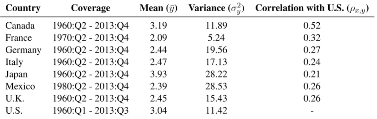
B.1 Sample Statistics . . . 61
B.2 Prior Distributions for the Two-state Model . . . 61
B.3 Prior Distributions for the Three-state Model . . . 61
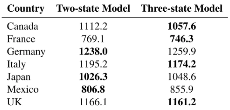
B.4 Bayesian Information Criterion . . . 62
B.5 Estimates for the Average Growth Rate and Variance Parameters . . . 62
B.6 Estimates for the Transition Probability Parameters. . . 63
B.7 Prior Specifications for Estimation . . . 63
B.8 Covariate Data Sources . . . 64
B.9 Growth Rates and Variance Parameters . . . 65
B.10 Hyperparameters for the Prior Distribution of Cluster Membership . . . 66
B.11 Cluster 3 Recession Dates and Major Events in Asia . . . 66
B.12 Transition Covariates Effects . . . 67
B.13 Priors for Estimation . . . 67
B.14 Transition Probabilities . . . 68
B.15 Cluster Composition . . . 69
LIST OF FIGURES
B.1 Real GDP Growth for Canada, Germany, and Japan . . . 71
B.2 Posterior Recession Probabilities . . . 72
B.3 Posterior Expansion Probabilities . . . 73
B.4 Posterior High-Growth Expansion Probabilities . . . 74
B.5 Marginal Effects on the Transition Probabilities for Canada . . . 75
B.6 Marginal Effects on the Transition Probabilities for France . . . 76
B.7 Marginal Effects on the Transition Probabilities for Germany . . . 77
B.8 Marginal Effects on the Transition Probabilities for Italy . . . 78
B.9 Marginal Effects on the Transition Probabilities for Japan . . . 79
B.10 Marginal Effects on the Transition Probabilities for Mexico . . . 80
B.11 Marginal Effects on the Transition Probabilities for the U.K. . . 81
B.12 Probability of Membership in Cluster 1 . . . 82
B.13 Probability of Membership in Cluster 1 Due to Cluster Covariates . . . 82
B.14 Probability of Membership in Cluster 2 . . . 83
B.15 Probability of Membership in Cluster 2 Due to Cluster Covariates . . . 83
B.16 Probability of Membership in Cluster 3 . . . 83
B.17 Probability of Membership in Cluster 3 Due to Cluster Covariates . . . 84
B.18 Posterior Recession Probabilities for Global Clusters . . . 85
B.19 Cluster 1 Recessions and the Euro Area Business Cycle. . . 86
B.20 Cluster 2 Recessions and the US Business Cycle . . . 86
CHAPTER 1
DOES THE UNITED STATES LEAD FOREIGN BUSINESS CYCLES?
1.1 Introduction
The U.S. is the largest of the world’s economies. In 2012, the U.S. accounted for 22.4 percent
of the world’s gross domestic product (GDP) and 35.1 percent of the world’s total market
capi-talization.1 The importance of the U.S. to the global economy was highlighted during the recent
Great Recession of 2007-2009. A financial shock originating for the most part in the U.S. led to a
worldwide downturn, which had detrimental and lasting effects on both developed and emerging
economies. This dynamic is summarized by the phrase, “when the U.S. sneezes, the rest of the
world catches a cold.”
Given this role as a global economic leader, a number of recent studies investigate the spillover
effects of the U.S. economy onto other nations. Arora and Vamvakidis (2004) use a fixed-effects
panel regression and find that U.S. economic growth has positive effects on the rest of the world,
especially for developing countries. Helbling et al. (2007) use multiple methodologies to
deter-mine the effect of the U.S. economy on other countries. By conducting an event study, they find
that U.S. recessionary periods coincide with global downturns. They also use simple regressions
while controlling for potential common unobserved shocks and country-specific effects and find
that a 1-percentage-point decline in U.S. growth leads to an average 0.16-percentage-point drop in
output growth across their sample of countries, with Canada, Latin America, and Caribbean
coun-tries being the most strongly influenced. Lastly, they use the more dynamic approach of structural
vector autoregressions (SVARs) to allow for both foreign and domestic effects, where they find
U.S. growth significantly impacts growth in Latin America, the Newly Industrialized Economies
(Hong Kong, Korea, Singapore, and Taiwan), and the Association of Southeast Asian Nations
(In-donesia, Malaysia, the Philippines, and Thailand). Antonakakis (2012) uses a dynamic measure of
correlation to examine the synchronization of G7 business cycles across a long time-series (1870
to 2011). They find U.S. recessions have positive effects on business cycle comovements after the
1971 breakdown of the Bretton-Woods system, with an increased level of synchronization during
the Great Recession.
The goal of this paper is to assess the influence that U.S. output growth has on the business
cycles of other nations. In particular, we ask if U.S. economic growth signals economic turning
points in other countries. In our setting, we cannot identify which structural innovations (shocks)
drive spillovers from the U.S. to other countries, or if the proximate shock leading to the turning
point is global in nature. Rather, we are merely interested in the comovement between U.S. output
and economic downturns of other countries. However, we do analyze the timing of when the U.S.
affects other countries. So, we could appeal to other studies as to what the driving forces were
during a given time period.2
Despite the inability of our model to offer a complete characterization of these shocks, our
study should be of relevant interest to policymakers and others interested in the dependence of
foreign business cycles on the U.S. economy. Our results imply that the trajectory of U.S.
out-put growth informs both the timing and duration of economic turning points in certain foreign
economies. Proper analysis of these cross-country linkages give policymakers, both in the U.S.
and abroad, a better understanding of the trade-offs faced when conducting independent and
coor-dinated actions.
Since our focus is on economic turning points, we use the regime-switching model of Hamilton
(1989) with time-varying transition probabilities (TVTP) as outlined by Goldfield and Quandt
(1973), Diebold et al. (1994), and Filardo (1994). This framework allows us to not only identify
economic turning points, but also the degree to which U.S. output growth influences the evolution
2For analysis of the specific mechanisms (trade openness, financial market linkages, etc.) by which the U.S.
of the underlying state—recession or expansion—of a nation’s economy. We consider
regime-switching models with both two (recession and expansion) and three states (recession, low-growth
expansion, and high-growth expansion).
Our panel of countries includes the Canada, France, Germany, Italy, Japan, Mexico, and the
United Kingdom (U.K.), covering the time period 1960:Q2 - 2013:Q4. We find that U.S. output
growth informs the timing and duration of recessions for Canada, Germany, the U.K., and, to a
lesser extent, Mexico. For the remaining countries (France, Italy, and Japan), we find no
relation-ship between U.S. output growth and business cycle turning points.
The paper proceeds as follows: Section 2.2 details the regime-switching model. Section 1.3
de-scribes the data and outlines the estimation methodology. Section 2.5 presents our results. Section
2.6 concludes.
1.2 Model
Burns and Mitchell (1946) characterized the business cycle as distinct phases of expansion and
recession. As defined by the National Bureau of Economic Research (NBER), a recession is a
wide-spread decline in economic activity typically lasting from a few months to over a year. On
the other hand, expansions are characterized by positive growth in economic activity and, typically,
longer durations.
Models of a country’s business cycle are typically estimated with that country’s data alone.
Regime shifts are characterized by sudden and persistent shifts in the growth rate of the economic
indicators, usually domestic GDP. In this paper, we are interested in contagion of economic
out-comes across countries. To this end, we will augment the standard business cycle model to account
for possible contagion by a dominant country—in this case, the U.S.
The model we adopt is based on the business cycle model of Hamilton, who characterizes the
cycle as a two-state process with random regime changes. In his framework, the mean growth rate
of a country’s output,yt, depends on a latent state variable, st={1,2}. The state of the economy
terms for simplicity, this model is given by
yt=
µ1+εt, ifst= 1(recession)
µ2+εt, ifst= 2(expansion)
,
where the error variance, εt ∼ N(0, σ2), is constant across states. Consistent with the NBER’s
definition of the business cycle, we restrict the average growth rate of output to be positive during
expansionary periods (µ2 >0) and negative during recessionary periods (µ1 <0).
In principle, we could include any number of states K in the model in order to better match
certain features of business cycles. For example, Kim and Piger (2000), Kim and Murray (2002),
and Billio et al. (2013) include three-states in their regime-switching model of the business cycle.
Additional states can reflect persistent differences in business cycle characteristics such as fast
versus slow growth expansion regimes or deep versus shallow recessions. The generalizedK-state
model is given by
yt =
µ1+εt ifst = 1,
µ2+εt ifst = 2,
.. . ...
µK +εt ifst =K,
with the identifying restrictionµ1 < µ2 < . . . < µK. We consider both a two-state (“recession”
and “expansion”) and a three-state (“recession”, “low-growth expansion”, and “high-growth
ex-pansion”) model for each country. We normalize the states such that µ1 < 0 < µ2 < µ3. This
provides econometric identification as well as an interpretations for future discussion.
1.2.1 Transition Probabilities
The NBER’s Business Cycle Dating Committee provides ex post historical dates for which
the U.S. is in expansion or recession. Many other countries do not have “official” business cycle
turning points. The model leaves the state of the economy unobserved, and, therefore, requires an
assumption about the evolution process of the state variable. Ideally, a model of economic business
and (2) expansions have longer average durations than recessions.
A standard assumption of regime-switching models is to assume the state variable follows a
first-order Markov process withfixedtransition probabilities (FTPs) [e.g., as in Hamilton (1989)].
The Markov property imposes that the current value of the state variable, st, is a function of its
previous value, st−1. In the two-state model, the transition matrix governing the Markov process
is represented as
P =
p11 p12
p21 p22
,
with FTPs
pji = Pr [st=j|st−1 =i], (1.1)
where the columns ofP each sum to 1(i.e., P
jpji = 1fori = 1,2). Thus, if a country was in
expansion last period (st−1 = 2), the probability that it remains in expansion this period (st = 2)
isp22, and the probability that the economy enters a recession this period (st = 1) isp12= 1−p22. Similarly, given that a country was in recession last period (st= 1), the probability that it remains
in recession this period (st = 1) is p11, and the probability the economy recovers and enters
expansion this period (st= 2) isp21 = 1−p11.
Persistence is generated in the Markov process when the diagonal elements of the transition
ma-trix are greater than the off-diagonal elements. Previous studies typically find the persistence
prob-ability of expansion,p22, to be greater than the persistence probability of recession,p11, coinciding
with the observation that the average duration of expansions is greater than that for recessions. For
example, Hamilton (1989) found a persistence probabilities for the U.S. of approximately 0.90 for
expansions and 0.75 for recessions, implying expected durations of 10 quarters for expansions and
4 quarters for recessions, similar to those defined by the NBER.
Because we are interested in how U.S. output growth informs economic turning points of other
nations, we extend Hamilton’s model to allow a foreign (U.S.) output growth rate to directly affect
the evolution of the underlying economic state of other nations.3 We assume the Markov process
is governed by time-varying transition probabilities (TVTP), which are functions of exogenous
covariates and last period’s state. In our case, we use the one-period lag of U.S. output growth,
yU S
t−1, as the single covariate which influences the switching process. The time-varying transition
matrix in the two-state model is
Pt=
p11,t p12,t
p21,t p22,t
,
with TVTP
pji,t= Pr
st=j|st−1 =i, yU St−1
= exp (αji+βjiy
U S t−1) 2
P
k=1
exp (αki+βkiytU S−1)
.
Here, αji is the time-invariant parameter and βji is the coefficient on lagged U.S. output growth.
The FTP model is nested under the TVTP framework if the covariate has no effect under each
state realization (i.e., βji = 0 fori = 1,2 andj = 1,2). Note that the time-invariant parameter
αji and the coefficientβji depend on both the previous state (st−1 = i) and the potential current
state (st = j) thereby reflecting the Markov property. Also, this parameterization allows U.S.
output growth to have asymmetric effects since we assume the coefficient is state dependent (i.e.,
βj1 6=βj2 forj = 1,2andβ1i 6= β2i fori = 1,2). In order to identify the transition parameters,
we must normalize one of the state’s transition parameters to be zeros. For the two-state model,
we use state 2: α2i = 0andβ2i = 0fori= 1,2.
For the generalK-state model, the time-varying transition matrix is
Pt=
p11,t p12,t . . . p1K,t
p21,t p22,t
..
. . ..
pK1,t pKK,t
, with TVTP
pji,t = Pr [st=j|st−1 =i,xt] =
exp (αji+βjiytU S−1) K
P
k=1
exp (αki+βkiyU St−1)
where we can impose the identification restrictions on state K: αKi = 0 and βKi = 0 for i =
1,2, . . . , K. We collect the unrestricted transition parameters into the[2K ×(K−1)]matrixΓ = [γ1, . . . , γK−1], whereγi = [αi1, . . . , αiK, βi1, . . . , βiK]
0
fori= 1, . . . , K −1. 1.2.2 Determining the Effects of U.S. Output Growth
The effect of U.S. output growth on other countries’ turning points appears to be summarized
by the coefficient βji in the transition equations. However, interpreting these coefficients in the
logistic framework of TVTP is less straightforward than in a simple linear regression model. One
of the ways to assess the effect of U.S. output growth on the transition dynamics is by looking at
the marginal effect of a change inytU S−1 on each transition probability pji,t for j = 1, . . . , K and
i = 1, . . . , K. We calculate the marginal effect of yU S
t−1 onpji,t by taking the partial derivative of
(1.2) with respect toyU S t−1:
∂pji,t
∂yU S t−1
=pji,t βji−β¯
,
whereβ¯=P
kpki,tβji is the probability weighted mean of the coefficient across states.
In the two-state model, the marginal effect of a change in yU S
t−1 on the probability of recession
(st = 1) simplifies to
∂p1i,t
∂yU S t−1
=β1ip1i,t(1−p1i,t),
which depends on the previous period’s state. Determining the sign of this marginal effect is
straightforward because it is irrespective of the value ofytU S−1 and therefore time-invariant. Ifβ1i <
β2i = 0, then the probability of experiencing a recession (expansion) next period falls (rises) as
lagged U.S. output growth rises. We expect to find this relationship for countries that tend to
comove with the U.S. economy. Conversely, ifβ1i > β2i = 0, then the probability of experiencing
a recession (expansion) next period rises (falls) as lagged U.S. output growth rises. We expect
to find this relationship for countries that move opposite (“decouple”) from the U.S. economy. If
β1i = β2i = 0, then the marginal effect is zero and lagged U.S. output growth does not influence
the transition probabilities. Therefore, no relationship exists between U.S. output growth and
economic turning points for the country under consideration.
because it depends on the value of yU St−1. For example, assume parameter values α11 = −1 and
β11 = −1 in a simple two-state version of our model (K = 2). First, consider the case where U.S. output growth is two-standard-deviations above its historical mean (yU S
t−1 = 2). Then, the
marginal effect of further changes in yU S
t−1 on the persistence probability of recession is -0.05.
However, if U.S. output growth is relatively low at two standard deviations below its historical
mean (yU S
t−1 =−2), then the absolute magnitude of this marginal effect quadruples to -0.20. Thus, the current status of the U.S. economy informs not only the probability of recession in the country
of interest, but also the current degree of influence U.S. output growth has over this probability.
In the general K-state model, both the sign and magnitude of the marginal effects depend on
the value of yU S
t−1. In order to fully assess the effect of U.S. output growth at different points in
time, we calculate the marginal effects over a range of possible values ofyU S t−1.
1.3 Data and Estimation
1.3.1 Data
We use the seasonally-adjusted, annualized quarter-to-quarter growth rate of real GDP as our
measure of economic activity growth (yt) for each country. We use the data from the Quarterly
Na-tional Accounts database provided by Organisation for Economic Co-operation and Development
(OECD). The countries included in our sample are the U.S.’ G7 counterparts (Canada, France,
Germany, Italy, Japan, and the U.K.) and Mexico, given its geographic proximity and economic
relationship with the U.S. Our time-series covers 1960:Q2 to 2013:Q4 for Canada, Germany, Italy,
Japan, and the U.K., 1970:Q2 to 2013:Q4 for France, and 1980:Q2 to 2013:Q4 for Mexico. Table
B.1 provides summary statistics for our sample.
For the transition covariate, ytU S−1, we use the one period lag of U.S. output growth from the
OECD’s Quarterly National Accounts database, covering the time period 1960:Q1 to 2013:Q3. To
simplify the interpretation of the results, we standardize the time series of U.S. output growth to
have zero mean and unit variance. Thus, yU S
t−1 = 0 implies the U.S. is at its historical average
growth rate over our sample period, approximately 3.04%. Similarly, yU S
t−1 = cmeans the U.S.
is growing at c standard deviations away from its historical average growth rate. For example,
yU S
output growth from 1960:Q1 to 2013:Q2 is approximately 3.38.
Figure B.1 plots the time-series of real GDP growth for a subset of our sample (Canada,
Ger-many, and Japan). Grey bars represent U.S. recession dates as defined by the NBER’s Business
Cycle Dating Committee and are included only for reference. For each country, real GDP growth
tends to fall during periods of U.S. recession, implying some connection between U.S. and other
countries’ growth.
1.3.2 Estimation
We estimate both the two- and three-state models using the Gibbs sampler, a Markov-chain
Monte Carlo algorithm used in a Bayesian environment. Rather than drawing from the full joint
posterior distribution directly, the Gibbs sampler draws each of the four parameter blocks from
their individual conditional posterior distribution given the draws for the other blocks. First, we
partition the parameters and latent variables into four blocks: (1) the average growth rates µ =
[µ1, . . . , µK]
0
; (2) the error variance σ2; (3) the transition probability parameters Γ; and (4) the
time-series of the latent state variable,s= [s1, . . . , sT]
0
. We run the sampler for 100,000 iterations,
discarding the first 50,000 to achieve convergence.
Prior distributions for the parameters of the two- and three-state model are given in Tables
B.2 and B.3, respectively. In each case, we use conjugate prior distributions. Following Kim
and Nelson (1999), the steps to draw the average growth rate and error variance parameters are
straightforward. The conditional posterior distribution for the vector of average growth rates,µ, is
multivariate normal and the posterior for the error variance,σ2, is inverse-Gamma.
The transition probability parameters can be rewritten as a differences in random utility model
(dRUM) as outlined by Fr¨uhwirth-Schnatter and Fr¨uhwirth (2010) and Kaufmann (2011). Under
the dRUM, we assume each state has a continuous, latent utility value. Conditional on knowing
the state at each point in time, the observed state is the one with the highest utility. The conditional
posterior distribution of the transition parameter vector, γi,is multivariate normal for each state
i = 1, . . . , K −1. The unobserved state variable is drawn using the filter from Hamilton (1989) with the smoothing algorithm from Kim (1994). For the generalK-state model, we use the
Choosing between using two states (“recession” and “expansion”) and three states (“recession”,
“low-growth expansion”, and “high-growth expansion”) is a model selection problem. We use
Bayesian Information Criterion (BIC) to choose which model is best suited for each country. BIC
is calculated as
BIC =−2 log[L(Θ,s,y,yU S)] +Nlog(T)
whereN is the number of parameters in the model,T is the number of time-series observations, and
L(Θ,s,y,yU S)is the value of the likelihood function given model parametersΘ = {µ, σ2, α, β}, the state vector s, and the data y = [y1, . . . , yT] and yU S =
y0U S, . . . , yTU S−1. BIC accounts
for the likelihood of the data, while penalizing models with a large number of parameters. BIC
was shown by Raftery (1995) and Kass and Raftery (1995) to approximate the Bayes factor of
competing models, and thus provides an adequate solution to our model selection issue. The BIC
is calculated at each iteration of the Gibbs sampler and the optimal model for each country is the
one which minimizes the median BIC calculation.
1.4 Results
Table B.4 gives the model selection results for each country. The two-state model is preferred
for Germany, Japan, and Mexico, while the three-state model is chosen for Canada, France, Italy,
and the U.K. These results suggest a more stable expansion output growth rate for the former
countries, while the latter countries appear to have both low and high growth expansions.
We present the estimated mean growth rate and variance parameters for each country in Table
B.5. Germany, Japan, and Mexico each have much higher error variance than the other countries
in sample, possibly due to the lack of third state in their optimal model to capture high-growth
dynamics. The lack of two expansion states also explains the higher estimated mean expansionary
growth rate for these countries since it is capturing episodes of both high- and low-growth.
We discuss the remaining results in two subsections. The first outlines the estimated recession
timing for each country across time. The second subsection assesses the ability of U.S. output
1.4.1 Timing of Business Cycle Phases
Figure B.2 presents the probability implied by our model that a country is in a state of
reces-sion at each time period in our sample. In technical terms, these are the posterior probability of
recession,Pr[st = 1|ΩT]for each country conditional on ΩT, the information at timet. For each
t, Pr[st = 1|ΩT]is the percentage of Gibbs iterations for which a recession state is drawn at each
time period. Although all of the countries in our sample experience some similar recessions (e.g.,
the first oil crisis of the mid 1970’s and the Great Recession of 2007-2009), there are substantive
differences in the timing of entering recessions as well as their durations. For example, we find
that most countries enter recession after the NBER determined that the Great Recession of
2007-2009 in U.S. already began. Although some countries (e.g., Canada, Mexico, and the U.K.) exit
this recession with the U.S., others (e.g., Italy and Japan) experience lasting effects of the global
downturn leading to a “double-dip” recession.
For completeness, we plot the posterior probability of expansion in Figure B.3. Countries
following the two-state model (Germany, Japan, and Mexico) have a single expansion state and
therefore a single posterior probability of expansion, whereas countries following the three-state
model (Canada, France, Italy, and the U.K.) have two expansion states (low- and high-growth).
For the latter, we include the posterior probabilities of the low-growth expansion state in Figure
B.3 and we plot separately the posterior probabilities for the high-growth state in Figure B.4.
Consistent with the empirical literature on business cycles, we find the expansion state(s) to
be highly persistent with longer average duration(s) than the recession state. The high-growth
expansion state accounts for periods of relatively high-growth prior to 1985, the beginning of the
period known as the Great Moderation. For France, the high-growth expansion state also captures
two notable economic periods: the movement away from dirigisme in the late 1980s, and the
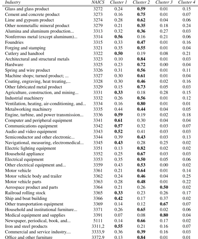
1.4.2 Does U.S. output growth drive business cycles?
The focus of this paper is on whether U.S. output growth informs economic turning points of
other nations.4 In our modelling framework, this relationship is captured in the transition dynamics
of the state variable. Table B.6 displays the median posterior draws for the transition probability
parameters for all the countries in our sample. As we noted in Section 1.2.2, the coefficientsβji
in the transition equations suggest how U.S. output growth influences the state dynamics of the
country of interest. They are not, however, the sole determinants of the (marginal) effect of a
change in lagged U.S. output growth on the transition probabilities on the business cycle of a given
country. Because the marginal effects depend on both the value of lagged U.S. output growthytU S−1
and the previous state of the economy st−1, we calculate them across all possible combinations
of st−1 and ytU S−1.5 We do this for each iteration of the Gibbs sampler, thereby constructing the
posterior distribution for each of the marginal effects.
Figures B.5 through B.11 display the marginal effect of a change in lagged U.S. output growth
on each of the transition probabilities. The horizontal axis for each figure reflects different values
for U.S. output growth, negative four to positive four standard deviations from its historical
aver-age. The vertical axis plots the marginal effect of a change in U.S. output growth on the respective
transition probability conditional on the value forytU S−1 and the previous statest−1. In each figure,
the blue line represents the posterior median of the marginal effect and the shaded region represents
the 68% coverage of the posterior distribution.
A positive marginal effect implies that an increase in lagged U.S. output growth increases the
respective transition probabilitypji,t = Pr(st=j|st−1 =i, ytU S−1). Conversely, a negative marginal effect implies that an increase in lagged U.S. output growth decreases the respective transition
probability. That is, for countries that comove with the U.S., we expect to find a positive (negative)
4Note that we cannot infer causality of the business cycle in the structural sense, but rather we assess if U.S. output
acts as an informative indicator of other countries’ turning points. Therefore, countries for which our model indicates that U.S. output growth is not a significant indicator does not imply a lack of structural mechanisms which propagate shocks between the two nations.
5We consider values foryU S
t−1between negative four standard deviations and positive four standard deviations of
marginal effect of yU St−1 on the probability of transitioning to an expansion (recession) and the
persistence of expansion (recession). For countries that decouple from the U.S., we expect to find
a negative (positive) marginal effect of yU S
t−1 on the probability of transitioning to an expansion
(recession) and the persistence of expansion (recession).
For each country, we assess the ability of U.S. output growth to inform (1) the timing of
en-tering a recession, (2) the persistence or duration of a recession, and (3) transitions between states
of low- and high- growth expansion (for countries following the three-state model). We assess the
first dynamic by looking at the marginal effect of U.S. output growth on the transition probability
from expansion (st−1 = 2 or 3) to recession (st−1 = 1), so the relevant transition probabilities
arep12,t andp13,t. For recession persistence, we see if U.S. output influences the transition
prob-ability of staying in recession this period (st = 1) given the economy was in recession last period
(st−1 = 1) with relevant transition probability p11,t.We analyze the the last aspect by looking at
both the persistence probability of both low- (p22,t) and high-expansion (p33,t) states in addition to
the transition probabilities between the two expansion states (p23,t andp32,t).
The three countries for which U.S. output growth has the most influence are Canada, Germany,
and the U.K.. For these countries, lagged U.S. output growth influences both the timing of entering
a recession as well as the duration of a recession. The results show that each of these countries
comove with the U.S.: higher U.S. output growth implies a lower probability of recession, and
lower output growth implies a higher probability of recession (↑ yU S
t−1 ⇒↓ p1i,t, ↑ p2i,t for all i).
Figure B.7 presents the marginal effects for Germany, which follows the simpler two-state model.
For Germany, the marginal effect of U.S. output growth is largest (in absolute terms) at low levels
of ytU S−1, or when the U.S. is likely in a state of recession. Therefore when the U.S. economy is
in dire circumstances (as signalled by low output growth), Germany is more susceptible to any
further movements in U.S. output relative to more “normal” economic times.
In addition to informing the timing and duration of recessions, U.S. output growth also
influ-ences the transition dynamics of low- and high-growth expansion for Canada, as seen in Figure
B.5. When U.S. growth is relatively low (i.e., below its historical mean), increases in U.S. output
is relatively high (i.e., above its historical mean), increases in U.S. output growth decrease the
persistence of low-growth expansion and increase the probability of transitioning to high-growth
expansion (↑p32,t) -as well as the persistence probability of high-growth expansion (↑p33,t). This
result reflects the strong economic relationship between Canada and the U.S. since it not only
informs the timing of recessions but also the timing of varying degrees of expansion.
For Mexico, lagged U.S. output growth informs the duration of recession but not the timing
of entering recession. When U.S. output growth falls, the persistence probability of recession in
Mexico rises (↑ p11,t) implying a longer expected duration of recession. The lack of U.S. output
growth influencing the timing of Mexico entering recession could be due to the fact that Mexico
experienced idiosyncratic recessions unrelated to the U.S. (e.g. the 1994 Mexican peso crisis),
which tended to be shorter than coincident recessions with the U.S. (e.g. the recession of the early
1980’s and the Great Recession of 2007-2009).
The results for France, Italy, and Japan suggest that lagged U.S. output growth does not
influ-ence the timing or duration of recession for these countries. For France and Italy, increases in U.S.
output growth increase the persistence probability of high-growth expansion (↑ p33,t), but only at
low-levels of U.S. output growth.
Recent studies on business cycle synchronization offer two possible explanations of our results:
stage of development and common language. Regarding the first explanation, Kose et al. (2012)
find that emerging market economies and advanced economies have decoupled during the
global-ization period but countries inside each respective group have converged. This finding is consistent
with our result that the U.S. is more informative for the business cycles of advanced countries like
Canada, Germany, and the U.K., and less so for the developing country in our sample, Mexico.
Another plausible explanation is that countries with a common language tend to have similar
business cycles.6 We find that U.S. output growth informs the business cycles for each of the
countries in our sample with English as thede factoor official language.
1.5 Conclusion
In this paper, we assessed whether U.S. economy drives business cycle turning points of other
nations. We extended the nonlinear business cycle model of Hamilton (1989) to allow U.S. output
growth to influence the probability of a country moving between states of expansion and recession.
We found that the U.S. does inform the timing and duration of recessions for Canada, Germany, the
U.K., and, to a lesser extent, Mexico. Additionally, we found no informative relationship between
U.S. output growth and the business cycles of France, Italy, and Japan.
It is important to keep in mind that the results here suggest only that the U.S. does not appear to
lead France, Italy, and Japan. If these countries business cycles react intraquarter to fluctuations in
U.S. output, they would show up as a false negative in the estimation. Further, if a common world
shock affects the U.S. before other countries, the result might be a false positive. However, our
analysis provides a framework for approaching the question of Granger causality across business
CHAPTER 2
BUSINESS CYCLES ACROSS SPACE AND TIME
2.1 Introduction
Recent evidence suggests the presence of an overarching world business cycle with a number of
underlying regional business cycles.1 For instance, all countries experience global shocks, such as
the financial crisis of 2009, but only a subset of countries experience idiosyncratic regional shocks,
such as the European debt crisis which began in 2011. This paper seeks to answer a number of
questions regarding how the world business cycle interacts with less-pervasive business cycles that
are isolated to a subset of countries: How has this relationship between global and regional cycles
evolved over time? What factors determine business cycle similarities across countries? What
drives international turning points?
One way to model the business cycle is as a movement between distinct latent states of
expan-sion and recesexpan-sion [see Burns and Mitchell (1946)].2 Distinguishing periods of recession can be
done through a simple rule such as two consecutive periods of economic contraction, or through
richer statistical methods. For example, Hamilton (1989) outlined a two-state Markov-switching
model of the U.S. economy and found similar recession dates to those outlined by the NBER. Since
that seminal paper, numerous studies have implemented Markov-switching frameworks to estimate
1Kose, Otrok, and Whiteman (2003, 2008) determined that both regional and global factors account for a relatively
large portion of the variation in economic growth across countries. Bordo and Helbling (2011) conducted historical analysis of international business cycle synchronization over the past , and similarly found an increase in the impor-tance of global shocks over time. On the other hand, Kose, Otrok, and Prasad (2012) and Hirata, Kose, and Otrok (2012) found a decline in the importance of global factors, but an increase in business cycle comovement within both emerging and developing economies.
2Alternatively, there is a large literature on modelling business cycles through dynamic factors as opposed to
business cycle phases for multiple economies and compare common movementsex post.3
Typi-cally these studies assume independence across economies where individual cycles are estimated
separately from one another in a univariate setting. These univariate Markov-switching models
therefore do not lend themselves to properly analyze the comovement and interaction of multiple
economies.
Hamilton and Owyang (2012, henceforth HO) constructed a regional business cycle model to
consider a large number of economies inside of a single Markov-switching framework. In their
ap-plication, they analyze the U.S. national business cycle and its interaction with state-level business
cycles. To alleviate the parameter proliferation problem associated with using a large cross-section,
HO implement time-series clustering by assuming that states tend to move together in a small
num-ber of endogenously-determined groupings determined by historical employment growth rates and
other state-specific characteristics, such as industry composition. They find evidence that all states
tend to experience national downturns, but the specific timing of entering or exiting recession
dif-fers depending on the shock which initially led to the downturn.
A shortfall of HO’s model is that they assume the underlying business cycle regime evolves
according to fixed transition probabilities (FTP). Markov-switching models with FTP (e.g.,
Hamil-ton, 1989; HO) assume the current regime is a function of only the previous regime(s), and may
miss vital information (contained in macroeconomic data) signalling business cycle turning points.
For example, the probability of a global recession should rise when there is a financial crisis. To
reflect this, the variables driving the time-variation of the transition probabilities should contain
financial statistics informing the model of an impending downturn.
We adopt the framework of HO and apply it to countries rather than states, with the primary
methodological innovation being the inclusion of time-varying transition probabilities (TVTP).
Markov-switching models with TVTP have two particular advantages over standard fixed
transi-tion alternatives. First, the economic regime is a functransi-tion of both the previous regime as well as
past macroeconomic conditions. We can therefore include a set of covariates which inform the
3See Owyang, Piger, and Wall (2005), Owyang, Piger, Wall, and Wheeler (2008) and Altu˘g and Bildirici (2012),
model of the timing of regime switches. The second advantage of using TVTP is that the expected
duration of a given state is also time-varying. This feature is more intuitive than models with
con-stant expected duration (i.e., models with FTP) because recessions tend to have different lengths
depending on the economic climate and their proximate causes. For example, economists expect
that a recession caused by a negative financial shock will last longer than a recession due to say a
contractionary oil shock. Similarly, the expected length of a recession should depend on the
rela-tive magnitudes of the underlying shocks. For example, a large shock to oil prices implies a longer
expected recession relative to a much smaller oil price shock.
Since it is infeasible to include every variable believed to influence international turning points,
the choice of which variables to include in the switching process is crucial to the model’s
impli-cations. For this study, we choose four variables which economic theory and previous empirical
studies determined to have predictive ability and substantive relationships with previous
reces-sions. These include term spreads, oil price shocks, global stock market returns, and global house
price movements.
We use the Bayesian technique of Gibbs sampling to perform posterior inference. Our dataset
includes 37 countries, covering the time period of 1970:Q3 - 2013:Q2. In that time frame, we
find two instances of global recession: the first oil crisis in 1974 - 1975 and the global financial
crisis of 2008 - 2009. We find three groups of countries, or “clusters,” which tend to experience
their own independent timing of recessions. As previous studies suggest, geographic proximity is
an important factor in determining the groupings of these countries.4 However, we find that trade
openness, industrialization, and similar institutional factors, such as linguistic diversity are also
important.
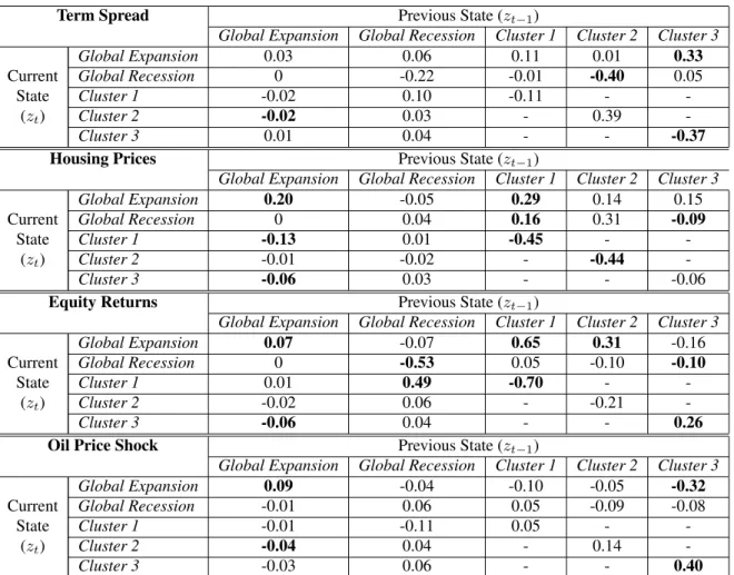
From the TVTP setup, our results suggest that the primary drivers of international turning
points are movements in asset prices. We do not find that any one cluster is particularly exposed
to a single type of shock, but rather idiosyncratic recession timing across all clusters depends upon
4We should note this result comes from analyzing the cluster compositions ex postand finding a tendency of
fluctuations in asset prices. This result reinforces the finding by Reinhart and Rogoff (2009) and
Helbling et al (2011) of the importance of financial markets in propagating recessions to a global
level.
The outline of the paper is as follows: Section 2.2 outlines the model. Section 2.3 explains the
estimation technique. Section 2.4 describes the data. Section 2.5 presents the estimation results
and findings. Section 2.6 concludes the paper.
2.2 Model
The central framework of our model is the multivariate regime-switching framework of
Hamil-ton and Owyang (2012, HO). We assume each economy’s growth rate depends on a latent regime
indicator which takes one of two possible states at each time period. These states represent the
business cycle, with alternating phases of expansion and recession. In expansion states, the
econ-omy grows at a relatively higher average rate than in recession states.
Standard regime-switching models (e.g., Hamilton, 1989; HO) assume the regime indicator
follows a first-order Markov process with fixed transition probabilities (FTP). Here, the
proba-bility of the current period’s state (i.e., expansion or recession) depends upon last period’s state,
allowing the model to capture regime persistence. For example, Hamilton (1989) found in a
sim-ple one-country model that expansionary periods tend to be followed by expansionary periods and
recessionary periods tend to be followed by recessionary periods. This characteristic matches the
dating of recessions by the NBER’s Business Cycle Dating Committee.
However, the regime-switching model with FTP has a number of shortcomings. First, the
evo-lution of the regime is an implicit probabilistic process. The model is parsimonious and tractable,
but operates as a “black box” with underlying dynamics that may be of interest to researchers and
policymakers. Second, regime persistence is constant across time periods. A framework wherein
the expected duration of a regime (e.g., a recession) is a function of current economic conditions
is more appealing. Therefore, we assume the switching process for the aggregate regime variable
follows time-varying transition probabilities (TVTP).5 In the model with TVTP, the underlying
5Time-varying transition probabilities were first considered by Diebold, Lee, and Weinbach (1994), Filardo (1994),
transition probabilities are a function of exogenous transition covariates, in addition to the
previ-ous state. In our application, the transition covariates are measures of global shocks and economic
conditions informing the timing of business cycle turning points. The inclusion of TVTP in the
regime-switching process allows us to consider what shocks tend to drive groups of countries into
and out of recession.
In addition to the modeling assumptions placed on the transition dynamics, we must also
consider the interaction of business cycles across countries. Typically, regime-switching
mod-els which consider multiple countries assume either full dependence or full independence across
country business cycles. In the case of full dependence, all countries follow the same cycle and
can therefore be summarized by a single, global regime indicator. Conversely in the case of full
independence, each country’s cycle is estimated separately from the others’ and assumes that each
country’s business cycle state offers no information for other countries’ states. We opt for an
in-termediate assumption wherein we model a global business cycle while allowing for deviations for
groups of countries, or what we call “clusters”. Following HO and Francis, Owyang, and Savas¸c¸in
(2012, henceforth FOS), we determine cluster composition endogenously through similar
move-ments in economic growth as well as a set of country-specific characteristics which enter through
the prior distribution.
LetN be the number of countries considered in the model. Let ynt be the growth rate of real
GDP for countrynat time periodt. Letsntbe countryn’s business cycle regime indicator:snt = 1
if in recession, andsnt = 0if in expansion. Countryn’s average growth rate in expansion isµ0n,
and the average growth rate in recession isµ0n+µ1n. The multi-country regime-switching model
is given by
yt=µ0+µ1st+εt, εt i.i.d
∼ N(0,Σ), (2.1)
whereyt = [y1t, . . . , yN t]0, st = [s1t, . . . , sN t]0, µ0 = [µ01, . . . , µ0N]
0
, µ1 = [µ11, . . . , µ1N]
0 , and
εt = [ε1t, . . . , εN t]
0
. The symbolrepresents element-by-element multiplication.
We assume the error vector εt is independent of the state vector,sτ, for all time periods (i.e.
E[ε0tsτ] = 0∀τ). Additionally, we assume the covariance matrix is diagonal :Σ=diag(σ12, . . . , σN2 ).
This assumption implies that coincident recessions are the only channel through which economic
growth is correlated across countries. Therefore, business cycle synchronization shows up as
sim-ilar recession timing reflected in the regime vectorstin our model.
2.2.1 Clustering
Each country’s regime indicator can take one of two possible values at any given time period
(0 for expansion or 1 for recession). When the number of countries (N) is large, the regime vector
stcan take2N possible values. Left unrestricted, the model cannot be feasibly estimated due to the
number of possible combinations the regime vector can take and the resulting parameter
prolifera-tion problem. One potential soluprolifera-tion is to assume all of the country cycles are fully dependent, and
therefore follow the same global business cycle. Conversely, we could assume full independence
across country cycles and estimate each individual country’s regime variable independent of the
others’.6
Instead we opt for an assumption between the case of full dependence and full independence.
We restrict the number of possible values for the regime vector through a time-series clustering
framework.7 Clustering assumes there are a number of unobserved groupings – or, “clusters” –
of countries which experience similar business cycle turning points apart from the global cycle.
Country-members of each respective group experience idiosyncratic recessionary periods while
non-members are in expansion. It is important to note that this assumption abstracts away from
business cycle turning points isolated to a single country or a small group of countries. Therefore,
recessions must be substantially pervasive across countries in order to show up in our model. This
assumption is justified by the recent empirical evidence from Kose et al. (2012), which suggests
that a large portion of economic growth is due to both global and regional factors.
6Full independence implies that for two countries A andB, the business cycle regimes for each country s A,t
andsB,tsatisfy Pr (sA,t=i, sB,t=j) = Pr (sA,t=i) Pr (sB,t=j). Or equivalently, Pr (sA,t=i|sB,t=j) = Pr (sA,t=i).
7See Fr¨uhwirth-Schnatter and Kaufmann (2008), HO, FOS, and Hern´andez-Murillo et al. (2013). The time-series
clustering framework reduces these possible values toK+ 2(whereK+ 2<<2N), giving us a numerically tractable
Assume there is an aggregate latent regime variablezt∈ {1, . . . , K, K + 1, K+ 2}indicating
which cluster of countries is in recession at timet. Associated with each aggregate statezt = k
is a(N ×1)vectorhk = [h1k, . . . , hN k]0, wherehnk = 1when countrynis a member of cluster
k and hnk = 0 when country n is not a member of clusterk. Thus, we refer tohnk as a cluster
membership indicator.
Selecting theK+ 2clusters to include out of the2N possible combinations is a model selection
issue. We opt to always include the two “global” clusters; when all countries are simultaneously
in either recession or expansion. Ex ante, we associate these global clusters with the aggregate
regimeszt =K+ 1(all countries in recession,hK+1 = [1, . . . ,1]0) andzt =K + 2(all countries
in expansion,hK+2 = [0, . . . ,0]0).
For the remaining aggregate regimeszt = 1, . . . , K, a group of countries is in recession while
simultaneously all remaining countries are in expansion. These regimes are associated with what
we call “idiosyncratic” clusters since one group of countries experiences an idiosyncratic
reces-sion in relation to the rest of the countries in our sample when these regimes are realized. Country
membership hnk in each of the idiosyncratic clusters is an unobserved variable determined
en-dogenously. We infer cluster membership from similar movements in economic growth as well
as country-specific covariates which enter through a hierarchal prior specification. Following
FOS, we restrict each country to be a member of one and only one idiosyncratic cluster (i.e.,
PK
k=1hnk = 1). This assumption stands in contrast to the model of HO, which did not restrict U.S.
states to a single cluster, but allowed for each state to be a member of either one cluster, multiple
clusters, or none of the clusters. Our assumption uncovers the “strongest” comovement
relation-ships across countries, whereas leaving cluster membership unrestricted offers the flexibility to
capture relatively weaker instances of economic comovement.
We rewrite (2.1) as a mixture model withK+ 2components:
where
mk =µ0+µ1hk.
2.2.2 Evolution of the Regime
We assume the switching process for the aggregate regime variable zt follows time-varying
transition probabilities(TVTP). The underlying transition probabilities are a function of a set of
transition covariates vt = [v1t, . . . , vLt]
0
in addition to the realization of last period’s state zt−1.
Following Kaufmann (2011), we adopt a centered parameterization in order to properly identify
the time-varying and time-invariant portions of the transition probabilities. Formally, the TVTP
takes the multinomial logistic representation:
pji,t= Pr(zt=j|zt =i,vt) =
exp
(vt−¯v)γjiv +γji
PK+2
k=1 exp [(vt−v¯)γ v
ki+γki]
, (2.3)
whereγjiv is a(L×1)vector of coefficients for the transition covariates andγjiis the time-invariant
transition parameter.8 We set the arbitrary threshold vector¯vto be the mean of the covariates. For
identification purposes, we define stateK + 2as the reference state, implyingγKv+2,i =0L+1 and
γK+2,i= 0for alli= 1, . . . , K + 2. We compile the transition probabilities at time periodtin the
transition matrixPt, wherepji,t is the element in thejth row andith column.
We impose the identifying restrictionsµ0n≥0andµ1n<0for alln. These restrictions identify
the business cycles states by ensuring that on average countries grow faster during expansions
relative to recessions.9 We also need the restrictions to avoid label switching between the two
worldwide states and two growth rate parameters during estimation.
In order to identify the idiosyncratic clusters, we must impose restrictions on the transitions of
the aggregate state variable, zt. Following HO, we deny transitions from one idiosyncratic state
to a different idiosyncratic state by imposingpji,t = 0for all twherei 6= j, i ≤ K, andj ≤ K.
8Note that the framework with time-varying transition probabilities nests the simplier fixed transition probability
setup. In the FTP case,γv
ji=0for alli,j.
9Notice that we do not restrict the average growth rate in recessionary periods (µ
0n+µ1n), thus allowing for the
Thus, individual clusters experience idiosyncratic recessions relative to the world, but not directly
following another cluster experiencing its own idiosyncratic recession in the previous period. This
assumption focuses our attention on cluster deviations from the global business cycle (rather than
between clusters) and significantly reduces the number of parameters to be estimated.
2.3 Estimation
We use the Bayesian technique of Gibbs sampling [Gefland and Smith (1990), Casella and
George (1992), Carter and Kohn (1994)] to estimate the model. Gibbs sampling is a Markov-chain
Monte Carlo (MCMC) technique which separates the model parameters and latent variables into
blocks. Each block is drawn from their conditional posterior distributions rather than directly
draw-ing from the unconditional joint posterior density. This method is particularly useful in instances
where it is difficult or infeasible to sample directly from the full joint posterior distribution, as is
the case with our model.
We have a total of four blocks to be estimated. The first block is the entire set of growth
and variance parameters,θ ={θ1, . . . , θN}, where θn = {µn0, µn1, σn2}. The second block is the
aggregate state time series,Z={z1, . . . , zT}. The third block consists of the entire set of transition
probability parameters,γ = {γ1, . . . , γK+2}, where γj =
γjv10, γj1, . . . , γjKv0 +2, γjK+2 0
represents
the entire set of transition parameters governing the transition probabilities to state j. The fourth
block,H={β, ξ, λ, h},includes the cluster membership indicators,h={h1, . . . ,hK+2}, as well as the set of hyperparameters and latent variables determining the prior for cluster association,
β ={β1, . . . , βK+2},ξ ={ξ1, . . . , ξK+2}, andλ={λ1, . . . , λK+2}.10 2.3.1 Priors
We must define prior distributions for the parameters. These distributions are given in Table
B.7. The mean growth rate parameters have a normal prior distribution. The variance parameters
have an inverse-Gamma prior distribution. Following Kaufmann (2011), the transition parameters
have a normal prior distribution.
Following Fr¨uhwirth-Schnatter and Kaufmann (2008), HO, Francis, Owyang, and Savas¸c¸in
10Note:ξ
(2012), and Hern´andez-Murillo et al. (2013), we assume that country n’s prior probability of
membership in idiosyncratic clusterk = 1, . . . , K depends on a(Q×1)country-specific cluster covariate vector,xnk:
p(hnk) =
exp(x0nkβk)
1+exp(x0nkβk) ifhnk = 1
1
1+exp(x0nkβk) ifhnk = 0
. (2.4)
This assumption allows countries to endogenously cluster based on comovements in real GDP
growth and country-specific covariates rather than imposing country groupings exogenously.
Fol-lowing Holmes and Held (2006) and HO, we rewrite (2.4) under the assumption that cluster
mem-bership is determined by an underlying latent variableξnk with associated varianceλnk:
hnk =
1 ifξnk >0
0 else
,
where
ξnk|βk, λnk ∼N(x0nkβk, λnk)
λnk = 4ψnk2
ψnk ∼KS,
whereKS represents the distribution of the Kolmogorov-Smirnov test statistic.
2.3.2 Posterior Inference
In this section, we give a brief overview of the posterior draws. Appendix A outlines the
specifics of each sampling step in further detail.
We draw each country’s individual parameter set θn = {µn0, µn1, σn2} conditional on
know-ing all other countries’ parameter values. The posterior distribution for a country’s mean growth
rates is multivariate normal, while the posterior for a country’s variance is inverse-Gamma. This
sampling step is standard for Markov-switching models [see Kim and Nelson (1999)].
The latent state vector,Z, is drawn conditional on the other model parameters. We implement
combine the mutiple-state extension of the filter – outlined by HO – with the inclusion of TVTP as
in Kaufmann (2011).
We utilize the difference random utility model (dRUM) outlined by Fr¨uhwirth-Schnatter and
Fr¨uhwirth (2010) and Kaufmann (2011) to sample the transition probability parameters ,γ. The
dRUM is a data augmentation method that gives us a linear regression of γj with logistic errors.
The logistic errors can be approximated by a mixture of normal distributions, so that the
pos-terior distribution for γj is normal conditional on knowing the state vector and the other states’
transition parameters. After drawing the entire set of transition parameters, we calculate the
tran-sition probabilities at each point in time and obtain the entire time series of trantran-sition matrices,
P={P1, . . . , PT}.
Cluster membership and the associated prior hyperparameters are drawn in four substeps. We
first draw the coefficients in the prior,βk, from a normal distribution conditional on knowing the
other model parameters and prior hyperparameters. Following Holmes and Held (2006), we draw
the latent variableξnk from a truncated logistic distribution. We then draw the variance of this
dis-tribution,λnk, conditional on this new draw ofξnk. Countryn’s idiosyncratic cluster membership
indicator,hnk, is drawn conditioned on the membership indicators for the other countries and the
new parameter draws. After incorporating the hierarchical prior, cluster membership depends on
similarity in fluctuations across countries’ economic growth rates.
2.3.3 Choosing the Number of Clusters
Determining the optimal number of idiosyncratic clusters, K, is a model selection problem.
Ideally, we would calculate the marginal likelihoodp(Y|Θ)across a number of potential idiosyn-cratic clusters. HO implement cross-validation to approximate the marginal likelihood of different
models. Cross-validation is computationally intensive since it involves testing the out-of-sample fit
of each model to approximate its marginal likelihood. Hern´andez-Murillo et al. (2013) determine
the optimal number of clusters based on Bayesian Information Criterion (BIC), which was shown
by Kass and Raftery (1995) to well-approximate the marginal likelihood.
latent variables. McLachlan and Peel (2010) find through simulations that BIC may overrate
mod-els with a large number of clusters. Thus, we also calculate the Integrated Classification Criterion
(ICL-BIC) which penalizes models for both complexity and the presence of overlapping clusters.
Since these information criterion are decreasing with the likelihood and increasing in the penalty
factors (complexity and/or overlapping clusters), the optimal number of clusters is the model with
the smallest BIC or ICL-BIC.
2.4 Data
We use quarterly real GDP growth as our indicator of economic activity for each country. Our
sample includes 37 countries11 covering the time period 1970:Q3 - 2013:Q2. For a majority of the
advanced economies, we use the OECD’s Quarterly National Accounts dataset. We supplement
this with Oxford Economics’ (henceforth OE) Global Economic Databank, which provides real
GDP data for many of the developing and emerging economies of our sample.12 The OE data
runs from 1980:Q1 - 2013:Q2 which results in an unbalanced panel when grouped with the OECD
dataset.13
In order to control for the Great Recession, we allow for a structural break in the average
growth rates beginning in the first quarter of 2008 through the third quarter of 2009. We represent
this break by rewriting (2.2) as:
yt|zt=k∼N(m∗k,Σ)fork= 1, . . . , K+ 2,
11Countries included in our sample include Argentina, Australia, Austria, Belgium, Brazil, Canada, Chile, China,
Denmark, Finland, France, Germany, Hong Kong, India, Indonesia, Ireland, Italy, Japan, Korea, Luxembourg, Malaysia, Mexico, Netherland, New Zealand, Norway, Philippines, Portugal, Singapore, South Africa, Spain Swe-den, Switzerland, Taiwan, Thailand, United Kingdom, United States, and Venezuela.
12The OECD provides data for Australia, Austria, Belgium, Canada, Denmark, Finland, France, Germany, Ireland,
Italy, Japan, Luxembourg, Netherlands, New Zealand, Norway, Portugal, South Korea, Spain, Sweden, Switzerland, United Kingdom, and the United States. The OE dataset includes Argentina, Brazil, Chile, China, Hong Kong, India, Indonesia, Malaysia, Mexico, Philippines, Singapore, South Africa, Thailand, and Venezuela.
13Previous studies on international business cycles use data from the Penn World Tables which would allow us to
where
m∗k = (µ0+Dtµ∗0) + (µ1+Dtµ∗1)hk.
andDtis a dummy variable which is equal to 1 during the Great Recession time period (2008:Q1
-2009:Q3) and 0 otherwise. This specification controls for the potential structural break during this
time period by allowing for lower average growth rates.
In addition to the data for real GDP growth, the model also requires data on two sets of
covari-ates: (1) country-specific covariates influencing the prior distribution of cluster membership, and
(2) transition covariates driving the regime-switching process.
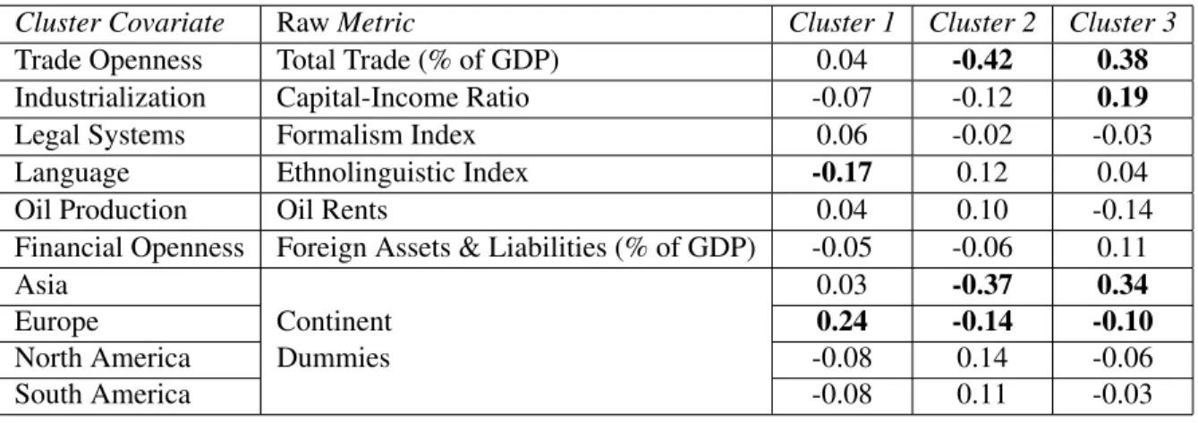
2.4.1 Cluster Covariates
The cluster covariates are country-specific variables which potentially inform business cycle
synchronization across countries by influencing the prior distribution on cluster membership. We
consider six variables: (1) the degree of trade openness, (2) financial integration, (3) the degree of
industrialization, (4) oil rents, (5) a formalism index, (6) an ethnolinguistic index, and (7) continent
dummies. The top panel of Table B.8 lists the sources for each cluster covariate as well as any
transformations made to the raw data.
The degree of trade openness of a country is measured as total trade as a percentage of its GDP
using data from Penn World Tables 8.0. A country with a high degree of trade openness is more
exposed to foreign demand and supply shocks, leading to a higher degree of synchronization with
its trading partners. However, economic theory also suggests that countries with a high degree of
trade openness may have more divergent cycles due to production specialization (Imbs, 2004). We
do not separate these channels, but rather examine how trade openness influences synchronization
inside of our different clusters of countries.
We measure financial openness as the sum of total foreign assets and total foreign liabilities
as a percentage of GDP, with data provided by Lane and Milesi-Ferretti (2007). Recent
theoreti-cal studies reached conflicting conclusions of how financial openness affects synchronization [See
![Table B.6: Estimates for the Transition Probability Parameters - Median posterior draws for the parameters governing the transition probabilities, p ji,t = Pr[s t = j|s t−1 = i, y U S t−1 ]](https://thumb-us.123doks.com/thumbv2/123dok_us/8308423.2200417/73.918.128.791.185.532/estimates-transition-probability-parameters-posterior-parameters-transition-probabilities.webp)