BAYESIAN PENALIZED METHODS FOR HIGH-DIMENSIONAL DATA
Zakaria S Khondker
A dissertation submitted to the faculty of the University of North Carolina at Chapel Hill in partial fulfillment of the requirements for the degree of Doctor of Philosophy in the Department of Biostatistics.
Chapel Hill 2013
Approved by:
c
2013
Zakaria S Khondker ALL RIGHTS RESERVED
ABSTRACT
ZAKARIA S KHONDKER: BAYESIAN PENALIZED METHODS FOR HIGH-DIMENSIONAL DATA
To my family who made it possible. Specially, to my wife Eema for so many reasons that I cannot list here. For five years, since I quit graduate school, Eema kept pushing me and finally succeeded in getting me back again. She made drastic lifestyle compromises and cutbacks, to live under the poverty line, with two children, on my meager income of a graduate research assistant. She dealt with my frustrations, stemming from having to unnecessarily abandon projects after significant progress and having to unnecessary rework and delays. To my children Bornali and Borneil, who had to compromise their playtime with their father and were understanding of my time constraints.
ACKNOWLEDGMENTS
TABLE OF CONTENTS
LIST OF TABLES . . . x
LIST OF FIGURES . . . xi
1 SHRINKAGE ESTIMATION IN THE LITERATURE . . . 1
1.1 Shrinkage of Mean Parameters for Univariate Response . . . 1
1.2 Shrinkage of Covariance Parameters . . . 3
1.2.1 Frequentist Methods . . . 3
1.2.2 Bayesian Non-Graph Theory Methods . . . 7
1.2.3 Bayesian Graph Theory Methods . . . 10
1.3 Multivariate Response Regression Model . . . 12
1.3.1 Traditional Estimation of Regression Coefficients . . . 14
1.3.2 Low Rank Estimation . . . 16
1.3.3 Low Rank Estimation Under Longitudinal Setting . . . 19
1.4 Motivating Examples . . . 21
1.5 Methods Background . . . 23
2 THE BAYESIAN COVARIANCE LASSO . . . 25
2.1 Introduction . . . 25
2.2 The General Method . . . 26
2.2.1 Proposed Priors . . . 26
2.2.2 Full Conditionals . . . 28
2.2.3 Proposed Sampling Scheme . . . 30
2.2.4 Credible Regions . . . 34
2.3 Simulation Study . . . 35
2.3.1 Criteria for comparison . . . 36
2.3.2 Results . . . 37
2.4 Application to Real Data . . . 38
2.5 Discussion . . . 44
3 BAYESIAN GENERALIZED LOW RANK REGRESSION . . . 54
3.1 Introduction . . . 54
3.2 Generalized Low Rank Regression Models . . . 57
3.2.1 Model Setup . . . 57
3.2.2 Low Rank Approximation . . . 60
3.2.4 Priors . . . 62
3.2.5 Posterior Computation . . . 63
3.2.6 Determining the Rank of B . . . 65
3.2.7 Thresholding . . . 67
3.3 Simulation Study . . . 68
3.3.1 Simulation Setup . . . 68
3.3.2 Results . . . 71
3.4 The Alzheimer’s Disease Neuroimaging Initiative . . . 74
3.4.1 Imaging Genetic Data . . . 74
3.4.2 Results . . . 76
3.5 Discussion . . . 78
4 BAYESIAN LONGITUDINAL LOW RANK REGRESSION . . . 89
4.1 Introduction . . . 89
4.2 The Alzheimer’s Disease Neuroimaging Initiative . . . 92
4.3 Methods . . . 94
4.3.1 Model Setup . . . 94
4.3.2 Priors . . . 96
4.3.3 Posterior Computation . . . 99
4.4 Simulation Study . . . 100
4.4.1 Simulation Setup . . . 100
4.4.2 Comparison of Results . . . 103
4.4.3 Results . . . 104
4.5 Application to ADNI Data . . . 105
4.5.1 Longitudinal Age Effect . . . 107
4.5.2 Regions of Interest . . . 108
4.5.3 SNPs . . . 109
4.6 Discussion . . . 110
5 CONCLUSION . . . 122
APPENDIX: DERIVATION OF CONDITIONALS . . . 124
LIST OF TABLES
1.1 Bayesian priors for mean parameter estimation . . . 4
2.1 Mean L1 losses (and standard deviations) for the different methods . . . 39
2.2 Mean L2 losses (and standard deviations) for the different methods . . . 40
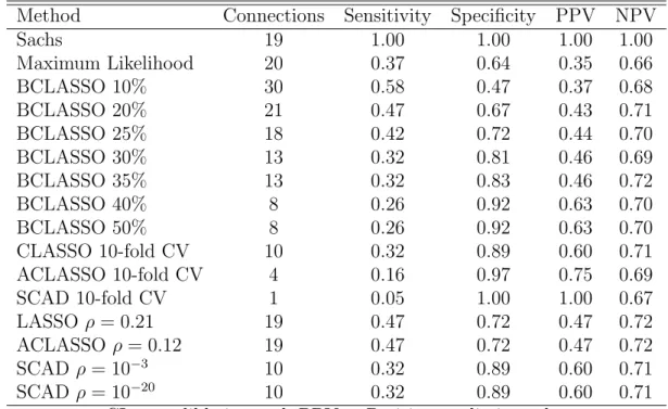
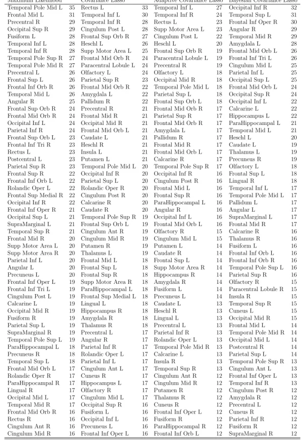
2.3 Mean matrix correlations (and standard deviations) for the different meth-ods . . . 41 2.4 Agreement of Methods with the Results from Sachs et al. (2003) . . . 52 2.5 ROIs With the Highest Number of Connections Picked by the Four Methods 53
3.1 Empirical comparison of GLRR3, GLRR5, LASSO, BLASSO and G-SMuRFS under Cases 1-5 based on the five selection criteria. The means and standard deviations of these criteria are also calculated and their standard deviations are presented in parentheses. Moreover, UN denotes the unstructuredB. . . 73 3.2 Ranked top SNPs based on the diagonal of BbinBbinT and columns ofU. . 79 3.3 Ranked top ROIs based on the diagonal of BbinT Bbin and columns of V. . 88
4.1 Empirical comparison of L2R2 and G-SMuRFS under Cases 1-4 based on the six selection criteria for moderate and extreme sparsity of B. The means and standard deviations of these criteria are also calculated and their standard deviations are presented in parentheses. . . 106 4.2 Top ROIs based onBT
binBbin, p-values of U, and magnitude of coefficients for model using SNPs from top 10 genes. . . 112 4.3 Top ROIs based onBbinBbinT , p-values of U, and magnitude of coefficients
for model using SNPs from top 45 genes. . . 113 4.4 Top SNPs based onBbinBbin0 , p-values ofU, and magnitude of coefficients
for model using SNPs from top 10 genes. . . 120 4.5 Top SNPs based onBbinBbin0 , p-values ofU, and magnitude of coefficients
for model using SNPs from top 45 genes. . . 121
LIST OF FIGURES
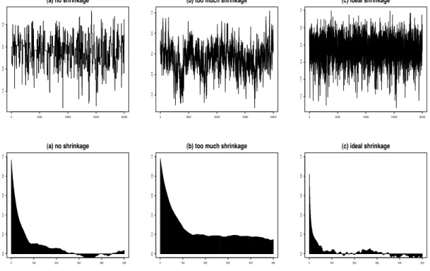
2.1 Trace plots (top row) and autocorrelation plots (bottom row) of θ12 for
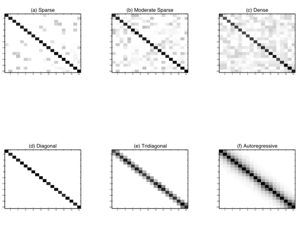
d= 5 and n = 10 showing the impact of variance tuning of the proposal density. . . 47 2.2 Image plots of the six types of precision matrices (Θ) considered in the
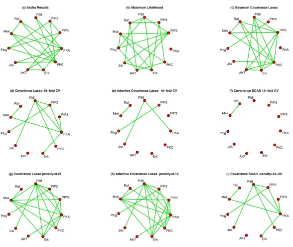
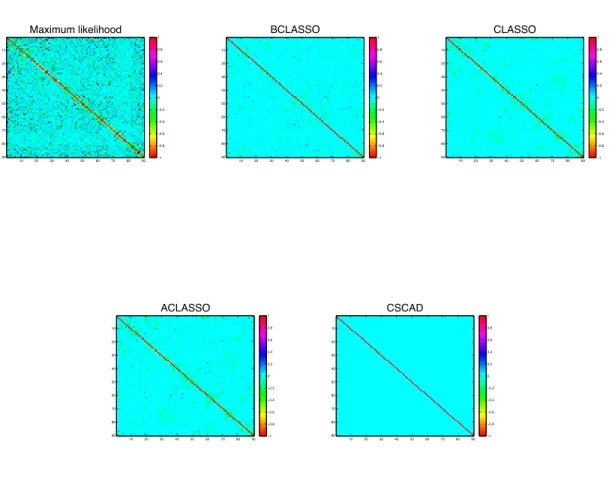
simulation study. The top 3 are unstructured and the bottom 3 are structured. . . 48 2.3 Networks for 11 proteins from Sachs et al. (2003) . . . 49 2.4 Image plots of the partial correlation matrices for 90 regions of 2-year old
children’ brains using the five different methods . . . 50 2.5 Networks for 90 regions of 2-year old children’ brains using the different
methods . . . 51
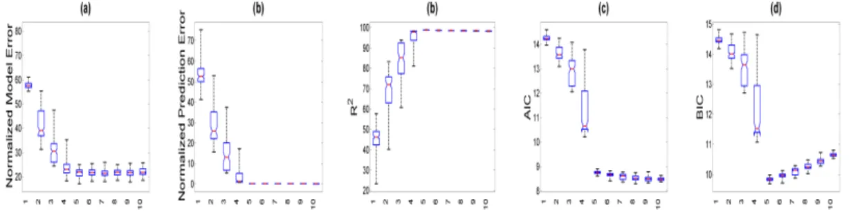
3.1 Simulation results: the box plots of five selection criteria including MEN( ˆB, B), PEN(Yb,Y),R2(Yb,Y), AIC, and BIC against rankr from the left to the
right based on 100 simulated data sets simulated from model (3.4) with (n, p, d) = (100,200,100) and the true rank r0 = 5. . . 81
3.2 Simulation results: comparisons of true B image and estimated true B images by using LASSO, BLASSO, G-SMuRFS, GLRR3, and GLRR5 under five different scenarios. MEN(B,B) and BIC were calculated forˆ each estimated ˆB. The sample size isn = 1000. Columns 1-5 correspond to Cases 1-5, respectively. The true ranks of B under Cases 1-5 are, respectively, 2,5,5,100 and 100. The top row contains trueB maps under Cases 1-5 and rows 2-6 correspond to the estimated ˆB under LASSO, Bayesian LASSO, G-SMuRFS, GLRR3, and GLRR5, respectively. For simplicity, only the first 100 rows and 100 columns of B were presented. Moreover, all plots in the same column are on the same scale. . . 82 3.3 Comparisons of GLRR3, GLRR5, and LASSO under Cases 1-5: mean
3.4 Results of ADNI data: the posterior estimate of ˆB matrix after thresh-olding out elements whose p− values are greater than 0.001 (left panel), BbinT Bbin (middle panel) and BbinBbinT (right panel) in the first row; and the −log10p−value matrices corresponding to B (left panel), U (middle panel), andV (right panel) in the second row. . . 84 3.5 Results of ADNI data: the top 20 ROIs based onBT
binBbin and the first 3 columns of V. The sizes of the dots represent the rank of the ROIs. . . . 85 3.6 Results of ADNI data: at a -log10(p) significance level greater than 6.3,
the top row depicts the locations of ROIs that are correlated with SNPs rs10792821 (PICALM), rs9791189 (NEDD9), rs9376660 (LOC651924), rs17310467 (PRNP), rs4933497 (CH25H), respectively; the bottom row shows the ROIs correlated with SNPs rs1927976 (DAPK1), rs1411290 (SORCS1), rs406322 (IL33), rs1018374 (NEDD9), and rs439401 (APOE). The sizes of the dots represent the absolute magnitudes of the regression coefficients. . . 86 3.7 Heatmaps of coefficients between SNPs and ROIs on the left (left panel)
and right (right panel) hemispheres. Coefficients with −log10(p) -value smaller than 6.3 are set to 0. . . 87
4.1 Simulation results: Mean ROC curves from L2R2 (red line for B, black line for Γ), and G-SMuRFS (blue line for B, black dashed line for Γ) based on 100 samples of size n = 100 each. Top row for moderately sparse B and bottom row for extremely sparse B, while Γ remains the same in both scinarios. . . 114 4.2 Simulation results: Splines for standardized volumes of selected ROIs
(from left to right, respectively, ROIs 1, 4, 7 and 8) from single sam-ple. Black lines are generated by true G, red lines by estimates from G-SMuRFS, and blue by estimates from LGLRR. Top row is based on G when B is moderately sparse and bottom row is based on G when B is extremely sparse. L2R2 did a decent job in estimating the true splines while G-SMuRFS can be off for some ROIs. . . 115 4.3 Simulation results: Image plots of the low-rank componentB from single
sample. True B on the left, G-SMuRFS in the middle, and L2R2 on the right. Top row is moderately sparse B and bottom row is extremely sparseB. For moderatly sparseB G-SMuRFS may pick up too much noise.116 4.4 Splines functions: all the ROIs on the left, selected ROIs with declining
volumes in the middle, selected ROIs with increasing volumes on the right. Top row from the model using SNPs from top 10 genes, bottom row from the model using SNPs from top 45 genes. . . 117
4.5 Data analysis results from SNPs in the top 10 genes: Top panel (a) left-LD correlation of selected SNPs from top 10 genes in AlzGene database (b) middle- ROI network from binary B (c) right- SNP network from binary B. Bottom panel (d) left- age by SNP interaction part of sparse B after thresholding with negative log10(p) > 10, (e) middle- negative log10(p) of U (f) right- negative log10(p) of V. . . 118
4.6 Data analysis results from SNPs in the top 45 genes: Top panel (a) left-LD correlation of selected SNPs from top 45 genes in AlzGene database (b) middle- ROI network from binary B (c) right- SNP network from binary B. Bottom panel (d) left- age by SNP interaction part of sparse B after thresholding with negative log10(p) > 10, (e) middle- negative
CHAPTER 1
SHRINKAGE ESTIMATION IN THE LITERATURE
The emergence of high-dimensional data has posed tremendous challenges to the traditional approches to modeling and estimation, in some cases, rendering traditional modeling approaches obsolete. As a remedy the idea of penalized mehods are gaining popularity among the statistical community. Here we discuss the literature of early and latest approches approaches in univariate and multivariate context. Our primary focus is on multivariate approaches since it it most relevant to our problem.
1.1 Shrinkage of Mean Parameters for Univariate Response
The later approaches adopted shrinkage−shrinking the parameters to achieve stabil-ity and improve performance. The most popular among them are the L1 and L2 priors
and their variants. The L2 priors (penalties) tend to shrink the regression coefficients
to achieve stability; it forces the coefficients of highly correlated covariates towards each other by inflating the diagonals of the XTX, where X is the matrix of covariates. The most common example of L2 priors are normal (Ridge regression) and Cauchy priors.
Recently there has been a surge in black hole priors− priors that create a singular-ity at the origin with a black hole around. The prior forces the maximum aposteriori (MAP) estimates of the smaller coefficients to singularity without creating discontinuity to perform simultaneous variable selection and estimation. The most common of them are lasso (Tibshirani, 1996), adaptive lasso (Zou, 2006), smoothly clipped absolute de-viation (Fan and Li, 2001), and double Pareto (Armagan et al., 2011). Some hybrids and other variants of these priors include grouped lasso, fused lasso, elastic net, etc. Rothman et al. (2010) proposed simultaneous estimation of sparse coefficient matrix and sparse covariance matrix to improve on estimation error under L1 penalty. Their
approach does not take advantage of the potential correlation among the coefficients.
The penalized methods estimates the coefficients by minimizing the residual sum of squares (RSS) with a constraint, that is, minimizing ||Y −Xβ||2+g(β), where g(β) is
some penalty function. A popular general choice is g(β) = λPp
j=1|βj|
Bayesian shrinkage regression methods achieve regularization through shrinkage in-duced by priors. Summarized in tabel 1.1 are the commonly used scaled mixture of normal priors which lead to heavy-tailed priors with a peak around the origin (Carvalho and Scott, 2009a; Armagan et al., 2011; Park and Casella, 2008; Kyung et al., 2010).
1.2 Shrinkage of Covariance Parameters
In-depth theoretical studies of the sample (empirical) covariance matrixShave shown that without regularization, the sample covariance matrix performs poorly in high di-mensional settings, hence stimulating research on alternative estimators. When the dimension of the matrix is large, the largest eigenvalue can be very large compared to the smallest eigenvalue, resulting in a large condition number and unstable estima-tors for the precision matrix S−1. In practice, when n is relatively small compared to the dimension d, the S matrix approaches singularity, therefore leading to unreliable estimates for the precision matrix S−1. In many cases, such a situation may lead to
near-zero eigenvalues for S. The problem is even more serious for high-dimensional data (when n < d) derived from structural and functional magnetic resonance imaging where a few dozen subjects are scanned with each scan having thousands of voxels or hundreds of regions of interest, gene arrays where few dozen or hundred samples are arrayed each array containing several hundred to several thousand genes (Davidson and Levin, 2005), spectroscopy, climate studies and many other applications are just a few examples. In this case, S has a maximum rank ofn which is smaller than its dimension d, and therefore S is singular.
1.2.1 Frequentist Methods
In the frequentist framework, significant work has been done on model selection and precision (covariance) matrix estimation in Gaussian models (Banerjee et al., 2007;
T able 1.1: Ba y esian priors for mean pa rameter estimation Mo del Prior on β h yp er-prior h yp er-h yp er-prior NJ βj ∼ N (0 ,σ 2 ψ j ) π ( ψj ) ∝
1 ψj
NE βj ∼ N (0 ,σ 2 ψ j ) ψj ∼ Exp(
λ ) 2
,λ > 0 NIGam βj ψj ∼ N (0 ,σ 2 ψ j ) ψj ∼ IGgam( a0 ,a 0 b
2 )0
NG βj ψj ∼ N (0 ,σ 2 ψ j ) ψj ∼ Gamma( a0 ,b
2 )0
NEG βj ψj ∼ N (0 ,σ 2 ψ j ) ψj ∼ Exp(
λj 2
) λj ∼ Gamma( a0 ,b0 ) LASSO βj ψj ∼ N (0 ,σ 2 ψ j ) ψj ∼ Exp( λ
2 ) 2
λ 2 ∼ Gamma( a0 ,b 0 ) HS βj ∼ N (0 ,ψ j ) ψj ∼ C + (0 ,τ ) τ ∼ C + (0 ,σ ) gDP βj ∼ N (0 ,ψ j ) ψj ∼ Exp( λ
2 ) 2
Friedman et al., 2008a; Fan et al., 2009; Drton and Perlman, 2004). The original pa-per by Dempster (1972) introduced the idea of shrinkage estimation which forces some elements of the precision matrix to be zero. In its infancy, the methods for shrinkage estimation involved two steps: (i) identify the “correct” model by determining which el-ements are zero; (ii) estimate the parameters for the non-zero elel-ements. Edwards (2000) has discussed some standard approaches for identifying the model such as greedy step-wise forward-selection and backward-elimination procedures, achieved through hypothe-sis testing. Drton and Perlman (2004) proposed a conservative simultaneous confidence interval to select a model in a single step as an improvement.
Banerjee et al. (2007) proposed block coordinate descent algorithm which can be interpreted as recursive l1-norm penalized regression. Suppose y ∼ N(µ,Σ), S =
Pn
i=1(yi−µ)(yi−µ)
T and Ω = Σ−1 then the estimate takes the form
ˆ
Ω = arg max
Ω0 log det Ω−tr(SΩ)−λ||Ω||1; (1.1)
wherestands for positive definite, ||Ω||1 denotes the sum of the absolute values of the
elements of the positive definite matrix Ω, and λ is the penalty scalar (proxy for the number of nonzero elements in the matrix). When S 0, MLE of Σ can be obtained by setting λ= 0, however Σ is not invertible for n < p.
Let W = ˆΣ be an estimate of Σ, the dual of their sparse maximum likelihood problem is
ˆ
Σ−1 = max{log detW :||W −S||∞≤λ}. (1.2)
They choose the penalty parameter as a function of α, the probability of zero element of Σ falsely estimated as non-zero. Their plan is to optimize over one rwo and column of the variable matrix W at a time and repeatedly sweep through all columns until
convergence. In other words, partition W and S as:
W =
W−kk wk wTk wkk
and S =
S−kk sk sTk skk
, (1.3)
where θkk is the kth diagonal element of Θ,θk = (θk1, . . . , θk,k−1, θk,k+1, . . . , θkd)T is the vector of all off-diagonal elements of thekth column, and Θ−kk is the (d−1)×(d−1) matrix of all the remaining elements, i.e., the matrix resulting from deleting thekth row and kth column from Θ. Then the algorithm proceeds as follows:
1. Initialize W(0) =S+λI, forj = 1. . . p letW(j−1)denote the current iterate. Solve
the quadratic program ˆ
y= arg miny{yT(W
(j−1)
−(jj))
(−1)y :||y−s
j||∞ ≤λ}.
2. Update rule: W(j) isW(j−1) with w
j replaced by ˆy. 3. Let ˆW(0) =W(p).
4. Check convergence by tr{( ˆW(0))−1S} − p+ λ||( ˆW(0))−1||1 ≤ , where is the
convergence criterion.
Friedman et al. (2008b) used similar partitioning as Banerjee et al. (2007) and showed that minimizing (1.1) is equivalent to minimizing: minθ||W
1/2
11 θ−
1
2W
−(1/2)
11 s12||2+ρ||θ||1
Where ˆθis the solution to the above lasso problem (3). That is they use lasso to estimate
ˆ
θ = arg min||W111/2θ− 1
2W
−(1/2)
11 s12||2 +ρ||θ||1 (1.4)
Their covariance LASSO algorithm has the following 3 steps:
1. Start with W =S+ρI. The diagonal of W remains unchanged in what follows.
productsW11ands12. This gives ap−1 vector solution ˆθ. Fill in the corresponding
row and column of W using w= 2W11θ.ˆ
3. Continue until convergence.
Fan et al. (2009) solved the following equation for sparse matrix under the penalized likelihood framework.
max
Ω∈Sp
log det Ω−tr( ˆΣΩ)−
p
X
i=1
p
X
j=1
pλij(|ωij|), (1.5)
whereωij is the (i, j)th element of Ω,λij is the tuning parameter andp(.) is the generic penalty function on each element.
Sch¨afer and Strimmer (2005) minimized the MSE compromising between bias and variance. If ˆΘ is the unrestricted estimate and ˜Θ the restricted estimate from a reduced model then the optimal estimate is ˆΘ∗ =λΘ + (1˜ −λ) ˆΘ for a suitable shrinkage intensity λ ∈ [0,1]. The value of λ is determined by minimizing the risk R(λ) = E(L(λ)) = E(Pp
i=1(ˆθ
∗
i −θi)2. They minimized this analytically to obtain the optimal valueλ∗ as a function of variances of ˆΘ and ˜Θ, their covariances and bias respectively, which is unique and always exist. For practical purpose they replace those variances, covariances and biases by their unbiased sample counterparts to obtain ˆλ∗. For finite samples the value might be negative or exceed unity, in which case they truncate it to zero or one.
1.2.2 Bayesian Non-Graph Theory Methods
Bayesian covariance estimation followed two major paths. The non-graph theory methods disregard the underlying graphical structures and perform shrinkage via pri-ors on the elements, eigenvalues, and decompositions of the matrix. The graph theory methods rely assuming particular graphical structure and hyper-inverse Wishart priors conditional on the graph. Among Bayesian shrinkage methods, Yang and Berger (2007)
used reference priors on the eigenvalues of the covariance matrix to regularize the eigen structure.
Smith and Kohn (2002) decomposed Σ−1 = Ω = BDBT where B is a lower trian-gular matrix with 1’s on the diagonal and D is a diagonal matrix. They introduced an indicator matrix γ where bij = 0 iff γij = 0 bij 6= 0 iff γij = 1, which ensures that the lower triangular elements of B can be 0 with positive probability. For a given γ, some often the lower-triangular elements of B will be zero. For the unconstrained elements of B, denotedBγ, they used fractional prior asp(Bγ|γ, D)∝p(e|B, D, γ)1/n. The elements ofγ are taken independent a priori, withp(γij = 1|ω) =ω, which implies that there will p(p−1)ω/2 nonzero elements in B. They assumed uniform [0,1] prior for ω.
Fr¨uhwirth-Schnatter and T¨uchler (2008) used Cholesky decomposition on hierarchi-cal linear mixed models to identify zeros on the covariance matrix Σ = CCT, where C
is a lower triangular matrix (Smith and Kohn (2002) decomposed Σ−1). This approach
Barnard et al. (2000) used separation strategy as Σ = diag(S) R diag(S) where S is vector of the standard deviations andR is the correlation matrix. There is a prac-tical motivation for this separation since most practitioners think in terms of standard deviations and correlations. They assume S ∼ N(ξ,Λ), alternative would be to choose independent scaled inverted chi-squared distributions for each of the variances. They assume R independent of S, {rij, i 6=j} are a priori exchangeable, and priors are dif-fuse to reflect week prior knowledge about R. They explored two extreme cases- (1) marginally uniform, which can be obtained from the commonly used inverse-Wishart distribution for Σ, and (2) jointly uniform prior for rij.
Wong et al. (2003) decomposed Σ−1 = Ω =T CTT where T is a diagonal matrix such thatTi is the inverse of the partial standard deviation ofyit and C is a correlation matrix withCii= 1 andCij =−ρij the partial correlation coefficients. They put noninformative gamma priors on{Ti, i= 1, ..., p} assuming Ti i.i.d. and independent of the elements of C, p(Ti)∝p(Ωii)ddTΩii
i ∝ T
2α−1
i e
−βT2
i. Their sampling scheme used MCMC based on the
following Metropolis-Hastings algorithm: q(Ti|Y, T(−i), C) and q(dCij|Y, T, C(−ii)). The
Ti, are generated one at a time using a Gaussian proposal. The Cij are generated one at a time using a Metropolis-Hastings proposal that allows Cij to be identically zero, and that uses a Gaussian proposal for the continuous part of the conditional density.
Chen and Dunson (2003) used modified Cholesky decomposition Σ = LLT = ΛΓΓTΛ
where Γ =diag(γ1, ..., γp) then the random effects model becomesyi =Xiα+ZiLbi+i. In their first paper they applied the method to linear mixed model and in the second paper they applied to logistic regression.
Huang et al. (2006) proposed nonparametric method for identifying parsimony in es-timating covariance matrix using modified Cholesky decomposition. If cov(y) = Σ and
=T y with cov() = diag(σ2
1, ..., σn2) =D then Σ
−1 =TTD−1T and the likelihood
be-comes−2l(Σ, y) = Pn
t=1log(σt2) +
Pn
t=1
t
σ2
t. Thus the modified Cholesky decomposition
provides a parameterization of the covariance matrix with unconstrained parameters and tramsfers the difficult task of modeling a covariance matrix to that of variable selection in the sequence of regression yt =
Pt−1
j=1φtjyj +t.
Their penalized likelihood estimator was derived as the Bayes posterior mode under independent diffuse priors. The algorithm amounts to applying a similar regression algorithm repeatedly to the rows of the Cholesky factor T. The authors claimed this method to be better than smoothing when T is sparse instead of being smooth.
1.2.3 Bayesian Graph Theory Methods
Bayesian graph theory methods exploit decomposability and use hyper-inverse Wishart priors to sample from the marginal.
Guidici and Green (1999) used HIW priors on the precision matrix conditional on decomposable graphs for Bayesian model determination in Gaussian graphical mod-els. They introduced hierarchical Bayesian Gaussian graphical models and designed reversible jump Markov chain Monte Carlo (MCMC) algorithm for structural and quan-titative learning using local computations.
LetG= (V, E) be an undirectedgraphwithvertexsetV ofvelements andedge−set E. If there is an edge (a, b) ∈ E then the vertices a and b are called neighbors in G and if all vertices are connected the graph is complete. A complete subgraph which is not contained in another complete subgraph is a clique. Subgraphs (A, B, C) of G forms a decomposition of G if any path from A to B goes through C. In other words if V =A∪B, C =A∩B is complete, and the all paths from A and B are through C only then (A, B, C) form a decomposition and C is said to be separator. A sequence of subgraphs that cannot be further decomposed are the prime components of a graph and a graph is decomposible only if all its prime components are complete.
Carvalho and Scott (2009b) developed Wishart g-prior, a default version of the hyper-inverse Wishart prior for restricted covariance matrices and showed how it corresponds to the implied fractional prior for selecting a graph using fractional Bayes factors. Then they applied a class of priors that automatically handles the problem of multiple hy-pothesis testing. They demonstrated that the combined use of a multiplicity-correction prior on graphs and fractional Bayes factors for computing marginal likelihoods yields better performance.
How well these graphical methods do when there is no prior knowledge of the un-derlying graph structure is not studied yet. Furthermore, these methods don’t work for any type of graph. Existing non-graph theory Bayesian methods rely on priors on the
elements arising from some sort of decomposition of the precision (covariance) matrix, which do not readily translate to any recognizable priors on the elements of the precision (covariance) matrix itself. Furthermore, most of those methods are based on sampling the elements of the matrix one at a time which is not efficient and not attractive for high-dimensional data, especially when d is large. Specifically, these methods pick a single element at a time, find an appropriate boundary that yields a positive definite matrix, and then draw a sample of this element. Drawing one element at a time is inefficient, and coupled with the additional computational complexities in computing boundaries for the elements; these methods are not suitable for high-dimensional matrices. Graphs theory methods, however, does not work for all graphical structures limiting their use. We will focus on non-graph theory approach.
1.3 Multivariate Response Regression Model
The model for multivariate regression is
Y =XB+, (1.6)
where Y is the n×d matrix of responses, X is the n ×p matrix of predictors, B is the p×d matrix of regression coefficients, and is the n×d matrix of random errors. Alternatively, we can write
yik = p
X
j=1
xijβjk+ik,
where i is the subject index (i = 1, . . . n), j is the predictor index (j = 1, . . . p), and k is the response index (k = 1, . . . d). Error terms ik and ik0,(k 6= k0) represent the
different responses within a subject (e.g., fMRI signals from regions k and k0 of subject i) and are likely to be correlated, while eik and ei0k,(i6=i0) represent the same response
The emergence of high-dimensional data in genomics, imaging, econometrics, chemo-metrics and other quantitative area has presented us with a large number of predictors along with a large number of response variables that calls for simultaneous variable selec-tion and estimaselec-tion of both the mean and covariance parameters. Tradiselec-tionally, subset selection was used for variable selection and least squares was used for estimation when presented with large number of predictors. However, the subset selection approach is unstable due to discontinuity of the process. When either the dimensiond of the covari-ance matrix or the number of predictorspis larger than the sample size the model is not identifiable, leading to failure of the traditional methods like least squares or maximum likelihood. Forp > nthe subset selection method can be unstable because the procedure is not continuous (Breiman, 1996). Even when the sample size is larger than both the dimension of the covariance matrix and the number of predictors traditional methods are stable only when both d
n and p
n are reasonably small. When d
n < 1, but not small enough, the condition numbers of the maximum likelihood estimatorS of the covariance matrix can be unusually large leading to unstable estimators for the precision matrix (Khondker et al., 2011). When np <1, but not small enough, the condition numbers of the matrix XTX, where X is the covariate matrix, can be unusually large leading to
unstable least squares estimators for the mean parameters.
Best single-model variable selection is inherently unstable and Bayesian model aver-aging provides a robust prediction remedy. Under squared error loss optimal prediction takes the form of Bayes model averaging (see Brown et al. (2002) and references therein). The shrinkage approaches for estimation of B can be divided into two major groups -(1) without decomposition and (2) via decomposiotn.
1.3.1 Traditional Estimation of Regression Coefficients
The curse of dimensionality boils down to dealing with too many parameters than the sample size reasonably permits. When dimension is larger than the sample size the model is unidentifiable and all the parameters are not estimable. Even when the dimension is smaller than the sample size but dimension to sample size ratio is not small enough or there is colinearity among the predictors the estimators are unstable. The early approaches involved separation approach− variable selection to reduce dimension and then parameter estimation. While subset selection techniques were used in variable selection, estimation was typically done by least squares regression. However, the subset selection approach is unstable due to discontinuity of the process; so is the best single-model variable selection (Breiman, 1996). Bayesian single-model averaging provides a robust prediction remedy regarding stability; under squared error loss optimal prediction takes the form of Bayes model averaging. Brown et al. (2002) introduced Bayes model aver-aging incorporating variable selection allowing for fast computation for dimensions up to several hundreds.
Another approach is shrinkage− shrinking the parameters to achieve stability and improve performance. The most popular among them are the L1 and L2 priors and
their variants. The L2 priors (penalties) tend to shrink the regression coefficients to
achieve stability; it forces the coefficients of highly correlated covariates towards each other by inflating the diagonals of the XTX, where X is the matrix of covariates. The
most common example of L2 priors are normal (Ridge regression) and Cauchy priors.
are lasso (Tibshirani, 1996), adaptive lasso (Zou, 2006), smoothly clipped absolute de-viation (Fan and Li, 2001), and double Pareto (Armagan et al., 2011). Some hybrids and other variants of these priors include grouped lasso, fused lasso, elastic net, etc. Rothman et al. (2010) proposed simultaneous estimation of sparse coefficient matrix and sparse covariance matrix to improve on estimation error under L1 penalty. Their
approach does not take advantage of the potential correlation among the coefficients.
Breiman and Friedman (1997) considered the problem of predicting several response variables from the same set of explanatory variables and showed that even when the random error terms eik and eik0 are independent for different responses the responses
yik and yik0 of a sample i can be correlated due to their dependence on the same
pre-dictor set Xi. They introduced shrinkage estimation called ”Cards and Whey” that predicts the multivariate response with an optimal linear combination of the ordinary least squares predictors method to take advantage of the correlation in the responses arising from shared random predictors as well as correlated errors. This is a multivariate generalization of proportional shrinkage based on cross-validation and derives its power by shrinking in the right co-ordinate system (canonical co-ordinates).
Rothman et al. (2010) proposed simultaneous estimation of sparse mean parame-ters and the covariance matrix called multivariate regression with covariance estimation (MRCE). They improve prediction in the multivariate regression problem while allowing for interpretable models in terms of the predictors. They reduced the number of param-eters using theL−1 penalties on both the mean parameterB and covariance parameter Ω in optimizing the likelihood. MRCE assumes the predictors are not random and fo-cused on the conditional distribution of Y givenX, althout, the formulas would be the same with random predictors. Unlike in the Curds and Whey framework, the MRCE assumes that correlation of the response variables arises only from the correlation in the
errors.
1.3.2 Low Rank Estimation
Principal component analysis (PCA) is arguably the most widely used statistical tool for data analysis and dimensionality reduction for multivariate response. A num-ber of natural approaches to robustifying PCA have been explored and proposed in the literature over several decades including influence function techniques, multivariate trimming, alternating minimization, random sampling techniques, etc. (Cand´es et al., 2009; Jolliffe, 2002). A convenient approach is via decompose the data matrix into a diagonal matrix of singular values ∆ and two unitary matrices U and V, that is
Y =U∆V = r
X
l=1
δlulvTl . (1.7)
A common convention is to list the singular values in descending order. The rank is reduced by minimizing the dimension r of ∆.
Cand´es et al. (2009) applied robust principal component analysis when response is a superposition of a low-rank component and a sparse component (Y = Y0 +S0) to
recover the two components individually. Their method Principal Component Pursuit is used to recover the low rank componentY0 =U∆VT =
Pr
l=1δlulvTl .
correlations. In quantitative trait studies problems arise when high-dimensional re-sponse sets such as fMRI signals or volumes of each voxel in the brain are predicted by high-dimensional covariate sets such as gene expression or SNPs. Genes or SNPs may co-conspire, working in unison, to produce similar patterns of fMRI signals in the brain. In such situations regression coefficients are both vertically and horizontally correlated with rank smaller than dimension. For example, Alzheimer’s Disease Neuroimaging Initiative (ADNI) collects clinical, imaging, genetic, and biospecimen data on elderly controls, mildly cognitive impaired, and Alzheimer’s patients. To study the impact of SNPs on the volumes of certain regions of interest one has to expect some common pattern of correlation among the regression coefficients. The responses and predictors may be associated through fewer channels than the dimensions of the coefficient matrix leading to a reduced rank of the mean parameterB.
The relationship among correlated responses and predictors may be exploited by dimension reduction via reduced rank decomposition of the regression parameters to greatly reduce the number of parameters and facilitate efficient estimation of the coef-ficient matrix. This factorization has started to receive more attention in recent years. Several authors have explored the decomposition of the response matrix Y (see Ding et al. (2011) and the references therein). Others took the latent model approach to re-strict the rank of the coefficient matrix (Izenman (1975), Reinsel and Velu (1998)) and sparsity-inducing regularization techniques to reduce the number of parameters (Tib-shirani (1996), Turlach et al. (2005), Peng et al. (2010)). Chen et al. (2012) has used singular value decomposition of the coefficient matrixB withL1 penalty on the singular
vectorsU andV and computed the posterior modes for orthogonal design matrix. There method, however, is limited to orthogonal design matrix where columns of X must be independent. We relax the assumption to remove the orthonormality of U and V and allow correlated covariates as the regression coefficients are likely to be correlated both
ways. The coefficients in each row can be correlated as they are the effect of the same covariate on different responses for a particular subject. Moreover, the coefficients in each column can be correlated as they are the effect of different covariates on the same response for a particular subject. Our approach exploits this two-way correlation struc-ture in cases where regressors can be correlated and random.
Breiman and Friedman (1997) introduced shrinkage estimation called Cards and Whey (C&W) method to improve on prediction error when the same set of predictors is used for multivariate response. They showed that even when the random error terms eik and eik0 are independent for different responses the responses yik and yik0 of a sample
ican be correlated due to their dependence on the same set of predictorsXi. The C&W linear predictor has the form ˜Y = ˆYOLSM, where M is a d×d shrinkage matrix esti-mated from the data to exploit correlation in the responses arising from shared random predictors.
Ding et al. (2011) extended the idea in Bayesian framework and introduced a rank recovery mechanism; their low rank component is modeled as Y0 = U(Z∆)VT =
Pr
l=1δlzlulvlT, where Z is diagonals matrix with zl ∈ {0,1}. They claimed that restric-tions on U, V, and ∆ comes at a greater computational cost without any remarkable benefit. Relaxing the orthonormality assumptions of U and V and non-negativity as-sumption on ∆, that allows for a more flexible prior specification, they used normal priors for ul, vl and δl to achieve shrinkage. A binomial prior is used for zl, which is introduced for rank learning.
importance, and each layer provides a distinct channel relating the responses to the pre-dictors, which parsimoniously reveals the structure imposed by (1.7). They sought to seek a ˆB with sparse SVD structure in the vicinity of some initial consistent estimator ˜B by decomposing the rank-rproblem intorparallel sparse unit-rank regression problems, by forming r ”exclusive layers”.
None of the existing approches address the simultaneous estimation of high- dimen-sional mean parmeter matrix and high- dimendimen-sional covariance matrix.
1.3.3 Low Rank Estimation Under Longitudinal Setting
Many longitudinal biomedical studies, such as genomics and neuroimaging, repeat-edly collect a large number of responses and covariates from a small set of subjects and focus on establishing associations among them. For instance, in imaging genetics, various imaging measures, such as volumes of regions of interest (ROIs), are repeatedly measured and may be predicted by high-dimensional covariate vectors, such as single nucleotide polymorphisms (SNPs) or gene expressions. These imaging measures can serve as important endotraits that may ultimately lead to discoveries of genes for some complex mental and neurological disorders, such as schizophrenia, since imaging data provides the most effective measures of brain structure and function (Scharinger et al., 2010; Paus, 2010; Peper et al., 2007; Chiang et al., 2011b,a). This motivates us to develop a longitudinal low rank regression model for the analysis of longitudinal high-dimensional responses and covariates.
Modeling longitudinal high-dimensional covariates and responses involve four chal-lenges (i) a large number of regression coefficients, (ii) spatial correlation, (iii) temporal correlation, and (iv) multicollinearity among predictors. When the dimension of re-sponses and the number of covariates, which are denoted by d and p, respectively, are
even moderately high, fitting a multivariate linear model usually requires estimating a d×p matrix of regression coefficients, whose number pd can be much larger than the sample size. At each given time, accounting for complicated spatial correlation among multiple responses is important for improving prediction accuracy of multivariate analy-sis (Breiman and Friedman, 1997). Accounting for temporal correlation is important for both prediction and estimation accuracy. Moreover, the collinearity among genetic pre-dictors can cause issues of over-fitting and model misidentification (Fan and Lv, 2010).
Under the cross-sectional settings, several approaches explored new methods for high-dimensional responses and covariates. Breiman and Friedman (1997) introduced a Cards and Whey (C&W) to improve prediction error by accounting for correlations among the response variables when both pand d are moderate compared to the sample size. Peng et al. (2010) proposed a variant of the elastic net to enforce sparsity in the high-dimensional regression coefficient matrix, but they did not account for correlations among responses. Rothman et al. (2010) proposed a simultaneous estimation of a sparse coefficient matrix and a sparse covariance matrix to improve on estimation error under the L1 penalty. Vounou et al. (2010) considered the singular value decomposition of the
coefficient matrix and used the LASSO-type penalty on both the left and right singular vectors to ensure its sparse structure. They, however, do not model longitudinal data and do not provide a standard inference tool (e.g., standard error) on the nonzero com-ponents of the left and right singular vectors or the coefficient matrix.
regression to examine the association between genetic markers and longitudinal neu-roimaging phenotypes. However, their multi-task regression model considered subjects with the same number of repeated measures and ignore spatial-temporal correlations of imaging phenotypes, and thus it leads to loss of statistical power in detecting gene-imaging associations. Vounou et al. (2011) and Silver et al. (2012) proposed various sparse reduced-rank regression models by using penalized regression methods for the detection of genetic associations with longitudinal phenotypes. They, however, ignore the spatio-temporal correlations of longitudinal phenotypes, which are important for both estimation and prediction accuracy. Moreover, none of them explore the gene and time interaction, which can reveal important genetic traits altering time affects on longitudinal phenotypes.
1.4 Motivating Examples
Consider the challenges in the analysis of genetic and imaging data collected by the NIH ADNI. The NIH ADNI is an ongoing public-private initiative to test whether ge-netic, clinical, functional and structural neuroimaging data can be combined to measure the progression of mild cognitive impairment (MCI) and early Alzheimer’s disease (AD) . ADNI initiative is recruiting study subjects over 50 sites across the United States and Canada. The genetic and clinical data along with corresponding structural brain MRI data from baseline and follow-up were obtained from the ADNI publicly available database (http://adni.loni.ucla.edu/). Our interest is to perform genome-wide searches for establishing the association between the SNPs collected on top genes reported by Alz-Gen (http://www.alzgene.org/) and the brain volumes of 93 regions of interest (ROIs), while accounting for other time-varying covariates, such as age, and baseline covariates, such as gender, as well as spatiotemporal correlation among responses. By using the Bayesian GLRR for repeated measures data, we can easily carry out formal statistical inferences,such as the identification of significant SNPs or SNPs that interact with aging
on the differences among all 93 ROI volumes between AD and normal controls.
The MRI data was collected across a variety of 1.5 Tesla MRI scanners with indi-vidualized protocols for each scanner. To obtain standard T1-weighted images volumet-ric 3-dimensional sagittal MPRAGE or equivalent protocols with varying resolutions were used. The typical protocol included: inversion time (TI) = 1000 ms, repeti-tion time (TR) = 2400 ms, flip angle = 8o, and field of view (FOV) = 24 cm with a 256 ×256 × 170 acquisition matrix in the x−, y−, and z−dimensions yielding a voxel size of 1.25×1.26×1.2 mm3. Standard steps including anterior commissure and
posterior commissure correction, skull-stripping, cerebellum removing, intensity inho-mogeneity correction, segmentation and registration (Shen and Davatzikos, 2004) were used to preprocessed the MRI data. We then carried out automatic regional labeling by labeling the template and by transferring the labels following the deformable regis-tration of subject images. After labeling 93 ROIs, we were able to compute volumes for each of these ROIs for each subject.
We also performed quality control on this initial set of genotypes. In order to im-pute the missing genotypes in our sample, we used MACH4 version 1.0.16 with default parameters to infer the haplotype phase. We also included the APOE-4 variant, coded
as the number of observed 4 variants. We dropped SNPs with more than 5% missing
values and imputed the mode for the missing SNP for the remaining. In the final quality controlled genotype data, we dropped the SNPs with minor allele frequency smaller than 0.1 and Hardy-Weinberg p-value <10−6.
The data is multivariate whose covariance needs to be estimated in order to obtain a more precise estimate for the regression coefficients and build nework among the regions of interest. The covariates are hig-dimensional deserving special techniques for fitting feasible regression models. The responses are measureed repeatedly calling for accomodating speciotemporal correlation as well as age effect on response as well as genotype-phenotype relationship. We developed a series of three papaers to address these issues.
1.5 Methods Background
Our first paper introduces a genaralized double-gamma prior that can be reduced to commonly used frequentist methods. Then we develop a Bayesian lasso estimator for the covariance matrix and propose a metropolis-based sampling scheme. A major hurdle in covariance estimation is the positive-definiteness constrain. Our columnwise sampling scheme allowes sampling positive-definite matrices while opening the floodgate for for many differrent priors. This development is motivated by functional network ex-ploration for the entire brain from magnetic resonance imaging (MRI) data.
Next we propose a Bayesian generalized low rank regression model (GLRR) for the mean parameter estimation where the regression coefficient matrix is separated into
single-rank laers. Then we combine this with factor loading method of covariance es-timation to capture the spatial correlation among the responses and jointly estimate the mean and covariance parameters. We explore model evaluation and optimal rank selection that allowes for inference on each layer of the coefficient matrix. This develop-ment is motivated by performing genome-wide searches for associations between genetic variants and brain imaging phenotypes from data collected by Alzheimer’s Disease Neu-roimaging Initiative (ADNI).
CHAPTER 2
THE BAYESIAN COVARIANCE LASSO
2.1 Introduction
In our firts paper we propose generalized priors which include common frequentist penalties like the adaptive lasso penalty of Fan et al. (2009), the lasso (L1) penalty of
Friedman et al. (2008a), and the SPICE penalty of Rothman et al. (2010) as special cases. Then we introduce a new Bayesian approach for sampling from the posterior dis-tribution of the precision matrix one whole column at a time and rely on multiple tries to achieve the desired acceptance rate. The proposed method is particularly attractive and efficient compared to the existing single-step methods as it updates the matrix one entire column at a time (on the order of d) instead of one element at a time (on the order of d2). Our sampling scheme rejects any sample that is not a positive definite matrix and is permutation invariant. In addition, the method is based on specifying priors directly on the elements of the precision matrix instead of priors on the elements of a matrix decomposition, and the proposed method performs shrinkage and estima-tion simultaneously. We also explore the posterior distribuestima-tion of the elements under the lasso penalty and provide a Bayesian minimax estimator as an alternative to the popular frequentist posterior mode estimators under L1 penalties.
old children. All images were acquired on a 3 Tesla Magnetic Resonance Imaging (MRI) scanner with a gradient echo-planar imaging sequence. The imaging sequence was re-peated 150 times. The images of the first 10-20 time points were typically excluded from the data analysis to ensure that magnetization reaches the steady state. All subjects are healthy normal controls and imaged at sleep without sedation. In this study, the signals were obtained from the remaining 130 time points. Our primary purpose here is to build a network among ROIs when there is no prior information about the underlying structure of the network or graph.
2.2 The General Method
Let Yi ∼ Nd(0,Θ−1) for i = 1, . . . , n be n independent observations, where Θ = (θkk0) = Σ−1 is ad×d precision matrix. Then the joint distribution ofY = (Y1,· · · , Yn)
is given by
p(Y|Θ) ∝(det Θ)n2 exp (
−1
2 n
X
i=1
YiTΘYi
)
I(Θ0),
where I(Θ 0) is an indicator function of the event that Θ is positive definite. S =
Pn
i=1YiYiT/n is the maximum likelihood estimator of Σ.
2.2.1 Proposed Priors
We choose independent exponential priors for the diagonal elements; θkk∼Exp(βk) and Laplace priors for the off-diagonal elements θkk0 ∼ Laplace(0, bkk0) for k > k0 and
k, k0 = 1, . . . , d. Then, the posterior distribution of Θ, p(Θ|Y), is given by
(det Θ)n2
d
Y
k=1
exp{−n
2tr(SΘ)− d
X
k=1
βkθkk− d
X
k=2
k−1
X
k0=1
where det(.) denotes the determinant of a matrix. The log-posterior function equals
logp(Θ|Y) =n
2 log det Θ− n
2tr(SΘ)
−
d
X
k=1
βkθkk− d
X
k=2
k−1
X
k0=1
bkk0|θkk0|+C,
(2.1)
where C is a constant independent of Θ. The popular frequentist penalized likelihoods including ACLASSO, CLASSO and SPICE can be derived from (2.1) as special cases as follows. If we choose βk =ndλkk/2 andbkk0 =ndλkk0 (for k > k0), then (2.1) reduces to
n
2{log det Θ−tr(SΘ)− d
X
k=1
d
X
k0=1
dλkk0|θkk0|}+C. (2.2)
Fan et al. (2009) optimized equation (2.2) as the objective function in the ACLASSO method, which can be interpreted as the posterior mode under Exp(ndλkk/2) priors for the diagonal elements and Laplace(ndλkk0) priors for the off-diagonal elements of the
precision matrix Θ.
If we set bkk0 = 2βk=nρ, the priors for θkk are i.i.dExp(nρ/2) and the θkk0 are i.i.d
Laplace(nρ) for k > k0. Then (2.1) reduces to
logp(Θ|Y) = n
2{log det Θ−tr(SΘ)−ρ||Θ||l1}+C, (2.3)
where ||Θ||l1 =
Pd
k=1
Pp
k0=1|θkk0| is the l1 norm of Θ. Banerjee et al. (2007) optimized
equation (2.3) in their covariance selection method (ignoringn/2), while Friedman et al. (2008a) also optimized equation (2.3) in their CLASSO method, which is essentially the posterior mode under Exp(nρ/2) priors for the diagonal elements and Laplace(nρ) priors for the off-diagonal elements of Θ. Banerjee et al. (2007) has shown that (2.3) is concave in Θ, which yields that the posterior distribution of Θ is unimodal. Hence, we will use Exp(nρ/2) priors for the diagonal elements and Laplace(nρ) priors for the off-diagonal
elements of Θ so that our log-posterior is the same as the objective function of CLASSO in (2.3).
If we choose not to penalize the diagonal elements of Θ, then we can let the hyper-parameter βk approach 0 (βk → 0) or equivalently choose improper uniform priors on (0,∞) for the diagonal elements of Θ. In that case, (2.3) further reduces to
logp(Θ|Y) = n 2
log det Θ−tr(SΘ)−ρ||Θ−||l1 +C, (2.4)
where Θ−has the same off-diagonal elements as Θ but all the diagonal elements are zero. Yuan and Lin (2007) and Rothman et al. (2010) used equation (2.4) as their objective function (ignoringn/2 andC) and calculated the posterior mode in their SPICE method.
2.2.2 Full Conditionals
For k = 1, . . . , d, we partition and rearrange the columns of Θ and S as follows:
Θ =
Θ−kk θk
θTk θkk
and S =
S−kk sk
sTk skk
, (2.5)
where θkk is the kth diagonal element of Θ, θk = (θk1, . . . , θk,k−1, θk,k+1, . . . , θkd)T is the vector of all off-diagonal elements of thekth column, and Θ−kk is the (d−1)×(d−1) matrix of all the remaining elements, i.e., the matrix resulting from deleting the kth row andkth column from Θ. By using the Schur decomposition (Schur, 1909), we have det(Θ) = det(Θ−kk)Dk, where Dk = (θkk−Ck) and Ck = θ
T
kΘ
−1
−kkθk are scalar quanti-ties. Similarly, skk is the kth diagonal element of S, sk is the vector of all off-diagonal elements of the kth column of S, andS−kk is the matrix of all remaining elements.
Θ for k = 1, . . . , d. It follows from (2.3) that the conditional densities for θkk and θk can be written as follows:
p(θkk|Y,θk,Θ−kk, ρ)∝D
n
2
k exp{− n
2(skk+ρ)θkk}, p(θk|Y, θkk,Θ−kk, ρ)∝D
n
2
k exp{− n 2(s
T
kθk+ρ||θk||l1)}
×I(Dk >0),
(2.6)
where I(A) is the indicator function of the eventA. Under the SPICE penalty, the full conditional distribution forθk is the same while the full conditional distribution forθkk changes to
p(θkk|Y,θk,Θ−kk, ρ)∝D
n
2
k exp{− n
2skkθkk}.
Note that in (2.6), we could replace Dk by det(Θ) which is computed faster than Dk since θ
T
kΘ
−1
−kkθk requires inverting a (d−1)×(d−1) matrix and then computing a quadratic form of the same order. However, we will need to compute θTkΘ−−1kkθk to sample the diagonal elements θkk and we will not require any additional computations when sampling the off-diagonalsθk. We are led to the following theorem.
Theorem 1: Suppose we start with a positive definite current value of Θ and sample from
p(θkk|Y,θk,Θ−kk)∝D
n
2
k exp{− n
2(skk+ρ)θkk}, p(θk|Y, θkk,Θ−kk)∝D
n
2
k exp{− n
2(sk+ργk)
T
θk}I(Dk>0),
whereγk= (γk1, . . . , γkd)T andγkk0 = sign(θkk0) fork0 = 1, . . . , d. This sampling process
guarantees that we sample positive definite values of Θ at all subsequent steps.
Theorem 1 ensures that the Bayesian covariance lasso (BCLASSO) can achieve positive-definiteness for any non-negative penalty parameter ρ.
2.2.3 Proposed Sampling Scheme
Gibbs sampling for the diagonal elements is straightforward since their full condi-tionals are available in closed form. The full condicondi-tionals for the off-diagonals are not available in closed form and therefore we will use the standard Metropolis-Hastings al-gorithm within Gibbs to sample the off-diagonal elements. In many applications, the off-diagonal elements are nearly symmetric suggesting a normal proposal density as a suitable choice. The mean of the proposal density is chosen to be the current value of Θ and the choice of the variance of the proposal density is determined from the Hessian matrix. We can write
logp(θk|Y, θkk,Θ−kk) = 0.5n
logDk−(sk+ργk)
Tθ
k +C.
The first-order derivative of the logarithm of full conditional distribution with respect to
θkis 0.5n
n
Dk−1D(1)k −(sk+ργk)
o
, whereDk(1) =−2Θ−−1kkθkis the first-order derivative of Dk with respect to θk. The second-order derivative matrix of the logarithm of the full conditional distribution with respect to θk equals
−0.5n{D−k1(D−k1D(1)k D(1)k T +D(2)k )},
whereD(2)k =−2Θ−−1kkis the second-order derivative ofDk with respect toθk. Therefore, the covariance matrix of the proposal density is Vk =cDk(Dk−1D
(1)
k D
(1)T
k −D
(2)
k )
−1|
Θ=Q,
where Q is a suitable estimate of Θ (such as S−1, (S +aI)−1, a > 0, etc.) and c > 0
is the variance tuning factor discussed below. Note that Vk is positive definite almost surely as long as Q is positive definite. Our proposal density is therefore taken as q(θk)≡ Nd−1(θtk, Vk), where θtk is the current value of the k-th off-diagonal column at iteration t. If x is the proposed value for θtk+1, then the Metropolis-Hastings accep-tance probability isα = min
θkt+1 =x with probabilityα and θkt+1 =θtk with probability 1−α.
There are several possible sampling strategies. We could sample Θ one element at a time, but that will be on the order of d2, which is less efficient and ignores the possi-ble correlations between the elements in the same column. We could also sample only the lower triangular off-diagonal elements, in which we would sample the d−1 vector (θ12, . . . , θ1d) first, the d−2 vector (θ23, . . . , θ2d) second, and so on. This would update all the elements of Θ by virtue of symmetry, which might be the most efficient way of sampling. However, this sampling procedure still ignores the correlations between the upper triangular elements and the lower triangular elements within the same column. We recommend sampling the whole off-diagonal column all at once, which yields an algorithm on the order of d. Updating the whole off-diagonal column has another ad-vantage in that each θkk0 (k 6=k0) has two chances to get updated. We updateθkk0 when
we update column k and again when we update column k0 due to θkk0 =θk0k. For each
cycle, the latter updated value ofθkk0 will replace the first updated value. Thus, this will
result in one-step thinning to reduce autocorrelations between samples. Thus the actual replacement rates for the individual elements (θkk0’s) are higher than the acceptance
rates of the columns θk. Our computations show that the replacement rate is roughly (1−acceptance rate)2, implying that the acceptance of columnkand columnk0 (k 6=k0) are nearly independent. This implies that, if we target an average replacement rate of 36%, which is enough for an ideal sampling scheme, we will need an average acceptance rate for a column to be around 20%. Therefore, we can use fewer tries and/or a larger variance to obtain an ideal sampling scheme.
Variance tuning will, in most cases, result in shrinkage. We tune the variance in cases where the estimate Q of the parameter Θ leads to an unusually high variance of the proposal density. Such a situation can lead to too many draws of multiple try
method, small acceptance rates, and high autocorrelations among sampled elements. This can also happen when we take Q = S−1, where S−1 is still positive definite but
the sample size is small relative to the dimension, leading to an inflated Vk. For high-dimensional cases, whenS is singular or close to singular, we can chooseQ= (S+aI)−1 for a suitable a >0, that is we add a small constant to the diagonals to makeQpositive definite. This can also help in making Q more stable when n is not sufficiently large compared to d, since for larger d/n the smaller eigenvalues approach zero to destabilize the inversion.
Shrinking the variance too much can lead to a failure in exploring the full range of values for θk and also result in high autocorrelations among the elements. Similar problems also arise when there is no shrinkage at all. Thus, in order to optimize the acceptance rates, we shrink the variance moderately and combine that with the multiple try method proposed by Liu et al. (2000) with some modifications as discussed below. A combination of shrinkage and multiple tries is necessary since we have the positive definiteness constraint coupled with the high dimension d of Θ. Figure 2.1 show the trace plots and autocorrelations for 3 different choices of the proposal density variance. Ideal shrinkage will lead to nice looking trace plots and greatly reduce the autocorrela-tions among successive values. The use of multiple tries can lead to faster convergence requiring fewer burn-in samples. We can now formally state our algorithm for the k-th off-diagonal column as follows:
1. Draw m independent vectors, w1, . . . ,wm from the symmetric proposal density Nd−1(θtk, Vk), where m is the number of tries; in our simulation we choose m= 5.
2. If I(θkk − wTjΘ
−1
3. Draw x∗1, . . . ,x∗m−1 from Nd−1(w, Vk), and denote x∗m =θ t k. 4. Replace θtk byw with probability
min
1,p(w1|θkk,Θ−kk) +· · ·+p(wm|θkk,Θ−kk) p(x∗1|θkk,Θ−kk) +· · ·+p(x∗m|θkk,Θ−kk)
,
where p(x∗j)∝p(x∗j|θkk,Θ−kk).
Note that, in the above scheme Vk remains constant for all MCMC samples;
p(wj|θkk,Θ−kk) and p(x∗j|θkk,Θ−kk) are in the same form as (2.6) where θk is replaced bywj and x∗j, respectively.
For the BCLASSO method, we have several options for choosing the hyperparameter ρ. First, we can choose a conjugate gamma-type hyperprior for the penalty parameter. If we choose ρ ∼ Gamma(α0, β0), then it could be sampled using the Gibbs sampler.
The full conditional of ρ is ρ|α0, β0,Θ, Y ∼ Gamma(α0, β0 +||Θ||l1). This choice
re-quires choosing appropriate values of the hyperparameters α0 and β0; one could choose
noninformative hyperpriors for large sample, however, for small sample the choice is not trivial as it has to be informative to impose penalty. An alternative is to choose the penalty parameter via cross-validation using the log-likelihood as a maximizer; we chose 5-fold cross-validation for the optimal choice of penalty parameters for each method.
We first compute BCLASSOm, which is the minimax estimator under theL1-penalty
(Yang and Berger, 2007). Since BCLASSOm estimates all of the elements of Θ as non-zero, similar to posterior means, we also compute adhoc BCLASSOs estimators by forcing credible interval-based sparsity. That is, we construct the credible intervals and force an element of BCLASSOm to zero if the interval contains zero. Sparsity can be controlled by either the penalty parameter ρ or the width of the credible interval. A largerρ or a prior with a larger mean will lead to a more sparse matrix when the width
of the credible interval is fixed. A wider credible interval will also lead to a more sparse matrix when the penalty ρ or its prior mean is fixed. We found a credible interval or around 30% to be ideal. Forcing some elements to zero can theoretically result in non-positive definite matrices, however, they are non-positive definite with high probability given a small credible region is chooses (we suggest below 30%). Our simulation of 600 samples have all resulted in positive definite matrices as evidenced by the ability to compute finite L1 losses for all cases, since any zero eigenvalue will result in infinite loss and negative
eigenvalue would lead to an undefined loss. This credible- interval based thresholding has probabilistic interpretation and deserves further attention in other Bayesian estimation problems in which there is a need for sparsity. The threshholding also allows network exploration since forcing some zeros is the key in such network building.
2.2.4 Credible Regions
Suppose we haveEMCMC samples Θ1, . . . ,ΘE from the posterior distribution of the d dimensional precision matrix Θ and let Ψe = log(Θe) be the matrix logarithm of the e−th sample and Θe= exp(Ψe) be the matrix exponential of Ψe. Note that, ifλ1, . . . , λd are the eigenvalues of Θ and γ1, . . . , γd are the eigenvalues of Ψ, then γk = log(λk) for k = 1, . . . , d. Now, let ¯Ψ is the posterior arithmetic mean of Ψ1, . . . ,ΨE then
¯
ΘG = exp(Ψ) is the posterior geometric mean of Θe. We define the Euclidean distance between Ψe = (ψe,kk0) and the posterior mean ¯Ψ = ( ¯ψkk0) given by
dE,e =||Ψe−Ψ¯||22 ={
d
X
k,k0=1
(ψe,kk0 −ψ¯kk0)0.5}2.
Then, we sort the E samples according to the values ofdE,e and then use (dE,α/2, dE,1−α/2) as the (1−α)100% credible region for Ψ. Finally, we obtain
as the (1−α)100% geometric confidence region for Θ.
2.3 Simulation Study
We used simulations to compare the performance of our BCLASSOm and BCLAS-SOs estimators with the three frequentist penalized likelihood methods namely, CLASSO (Friedman et al., 2008a), ACLASSO (Fan et al., 2009), and CSCAD (Fan et al., 2009). Among the Bayesian methods, the Yang and Berger (2007) method uses shrinkage on the eigenvalues. This is infeasible in our non-full rank setting as some of the eigenvalues are zero since the dimension of Θ is larger than the sample size (hence the matrix is singular). In Smith and Kohn (2002) and Wong et al. (2003), an element-wise sampling was used and does not specify a recognizable prior on the precision (covariance) matrix. We restrict our comparison to permutation invariant methods that work for non-full rank data, use priors and l1-type penalties directly on the elements of the precision
ma-trix, and perform simultaneous shrinkage and estimation.
For the simulation, we fixed the dimensionalityd and considered 3 unstructured and 3 structured matrix types. Among the unstructured types, the sparse matrix has at least 80% zeros on the off-diagonals, the moderately sparse one has at least 40% zeros on the off-diagonals, and the dense matrix has less than 5% zeros on the off-diagonals. The structured matrix types are tri-diagonal, autoregressive order one (i.e., AR(1)), and diagonal. In each case, we first generated a precision matrix. Then we generated 100 datasets for a non-full rank case where the sample size is less than the dimension (d = 20, n = 10) and compared the performance of each method based on those 100 samples.
We relied on a Cholesky decomposition to generate the 3 unstructured positive def-inite precision matrices of different sparsity levels. We generated a matrix A = (akk0)
such thatakk = 1,akk0 =U[−.5, .5] with probabilitypandakk0 = 0 with probability 1−p
for k < k0, and akk0 = 0 for k > k0. Then we computed Θ = AAT and Σ = Θ−1. The
degree of sparsity was controlled by p, where a smallerp leads to a more sparse matrix. A tridiagonal precision matrix results in an AR(1) covariance matrix. In this case, the elements of the covariance matrix Σ are σkk0 = exp(−q|rk−rk0|), where r1 < . . . < rd
for some q > 0. Here, we chose rk−rk−1 to be i.i.d from U[0.5,1] for ks = 2, . . . , d.
An AR(1) precision matrix results in a tridiagonal covariance matrix and we generated the elements θkk0 = exp(−q|rk−rk0|) as above. A diagonal precision matrix results in a
diagonal covariance matrix; in this case, we generated the diagonal elements of Σ where σkk are independently generated from U[1,1.25] for k = 1, . . . , d. For the BCLASSOs estimators we used thresholding on the elements of BCLASSOm based on 30% credible intervals. This choice of the credible intervals is arbitrary and will depend on the choice of the penalty parameter ρ or the value of the hyperparameters on the prior of ρ.
2.3.1 Criteria for comparison
There are several loss measures proposed for evaluating the performance in estima-tion of the precision and covariance matrices as discussed in Yang and Berger (2007). Among these, the entropy loss, denoted as L1, and the quadratic loss, denoted as L2,
are the most commonly used. The L1 and L2 loss functions for Θ are defined as
L1(Θ,Θ) =ˆ tr(Θ−1Θ)ˆ −log det(Θ−1Θ)ˆ −d,
L2(Θ,Θ) =ˆ tr(Θ−1Θˆ −I)2.
(2.7)
where vec(A) = (a11,· · ·, a1d,· · · , ad1,· · · , add)T for anyd×dmatrixA= (akk0). Similar
loss functions for Σ will result in the Bayes estimators ˆΣL1 ={E(Θ|Y)}
−1 and
vec( ˆΣL2) ={E(Θ⊗Θ|Y)}
−1