Hong_unc_0153D_16391.pdf

IMAGE AND SHAPE ANALYSIS FOR SPATIOTEMPORAL DATA

Yi Hong

A dissertation submitted to the faculty at the University of North Carolina at Chapel Hill in partial fulfillment of the requirements for the degree of Doctor of Philosophy in the

Department of Computer Science in the University of North Carolina at Chapel Hill.

Chapel Hill 2016

Approved by:

Marc Niethammer

Stephen M. Pizer

J. S. Marron

Alexander C. Berg

c 2016 Yi Hong

ABSTRACT

YI HONG: IMAGE AND SHAPE ANALYSIS FOR SPATIOTEMPORAL DATA.

(Under the direction of Marc Niethammer.)

In analyzing brain development or identifying disease it is important to understand anatomical age-related changes and shape differences. Data for these studies is frequently spatiotemporal and collected from normal and/or abnormal subjects. However, images and shapes over time often have complex structures and are best treated as elements of non-Euclidean spaces. This dissertation tackles problems of uncovering time-varying changes and statistical group differences in image or shape time-series.

There are three major contributions: 1) a framework of parametric regression models on manifolds to capture time-varying changes. These include a metamorphic geodesic regres-sion approach for image time-series and standard geodesic regresregres-sion, time-warped geodesic regression, and cubic spline regression on the Grassmann manifold; 2) a spatiotemporal sta-tistical atlas approach, which augments a commonly used atlas such as the median with measures of data variance via a weighted functional boxplot; 3) hypothesis testing for shape analysis to detect group differences between populations. The proposed method for cross-sectional data uses shape ordering and hence does not require dense shape correspondences or strong distributional assumptions on the data. For longitudinal data, hypothesis testing is performed on shape trajectories which are estimated from individual subjects.

ACKNOWLEDGMENTS

First of all, I would like to thank my advisor Dr. Marc Niethammer for his guidance and support during my PhD journey. His vision and wisdom pointed me into the direction of my thesis work. His optimism and enthusiasm encouraged me when I faced unknowns and challenges in research. He taught me how to think critically, write clearly, and more. I was educated by his broad knowledge of the field and his deep understanding of the theory and practice. Marc is a very generous and helpful mentor. He was always there when I had a question or when I got confused or lost. I am fortunate to have him as my advisor and without any doubt I will continue to benefit from his advising throughout my career.

This work was made possible with their help. I want to thank all fellow students (past and present) in our lab, including Dr. Liang Shan, Dr. Tian Cao, Istvan Csapo, Yang Huang, Heather Couture, Xiao Yang, and Xu Han. I always had highly useful discussions with them. I also thank my friends at UNC, including Qianwen Yin, Yaozong Gao, Zhishan Guo, Shan Yang, Dinghuang Ji, Qingyu Zhao, Wei Chen, and Enliang Zheng. They brought me a lot of fun.

I thank NIH and NSF for funding my work. Also, I thank the UNC Graduate school for providing the Dissertation Completion Fellowship, which allows me to focus on my disser-tation in the last year. I am grateful to the faculty and staff in the UNC Computer Science Department and to all professors who taught me at UNC.

TABLE OF CONTENTS

LIST OF TABLES . . . xi

LIST OF FIGURES . . . xiii

1 INTRODUCTION . . . 1

1.1 Motivation . . . 1

1.1.1 Estimation of Time-Varying Changes . . . 2

1.1.2 Estimation of A Spatiotemporal Statistical Atlas . . . 4

1.1.3 Statistics of Group Differences . . . 5

1.2 Thesis Statement . . . 8

1.3 Overview of Chapters . . . 9

2 BACKGROUD . . . 10

2.1 Mathematical Background . . . 10

2.1.1 Smooth Manifolds . . . 10

2.1.2 Riemannian Structure of the Grassmannian . . . 12

2.1.3 Representation on the Grassmannian . . . 15

2.2 Image and Shape Analysis Background . . . 17

2.2.1 Image Registration . . . 17

2.2.3 Regression Models . . . 24

2.2.4 Atlas Construction . . . 27

2.2.5 Statistical Hypothesis Testing . . . 28

3 ESTIMATION OF TIME-VARYING CHANGES . . . 30

3.1 Regression in_Rn via Optimal-Control . . . 31

3.1.1 Linear Regression . . . 31

3.1.2 Time-Warped Regression . . . 33

3.1.3 Cubic Spline Regression . . . 35

3.2 Regression on Riemannian Manifolds . . . 38

3.2.1 Optimization via Geodesic Shooting . . . 39

3.2.2 Time-Warped Regression . . . 40

3.2.3 Cubic Spline Regression . . . 41

3.3 Regression on the Grassmannian . . . 42

3.3.1 Standard Geodesic Regression . . . 42

3.3.2 Time-Warped Regression . . . 46

3.3.3 Cubic Spline Regression . . . 46

3.3.4 Experimental Results . . . 50

3.4 Regression on Image Time-Series . . . 63

3.4.1 Metamorphosis . . . 64

3.4.2 Metamorphic Geodesic Regression . . . 67

3.4.3 Experimental Results . . . 70

3.5 Model Criticism . . . 72

3.5.2 Model Criticism for Regression on the Grassmannian . . . 76

3.5.3 Experimental Results . . . 79

3.6 Conclusion . . . 82

4 ESTIMATION OF A SPATIOTEMPORAL STATISTICAL ATLAS . . . 85

4.1 Statistical Atlas Building . . . 86

4.1.1 Atlas Building with Kernel Regression . . . 86

4.1.2 Weighted Functional Boxplots . . . 88

4.1.3 Implementation and Algorithm Complexity . . . 93

4.2 Comparisons of Boxplots for Analysis . . . 94

4.2.1 Comparison with Weighted Pointwise Boxplots . . . 94

4.2.2 Comparison with Functional Boxplots . . . 95

4.2.3 Comparison with the Point Distribution Model . . . 97

4.3 Experimental Results . . . 98

4.3.1 Functional Representation of Shapes and Images . . . 100

4.3.2 Comparison with Pointwise Boxplots . . . 103

4.3.3 Atlas Construction with Weighted Functional Boxplots . . . 103

4.3.4 Computational Cost for Building a Statistical Atlas . . . 106

4.3.5 Assessment with Statistical Atlas . . . 107

4.4 Conclusion . . . 118

5 STATISTICS OF GROUP DIFFERENCES. . . 119

5.1 Shape Analysis for Cross-Sectional Data . . . 119

5.1.1 Depth-Ordering of Shapes . . . 122

5.1.3 Directionality of Shape Differences . . . 133

5.1.4 Experimental Results . . . 134

5.2 Hypothesis Testing for Longitudinal Data . . . 143

5.2.1 Distribution of Trajectories in Euclidean Space . . . 144

5.2.2 Distribution of Trajectories on Manifolds . . . 148

5.2.3 Experimental Results . . . 153

5.3 Conclusions . . . 158

6 DISCUSSION AND FUTURE WORK . . . 161

6.1 Summary of Contributions . . . 161

6.2 Future Work . . . 166

6.2.1 Regression on Manifolds . . . 167

6.2.2 Statistical Shape Analysis . . . 170

6.2.3 Model Computing and Visualization . . . 171

6.2.4 Other Application Areas . . . 172

LIST OF TABLES

3.1 Comparison of the regression results on synthetic data. First, we report differences in the initial conditions Xi(r0): for X1, we report the geodesic distance on the

Grassmannian; forX2,X3 andX4, we reportkXEst.i −XGTi kF/kXGTi kF. For

mul-tipleX4s, we take the average. For TW-GGR, we also report the difference in the

parameters of the time-warp function (k, M). Second, we report the mean squared (geodesic) distance (MSD) between two curves. In particular, we compute (1) the MSD between the data points and the corresponding points on the ground truth (GT) curves (GTvs. Data); (2) the MSD between the data points and the points on the estimated regression curves (Datavs. Est.) and (3) the MSD between the points on the ground truth curves and the data points on the estimated regression curves (Datavs. Est.). The second row shows a comparison to [Rentmeesters, 2011] (conceptually similar to [Fletcher, 2013]). The last row lists the (best) MSDs for the approach of Su et al. [Su et al., 2012] on the data used to test CS-GGR (for

λ1/λ2 = 10). . . 52 3.2 Comparison of Std-GGR, TW-GGR and CS-GGR with one (1) and two (2) control

points to the approaches of [Rentmeesters, 2011] and [Su et al., 2012] (forλ1/λ2=

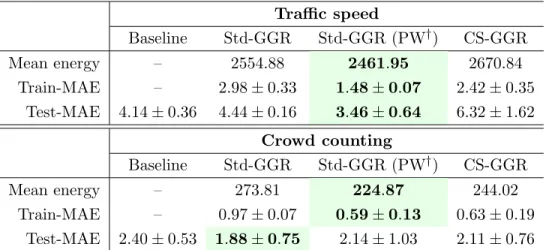
1/10). For Energy and MSE smaller values are better, for R2 larger values are better. In case of [Su et al., 2012], we fit one curve to each individual in the rat calvarium data; MSE andR2 are then averaged. . . 58 3.3 Mean energy and mean absolute errors over all CV-folds±1σon training and

testing data . . . 61 3.4 Comparison ofR2 measure and model criticism for synthetic data. *In theory, this

number should approximate 5% with enough trials, e.g., 10000. . . 80 3.5 Comparison ofR2 measure and model criticism for real data. . . 81

4.1 Comparison of the median ages estimated by functional boxplots (FB) and weighted functional boxplots (WFB) on synthetic data. ∗This measure counts the frequency with which the estimated median ages are closer to the true age for FB and WFB respectively. In 75% of the cases the median ages from these two methods are identical. . . 97 4.2 The number of data objects inside the 50% central region for functions, shapes

4.3 Comparison of the median ages estimated from the functional boxplot (FB) and the weighted functional boxplot (WFB) on the pediatric airway dataset. ∗This counts the number of the median ages that are closer to the atlas ages between functional boxplots and weighted functional boxplots; 52.94% of the median ages from these two methods are equal. . . 105 4.4 Computational cost of building an atlas based on the weighted functional boxplot. 107 4.5 P-values of two types of tests on the scores for pediatric upper airways estimated

based on weighted pointwise boxplots, functional boxplots and weighted functional boxplots. Notes: Pre represents the SGS pre-surgery group, Post represents the SGS post-surgery group, CRL represents the normal control group, and Post&CRL represents the union of the SGS post-surgery and normal control groups. . . 110 4.6 Comparison of the scores for SGS subjects using three different methods with the

clinical diagnosis based on the Myer-Cotton grading system. Notes: Weighted pointwise boxplots (WPB), functional boxplots (FB), and weighted functional box-plots (WFB). The scores are converted based on the correspondence between our scoring system and the Myer-Cotton system in Section 4.3.5. Grade I represents an obstruction within (0% - 50%]. . . 114 4.7 The confusion matrices among groups: SGS pre-surgery (Pre), SGS post-surgery

(Post), and control (CRL). Notes: P (positive), N (negative), TP (true positive), FP (false positive), FN (false negative), TN (true negative), TPR (true positive rate), FPR (false positive rate), PPV (positive predictive value), and ACC (accuracy). . 115

5.1 Distances and estimated p-values (10000 random permutations) on toy data using (1) the mean difference in Euclidean space ( ¯DE), (2) the Mahalanobis distance

( ¯DM), and (3) the Bhattacharyya distance (DB) as a test-statistic. . . 147 5.2 Distances and estimatedp-values (10000 random permutations) on synthetic shapes

using the averaged Mahalanobis distance ( ¯D_MT M) and the generalized Bhattacharyya distance (DT M_B ). The last two columns report the test results when dropping one of the initial conditions. . . 155 5.3 Distances and estimatedp-values (10000 random permutations) on corpora callosa

LIST OF FIGURES

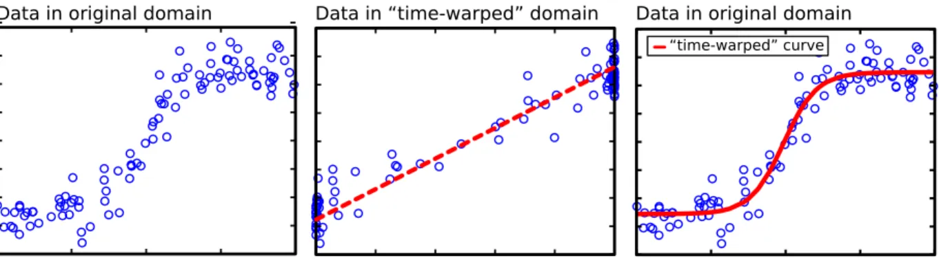
3.1 Illustration of time-warped regression inR. The dashed straight-line (middle) shows

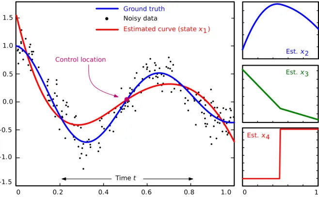
the fitting result in the warped time coordinates, and the solid curve (right) demon-strates the fitting result to the original data points (left). . . 33 3.2 Cubic-spline regression in R. The left side shows the regression result, and the

remaining plots show the other states. . . 36 3.3 CS-GGR (1 control point) vs. [Su et al., 2012] (λ1/λ2 = 10) in terms of the the

largest eigenvalue of the state-transition matrixA of Eq. (2.5) (reconstructed from the observability matrices that we obtain along each path) to the ground truth. . 53 3.4 Corpora callosa (with the subject’s age) [Fletcher, 2013]. . . 54 3.5 UCSD traffic dataset [Chan and Vasconcelos, 2005]. . . 54 3.6 Illustration of the dataset for crowd counting. Top: Example frames from the UCSD

pedestrian dataset [Chan and Vasconcelos, 2012]. Bottom: Total crowd count over all frames (left), and average people count over a 400-frame sliding window (right). 55 3.7 Comparison between Std-GGR, TW-GGR and CS-GGR (with one control point)

on the corpus callosum data [Fletcher, 2013]. The shapes are generated along the fitted curves and are colored by age (best viewed in color). . . 57 3.8 Comparison between Std-GGR, TW-GGR and CS-GGR (with one control point)

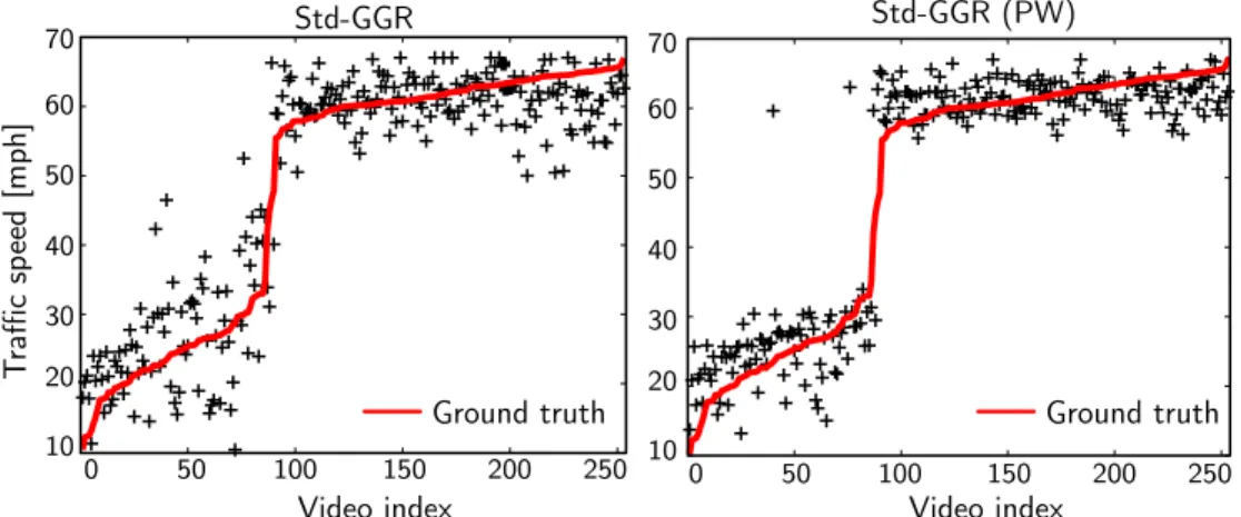
on the rat calvarium data [Bookstein, 1991]. The shapes are generated along the fitted curves and the landmarks are colored by age in days (best-viewed in color). 58 3.9 Estimated time-warp functions for TW-GGR. . . 59 3.10 Traffic speed predictions via 5-fold CV. The red solid curve shows the ground truth

(best-viewed in color). . . 62 3.11 Crowd counting results via 4-fold CV. Predictions are shown as a function of the

sliding window index. The gray envelope indicates the weighted standard deviation (±1σ) around the average crowd size in a sliding window (best-viewed in color). . 62 3.12 Bull’s eye metamorphic regression experiment. Measurement images (top row).

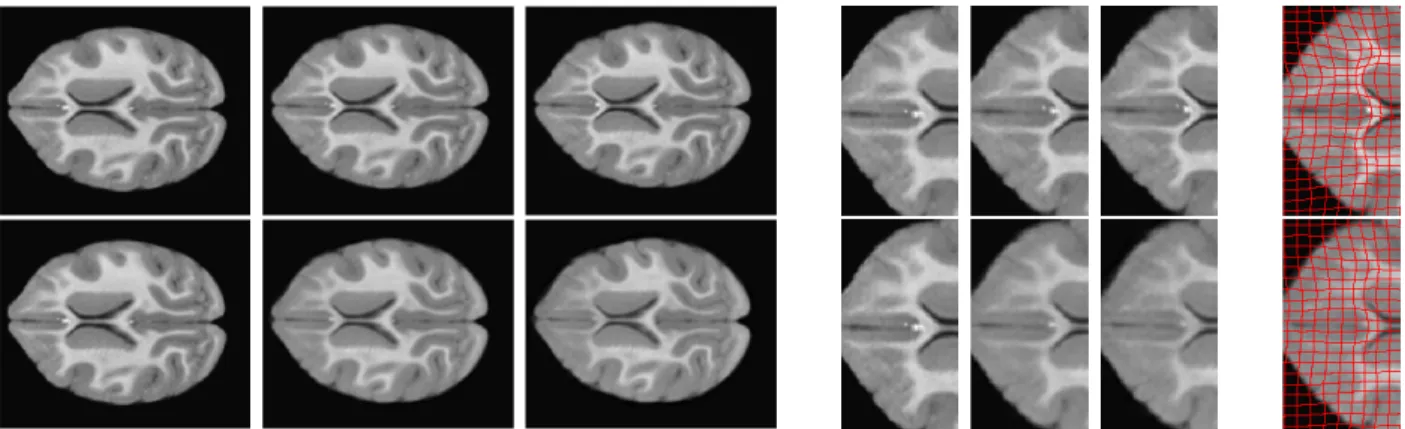
3.13 Square metamorphic regression experiment. Left: moving square with decreasing intensities and no oscillations during movement; Right: moving and oscillating square with alternating intensities. In both cases the base image is the first one. Top row: measurement images, middle row: metamorphic regression results, bottom row: momenta images (left: time-weighted average of the initial momenta, to the right: momenta of the measurement images with respect to the base image). . . . 71 3.14 Two representative image scans at 3, 6 and 12 months (left to right). . . 71 3.15 Regression results for monkey data: LDDMM (top) metamorphosis (bottom). (a)

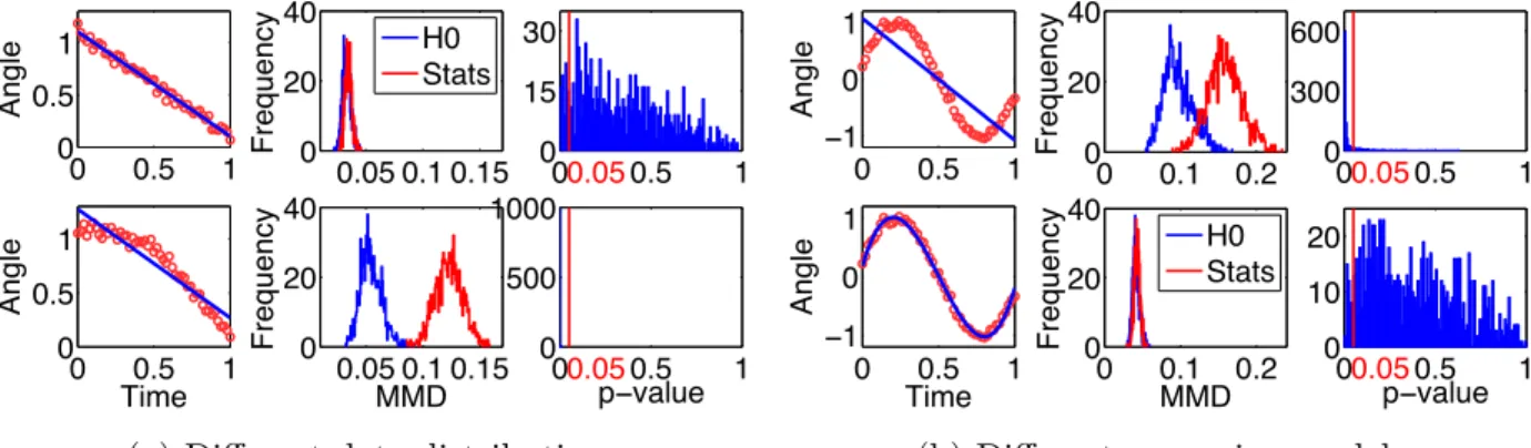
Images on geodesic at 12, 6, 3 months; (b) Zoom in for images on geodesic at 12, 6, 3 months; (c) Zoom in for images at 3 months to illustrate spatial deformation. 72 3.16 Model criticism for synthetic data on the Grassmannian. (a) Different data

distri-butions are fitted by one regression model (Std-GGR); (b) One data distribution is fitted by different regression models (top: Std-GGR, bottom: CS-GGR). . . 80 3.17 Model criticism for real data. Fromtoptobottom: the regression model corresponds

to Std-GGR, TW-GGR, and CS-GGR respectively. . . 81

4.1 (a) 20 observations generated based on Eq. (4.12) and colored by age. (b) The age histogram of the observations. . . 94 4.2 Comparisons of the atlases built by the weighted pointwise boxplot (left) and the

weighted functional boxplot (right) on the synthetic data. The atlases are adapted to the age of 85 months. The median computed by the weighted pointwise boxplot is a pointwise median, and the median computed by the weighted functional boxplots corresponds to an existing observation at 85 months. . . 95 4.3 Comparisons of atlases built by the functional boxplot (left) and the weighted

func-tional boxplot (right) on the synthetic data. The atlases are built at age 165 months and for both methods the observation at 148 months is selected as the median curve. 96 4.4 Comparison of the atlas age and the median age between the functional boxplot

(FB, the blue dashed line) and the weighted functional boxplot (WFB, the magenta dashed line). The cyan dots show the ideal case, that is, a method has a better performance if it passes through more cyan dots. The right image is a close-up view of the left one. . . 96 4.5 Comparison between the point distribution model (left) and the functional boxplot

4.6 CT scans for a control subject (left, CRL04) and a subglottic stenosis patient (right, SGS03). The zoomed-in part in the red circle shows the location of subglottic stenosis, the narrowing of the airway. . . 98 4.7 The simplified airway model for converting a 3D airway geometry to a 1D curve.

Left: the geometry segmented from a CT image, CRL04; middle: the centerline of the airway with cross sections along the centerline; right: the curve of the cross-sectional area with the depth along the centerline. . . 99 4.8 Normal curves for pediatric airway atlas construction, which are registered based

on the following five landmarks: nasal spine, choana, epiglottis tip, true vocal cord (TVC) and tracheal carina (from left to right). Zoomed-in: the sub-region from TVC to tracheal carina where the subglottis is located. . . 99 4.9 Examples of the corpus callosum shape (left) and the binary image of the

corre-sponding segmentation (right). . . 100 4.10 The functional bands (left), delimited by three corpus callosum shapes (the blue

contours), and their corresponding shape band (top right) and image band (bottom right). . . 102 4.11 Comparison between pointwise (top) and functional (bottom) boxplots on functions,

shapes and images. The black curve is the median and for the pointwise boxplots it is the pointwise median. The magenta region is the 50% confidence region. . . . 104 4.12 Age-adapted atlases for functions: pediatric airway atlases at 20 and 180

months respectively. The two airway geometries correspond to the median subjects selected by the age-matched atlases. The older atlas has a larger air-way size compared to the younger atlas, indicating the importance of building age-matched atlases. . . 105 4.13 Age-adapted atlases for shapes and images: corpus callosum atlases at 37 (top)

and 79 (bottom) years respectively. Zoomed-in: the anterior (the splenium, on the right of the atlas) and posterior (the genu, on the left of the atlas) portions of corpus callosum atlases. The atlases at different ages, especially the zoomed-in parts, clearly show the thinning of the corpus callosum with age. . . 106 4.14 The median shapes of two corpus callosum atlases at different ages and the direction

of change of the corresponding points on the boundaries. . . 106 4.15 Airway changes for two subjects, SGS03 and SGS07, pre- and post-surgery (cyan

4.16 Airway changes for SGS01 and SGS04 pre- and post-surgery. For both subjects, before surgery there is a tracheostomy tube in the airway. After surgery the sub-glottic stenosis is resolved. Compared with the age-matched atlas almost all of the corresponding curve is within the maximal non-outlying envelope, indicating a successful surgery. . . 108 4.17 The scores for all subjects, including three groups, SGS pre-surgery, SGS

post-surgery and control subjects, based on the atlases built by weighted pointwise box-plots, functional boxbox-plots, and weighted functional boxplots (from left to right). The curves in different colors represent the kernel density estimations for different groups. Note: the y-axis in the plots is a random height to visualize the scores clearly.109 4.18 Two control subjects, represented by colored dashed curves and their age-matched

atlases. The curves obtain negative scores when using the functional boxplot and non-negative scores when using the weighted functional boxplot. . . 113 4.19 Quantitative comparison of the scores for four SGS subjects before and after surgery

using functional boxplots and weighted functional boxplots for atlas-building.. . . 115 4.20 Three outliers in Fig. 4.17 for both functional boxplots and weighted functional

boxplots. (a) SGS09 is post-surgery while having a low score more consistent with a pre-surgery subject; (b) SGS13 is pre-surgery while mixed into the post-surgery group; (c) SGS08 is post-surgery appearing as a normal control subject consistent with near normal post-operative airway. . . 117

5.1 Comparison between two types of models for capturing shape variations. The three shapes in PDM (a) correspond to the mean and varying shapes along the first mode at±3 standard deviations. In DOM (b), the red shape is the median of the shape population and the grey area is the region covered by 50% of the shapes at the top ranking list of the populations, similar to the inter-quartile range (IQR) for scalar values visualized as part of a box-plot. . . 120 5.2 Overview of the depth-ordering-based shape analysis. Based on the depth and the

ordering of a shape population, statistical tests are defined to globally separate control and disease groups using global analysis with a scalar value (depth) for each shape. Statistical difference for global analysis results can be established through permutation testing. Equivalently, local shape differences can be detected using local analysis with a corresponding local permutation test, resulting in p-values on the surface of a shape to establish local shape differences between populations. The directionality of the shape differences (inflation versus deflation) can also be determined.. . . 121 5.3 Illustration of the computational complexity of band-depth calculation for all

5.4 Illustration of global shape analysis. A group of control subjects is chosen as a training set, and the band-depth of each test shape from control or disease groups, is computed with respect to the training set. The boxplots on the right show that in general the control group would have larger depths than the disease group if control subjects are selected as the reference/training population. . . 127 5.5 Global shape analysis on synthetic data using band-depth computed with (a) and

without (b) a training population. The training population allows detection of global shape differences. . . 128 5.6 Illustration of the median andα-central region. The median function / shape (red)

is the most central one of a population, and the α-central region (grey) is the band delimited by theα proportion of the deepest functions/shapes. For example, the grey region is the 0.6-central region because it is built by three out of five functions/shapes. . . 130 5.7 Illustration of local shape analysis. Reference shape population (a) (blue contours)

defines a centrality map (b) (light yellow to dark red corresponds to the most to the least central region of the reference population), which provides a local measure (c) (α-values) of how deeply a test shape (the non-ellipse shape) is buried with respect to the reference population. The dilated region is colored by the darkest red with

α-values greater than 1. . . 132 5.8 Illustration of directionality for a template shape (the ellipse with a bump and an

indented region) with respect to the median shape (the ellipse at the zero level-set) of a reference population.. . . 134 5.9 Ground-truth of a sample shape (two views from the lateral and medial sides).

Colormap on the shape indicates the location and magnitude of the artificial de-formations compared to the undeformed shape. Red color corresponds to a large deformation distance.. . . 135 5.10 Local shape analysis on synthetic striatum shown from two views, the medial (top)

and the lateral (bottom) views, with the median of NC-Test as the template and the disease test group as the reference. (a) The α-values on the template. (b) The corresponding raw p-values with 10000 permutations and FDR corrected p -values. (c) The directionality of shape differences on the template with respect to the median of the reference group. . . 136 5.11 Local shape analysis on synthetic striatum shown from two views, the medial (top)

5.12 The directionality of shape differences on the median test shapes with respect to the median shape of the NC-Train group shown from two views, lateral (left) and medial (right) sides. . . 138 5.13 Global analysis on both left and right hippocampi. The disease group indicates

subjects with first-episode schizophrenia.. . . 140 5.14 Local analysis on the disease median of both left and right hippocampi with respect

to the normal control test group. . . 141 5.15 A toy example in Euclidean space. Top: (a) Cross-sectional data of two groups,

illustrated as red circles and blue squares; (b) the same data with longitudinal information where points on the same line are observations from one subject; (c) the trajectory space, represented by a slope and an intercept. Every point in this space corresponds to a straight line in (b). Bottom: (d) Trajectories generated by points along the 1st principal component (PC) of standard PCA in trajectory space with{0,±1,±2}standard deviations (SD); (e) trajectories generated along the 2nd PC (best-viewed in color). . . 145 5.16 Synthetic shapes: (a) Basic shapes used to generate the population on the right;

(b) and (c) show the two groups of trajectories (best-viewed in color). . . 154 5.17 Visualization of the variances (left) and principal directions (right) of trajectory

distributions for the synthetic data (best-viewed in color). . . 154 5.18 Visualization of the variances (left) and principal directions (right) of trajectory

CHAPTER 1 : INTRODUCTION

1.1 Motivation

Spatiotemporal data analysis frequently arises in medical research and computer vision problems. Examples include MRI (magnetic resonance imaging) time-series collected to explore brain development [Evans et al., 2006], corpus callosum shapes at varying ages ob-tained to analyze the degeneration process of a single brain structure [Fletcher, 2013], and traffic video clips acquired by a surveillance system monitoring highway traffic to classify con-gestion in traffic sequences [Chan and Vasconcelos, 2005]. Analysis of this spatiotemporal data, e.g., image time-series, shape sequences, and videos, is an important topic in the field of computer vision and medical image analysis. In this dissertation, this topic will be explored from three aspects: 1) capturing time-varying changes within a subject or a population, e.g., studying brain development or a disease process; 2) estimating a spatiotemporal atlas while retaining population variation information, e.g., a pediatric airway atlas with a confidence region; and 3) identifying shape differences between populations, e.g., to differentiate normal control subjects from subjects with disease.

diffeomorphisms [Banyaga, 1997], Kendall shape space [Kendall, 1984], or the Grassmannian [Edelman et al., 1998]. Although a manifold resembles Euclidean space in the neighborhood of each point, globally it may not. As a result, methods developed in Euclidean space cannot be directly applied to the spatiotemporal data explored in this dissertation.

1.1.1 Estimation of Time-Varying Changes

Time-varying changes occur in spatiotemporal data, which is collected to study, for ex-ample, aging [Scahill et al., 2003], disease progression [Kogure et al., 2000], and brain devel-opment [Evans et al., 2006]. To summarize these changes within a subject or a population, regression analysis is popular, because it is a powerful tool to model the relationship between data objects [Marron and Alonso, 2014] and their associated descriptive variables, e.g., age. Recently, regression models [Niethammer et al., 2011, Fletcher, 2013] have been proposed to estimate changes in shape or image time-series by generalizing linear regression in Eu-clidean space to Riemannian manifolds [Lee, 2012] and the manifold of diffeomorphisms respectively. An interesting problem is to develop auniformframework of parametric regres-sion, which arises when changes in different types of spatiotemporal data are to be captured using the equivalent of linear or higher-order fitting curves in non-Euclidean spaces. For in-stance, the collected data could be shapes or videos. While a regression model equivalent to linear curve fitting [Niethammer et al., 2011, Fletcher, 2013] is relatively simple, sometimes it may be too restrictive for data exhibiting more complex changes. In such cases, higher-order polynomial or spline fitting curves [Hinkle et al., 2014, Singh and Niethammer, 2014] can be attractive, but their formulations are typically complicated.

check models’ underlying assumptions. To achieve this, I first represent data objects, e.g., shapes or videos, as elements on the Grassmannian, using singular value decomposition (SVD) [Begelfor and Werman, 2006, Sepiashvili et al., 2003] and a dynamic texture model [Doretto et al., 2003] respectively. Then optimal control approaches are applied to develop regression models of increasing order on the Grassmannian. In existing work, two groups of solutions are presented to solve parametric regression problems in the spaces of shapes or images: 1) geodesic shooting based strategies that address the problem using adjoint methods from an optimal-control point of view [Niethammer et al., 2011, Hong et al., 2012a, Singh et al., 2013b], and 2) approaches that compute the required gradients using Jacobi fields for optimization [Rentmeesters, 2011, Fletcher, 2013]. Unlike Jacobi field approaches, solutions using optimal control methods do not require the computation of curvatures explic-itly and can be easily extended to higher-order models, e.g., polynomials [Hinkle et al., 2014] or splines [Singh and Niethammer, 2014]. Hence, the strategy based on geodesic shooting is adopted to develop extensible solutions on the Grassmannian, i.e., extending the basic model to time-warped and cubic-spline variants. Overall, a uniform framework for parametric re-gression on the Grassmannianis proposed to solve fitting problems with models of increasing order for different types of spatiotemporal data that can be represented as elements on the Grassmann manifold.

after image registration exist [Rohlfing et al., 2009], this dissertation develops a regression model that captures spatial deformations and intensity changes simultaneously. This can be achieved by using a metamorphic regression formulation, which combines the dynamical system formulation for geodesic regression on images [Niethammer et al., 2011] with image metamorphosis [Holm et al., 2009, Miller and Younes, 2001] for the large displacement dif-feomorphic metric mapping (LDDMM) registration model [Beg et al., 2005]. The resulting proposed model is called metamorphic geodesic regression on image time-series.

1.1.2 Estimation of A Spatiotemporal Statistical Atlas

Atlas-building from population data has become an important task in medical imag-ing to provide templates for data analysis. Numerous methods for atlas-building exist, ranging from methods designed for cross-sectional, longitudinal, and random design data [Joshi et al., 2004, Fletcher et al., 2009, Hart et al., 2010]. These approaches typically esti-mate a representative data object (such as a shape, a surface, or an image) for a population, e.g., a mean [Joshi et al., 2004] (or a time-adjusted population mean [Hart et al., 2010]) or a median [Fletcher et al., 2009] with respect to spatial deformations and appearance.

[Aljabar et al., 2009] suggest a multi-atlas approach to estimate multiple representers of the population. In another study, [Gerber et al., 2010] propose to learn a low-dimensional representation driven entirely by the population of images.

Another strategy to retain population variation is to represent additional aspects of the full data distribution, such as percentiles, the minimum and maximum, variance, confidence regions and outliers as captured by a boxplot for scalar-valued data. The functional box-plot [Sun and Genton, 2011] is an effective tool to represent such statistics for functions. Generalizing the notion of functional boxplots to summarize variabilities within a popula-tion of entities such as shapes and images provides a simple and generic method to augment a single representer with additional population information. Besides, as subject data typ-ically has associated individual characteristics (e.g., age, weight, and gender), a method is expected to be able to compute the statistical information parameterized by these charac-teristics. For example, given a subject at a particular age the goal is to compute subject age-specific confidence regions to assess similarity with respect to the full data population.

Hence, a weighted variant of the functional boxplot is developed in this dissertation to enable the use of kernel regression for estimating a regressed curve with local distributional information. If each data object on the regressed curve, with its additional statistical infor-mation, is treated as a statistical atlas, this non-parametric regression model can be regarded as a model to build a spatiotemporal statistical atlas, which is referred to asstatistical atlas construction via weighted functional boxplot.

1.1.3 Statistics of Group Differences

data. For example, in the studies of Alzheimer’s disease (AD), which accounts for 60% to 70% of cases of dementia [Burns and Iliffe, 2009], researchers are interested in whether brain shapes of normal control subjects are significantly different from those of subjects with disease and where shape differences are located. To answer these questions, analysis approaches have been proposed to assess object properties and are used to characterize shape variations across subjects and between subject populations [Nitzken et al., 2014]. Most of these shape analysis methods are based on the classical point distribution model (PDM) [Cootes et al., 2004], and the PDM requires some form of point-to-point correspondences between shapes to allow pre-cise local shape analysis. However, establishing these correspondences is highly non-trivial and arguably one of the main sources of inaccuracy. Because any misregistration may cre-ate artifacts in the final shape analysis results. Recently, shape characterizations have been explored based on concepts of order statistics [Whitaker et al., 2013, Hong et al., 2014a]. These methods utilize depth-ordering of shapes, for example, to generalize the median and the inter-quartile range (IQR) to shapes, effectively obtaining the equivalent of a boxplot for shapes. Using shape-descriptions based on depth-ordering makes it possible to perform shape analysis with very limited (e.g., rigid or affine) spatial alignment of shapes. Further-more, it can avoid having strong distributional assumptions of the data population, e.g., an assumption of Gaussian distribution. Therefore, to address the problem of differenti-ating subject populations, a statistical testing method based on depth-ordering on shapes is proposed to detect potential global and local shape differences, which is referred to as depth-ordering-based shape analysis.

1.2 Thesis Statement

Thesis: Advanced regression models or a time-varying statistical atlas can efficiently cap-ture individual or population changes in spatiotemporal image and shape data. Statistical

differences between shape populations can be detected using depth-ordering and statistics on

shape trajectories.

The contributions of this dissertation are:

1. A uniform framework ofparametric regression on the Grassmannianhas been proposed to capture both linear and non-linear changes. It handles regression formulations with different orders, including standard geodesic regression, time-warped geodesic regression, and cubic spline regression.

2. A model of metamorphic geodesic regressionhas been proposed to simultaneously cap-ture spatial deformations and intensity changes in image time-series. It is efficiently solved using a simple, approximate algorithm via pairwise shooting metamorphosis.

3. Amodel criticismfor regression models on manifolds, e.g., the Grassmannian manifold, has been proposed to check if model assumptions hold, using kernel two sample tests.

4. A model for building a spatiotemporal statistical atlas has been proposed based on kernel regression and a weighted variant of the functional boxplot. It can construct a series of time-varying atlases, augmented by the local distribution of spatiotemporal data, e.g., confidence bounds or outliers. It has been applied to time-varying functions, shapes, and images.

making strong distributional assumptions. It has been applied to analyze and compare populations, e.g., normal controls and subjects with disease.

6. A model of hypothesis testing for longitudinal data has been proposed by leveraging shape trajectories and their second-order statistics, i.e., variances of trajectory distri-butions, to identify group differences of shapes.

1.3 Overview of Chapters

The remainder of this dissertation is organized in the following chapters:

Chapter 2 provides an overview of the required background in this dissertation, including the necessary background for image and shape analysis and the mathematical background for some manifolds discussed in this dissertation.

Chapter 3 presents parametric regression models on two types of smooth manifolds, i.e., the Grassmann manifold and the manifold of diffeomorphisms.

Chapter 4 presents the model for building a spatiotemporal statistical atlas.

Chapter 5 presents two hypothesis testing approaches to identify shape differences be-tween populations for cross-sectional and longitudinal data respectively.

CHAPTER 2 : BACKGROUD

This chapter presents some necessary background material required in this dissertation. In particular, the mathematical background is briefly reviewed in Section 2.1, including some concepts in smooth manifolds and the Riemannian structure of the Grassmann manifold, as well as how to represent data objects as elements on the Grassmannian. The background for image and shape analysis is presented in Section 2.2. It starts with an overview of fundamental problems in image analysis, e.g., image registration and shape representations. The review of regression models, atlas construction, and statistical hypothesis testing aims to help promote a better understanding of the following chapters of this dissertation.

2.1 Mathematical Background

2.1.1 Smooth Manifolds

In general, smooth manifolds [Lee, 2012] are spaces that locally look like Euclidean space

Rn, but globally they may not, e.g., spheres. To be a smooth manifold, a space should first be atopological manifold, the most basic type of manifold. In particular, a topological space M is a topological manifold of dimension n or a topological n-manifold, if it has the following properties:

• M is a Hausdorff space: for every pair of points p, q ∈ M, there are disjoint open subsets U, V ⊂M such that p∈U and q ∈V.

• M is locally Euclidean of dimension n: every point of M has a neighborhood that is homeomorphic to an open subset of _Rn_.

Apart from the topology, a smooth manifold also needs some extra structure, which allows to define calculus for computation of smooth functions on the manifold. For two open subsets U and V from Euclidean spaces _Rn _and

Rm respectively, a function/map F : U → V is smooth (orC∞, orinfinitely differentiable) if each of its component functions has continuous partial derivatives of all orders. Furthermore, if F is bijective and has a smooth inverse map, it is called a diffeomorphism. In particular, a diffeomorphism is a homeomorphism. Given two neighborhoods U, V in a manifold M, two homeomorphisms x : U → _Rn _and y : V → _Rn _{are C}∞_{-related if the composite maps x◦y}−1 _{: y(U ∩V) → x(U ∩V) and} y◦x−1 :x(U ∩V)→y(U ∩V) areC∞. Here, the pair (x, U) is called a chart orcoordinate system. A collection of charts whose domains cover M is called an atlas for M. If any two charts in an atlas are smoothly compatible with each other, this atlas is called asmooth atlas. And a smooth structure on a manifold M is a maximal smooth atlas on M. The manifold M along with such an atlas is defined as a smooth manifold [Lee, 2012].

Tangent spaces. LetM be a smooth manifold, and let pbe a point ofM, associated with smooth real-valued functions f : M → _R. The set of all derivatives of C∞(M) at p is a vector space called the tangent space to M at p, which is denoted by TpM. An element of TpM is called a tangent vector at p[Lee, 2012].

on its tangent space TpM [Do Carmo, 1992].

Geodesics. Using the Riemannian metric, we can compute the length of a curve on a smooth manifold. In Euclidean space, the length of a straight line connecting two points is the shortest path between them. Accordingly, the shortest smooth curve segment between two points on a manifold is a geodesic.

2.1.2 Riemannian Structure of the Grassmannian

The Grassmannian is an example of a smooth manifold with a Riemannian structure. The Grassmann manifold G(p, n) is defined as the set of p-dimensional linear subspaces of

Rn, typically represented by an orthonormal matrix Y ∈ Rn×p, such that Y = span(Y) for Y ∈ G(p, n). It can equivalently be defined as a quotient space within the special orthogonal group SO(n) as G(p, n) :=SO(n)/(SO(n−p)× SO(p)). The canonical metric gY :TYG(p, n)× TYG(p, n)→R onG(p, n) is given by

gY(∆Y,∆Y) = tr ∆>Y∆Y = tr C>(In−YY>)C , (2.1)

where In denotes the n×n identity matrix, TYG(p, n) is the tangent space atY, ∆Y is the

tangent vector in TYG(p, n), and C ∈ Rn×p is arbitrary. For the Grassmann manifold this essentially computes the distance between subspaces [Edelman et al., 1998]. Typically, the principal angles between two subspaces are used to measure their distance. This measure can be understood as an arc length distance. Under this choice of metric, the arc-length of the geodesic connecting two subspaces Y,Z ∈ G(p, n) is related to the canonical angles

φ = {φ1, . . . φp} ∈ [0, π/2] between Y and Z as d2g(Y,Z) = ||φ||22. Next, the notation is slightly changed and d2

the (squared) geodesic distance can be computed via SVD, i.e., U(cosΣ)V> = Y>Z as d2

g(Y,Z) =||diagΣ||2, where Σis diagonal with principal angles φi, or UΣ0V> =Y>Z as d2_g(Y,Z) = ||cos−1(diagΣ0)||2 _{(cf. [Begelfor and Werman, 2006]). There are other} defini-tions of the distance between two subspaces, e.g., the chordal 2-norm and Frobenious-norm distances. They are defined by embedding the Grassmann manifold in the vector space_Rn×p [Edelman et al., 1998]. Since the arc length distance is derived from the intrinsic geometry of the Grassmann manifold, it is chosen as the geodesic distance of the Grassmannian in this dissertation.

Now, consider a curve γ : [0,1]→ G(p, n), r7→ γ(r) such that γ(0) = Y0 and γ(1) = Y1, with Y0 represented by Y0 and Y1 represented by Y1. The geodesic equation for such a curve, given that ˙Y=d_{/drY(r)= (}. _I

n−YY>)C, on G(p, n) is given by

¨

Y(r) +Y(r)[ ˙Y(r)>Y˙(r)] = 0 , (2.2)

which also defines the Riemannian exponential map on the Grassmannian as an ODE (ordi-nary differential equation) for convenient numerical computations. This can be derived by solving an optimization problem from the calculus of variations. It minimizes the distance between two points on the Grassmann manifold, i.e., Eq.(2.1), under the constraints of the above definition for a tangent vector and keeping to be an orthonormal matrix along the geodesic, i.e., Y>Y =I. Integrating Eq. (2.2), starting with initial conditions we can shoot the geodesic forward in time.

Exponential map. The exponential map (Exp-map) maps a point Y = span(Y) with a direction D in the tangent spaceTYG(p, n) to a pointZ = span(Z) on the manifold G(p, n),

i.e.,

Exp_Y(tD) =Z, t ∈[0,1]

along the geodesic that connects Y and Z. By letting D = UΣV> denote the compact SVD ofD, the Exp-map onG(p, n), in terms of representers Y and Z, can be written as (cf. [Begelfor and Werman, 2006])

Z=YVcos(tΣ)V>+Usin(tΣ)V> . (2.3)

Here, becauseΣis a diagonal matrix,cos(tΣ) and sin(tΣ) are also diagonal matrices. They can be computed by simply taking the sines or cosines on the matrices’ diagonal components. The proof of this formulation can be found in [Edelman et al., 1998].

Inverse exponential map. The inverse exponential map (Log-map) computes the mapping from a neighborhood U ⊂ G(p, n) of Y to TYG(p, n). In terms of representers Y,Z for the

subspaces Y = span(Y),Z = span(Z), the Log-map can be written as H = Log_Y(Z). In other words, H is the direction matrix which allows starting at Y and walking along the geodesic in the direction of H to reach Z in unit time (t = 1), i.e., Z = Exp_Y(H). Let H=UΣV>. Multiplying Eq. (2.3) with Y> on the left-hand side (andt = 1) results in

Y>Z =Y>Y

| {z } =Ip

Vcos(Σ)V>+Y>U

| {z } =0

sin(Σ)V>=Vcos(Σ)V> .

YY>Z .Thus

Usin(Σ)V>(Vcos(Σ)V>)−1 = (Z−YY>Z)(Y>Z)−1,

which – upon noting that (1) (Vcos(Σ)V>)−1 =Vcos(Σ)−1V>and (2)V>V =Ip– reduces to

Utan(Σ)V> = (Z−YY>Z)(Y>Z)−1 .

This yieldsH via the SVD of (Z−YY>Z)(Y>Z)−1 _{(or Z(Y}>_Z)−1_{−Y) as}

H= Log_Y(Z) =Uarctan(Σ)V> .

Parallel transport. Given two subspaces X,Y, represented via X,Y and a direction matrix H ∈ TXG(p, n) such that Y = ExpX(H), the objective is to transport an arbitrary

tangent vector∆atTXG(p, n) toTYG(p, n) along the geodesic connectingX andY. Letting

H=UΣV>, parallel transport (denoted byτ) can be computed via [Edelman et al., 1998]

τ∆(t) =−YVsin(tΣ)U>∆+Ucos(tΣ)U>+ (In−UU>)∆, t∈[0,1] . (2.4)

2.1.3 Representation on the Grassmannian

This dissertation describes two types of data that can be represented on G(p, n): linear dynamical systems (LDS) and shapes (see shape representation in Section 2.2.2).

with yi ∈_Rn_{, the standard dynamic texture model with p states has the form}

xk+1= Axk+wk, wk∼ N(0,W),

yk= Cxk+vk, vk ∼ N(0,R) , (2.5)

withxk∈Rp,A∈Rp×p, andC∈Rn×p. When relying on the prevalent system identification of [Doretto et al., 2003], the matrix C is, by design, of (full) rank p (i.e., the number of states) and by construction an observable system [Kalman, 1959] is obtained, where a full rank observability matrix O ∈ _Rnp×p _{is defined as O = [C (CA) (CA}2_{) · · · (CA}p−1_)]>_.

This system identification using the dynamic texture model is not unique. Because systems (A,C) and (TAT−1,CT−1) with T∈ GL(p) have the same transfer function, i.e., with the same input they have the same output. Hence, the realization subspace spanned by O is a point on the Grassmannian and the observability matrix is a representer of this subspace. An LDS model is identified for a video by its np×p orthonormalized observability matrix.

To support a non-uniform weighting of samples during system identification, atemporally localized variant of [Doretto et al., 2003] is proposed in this dissertation. This is beneficial in a situation where a considerable number of frames are needed for stable system identification, yet not all samples should contribute equally to the LDS parameter estimates. Specifically, given the measurement matrixM = [y1,· · · ,yτ] and a set of weightsw= [w1,· · · , wτ] such that P

iwi =τ, a weighted SVD of M is computed as

UΣV>=M diag(√w) . (2.6)

been determined, A can be computed as A = Xτ₂W12(Xτ−1 1 W

1

2)†, where † denotes the pseudoinverse, Xτ

2 = [x2,· · ·,xτ],X1τ−1 = [x1,· · · ,xτ−1] and W 1

2 is a diagonal matrix with W

1 2

ii = [ 1

2(wi+wi+1)] 1/2_.

Shapes. Let a shape be represented by a collection of m points. A shape matrix is con-structed from itsmpoints asL = [(x1, y1, ...); (x2, y2, ...);. . .; (xm, ym, ...)]. By applying SVD on this matrix, i.e.,L =UΣV>, an affine-invariant shape representation is obtained by us-ing the left-sus-ingular vectors U [Begelfor and Werman, 2006, Sepiashvili et al., 2003]. This establishes a mapping from the shape matrix to a point on the Grassmannian (withUas the representative). Such a representation has been used for facial aging regression, for instance [Turaga et al., 2010].

2.2 Image and Shape Analysis Background

2.2.1 Image Registration

Image registration is one of the fundamental research topics in image analysis. It is the process of placing different images into geometrical and/or anatomical agreement. Typically, images of the same scene are taken at different times, from different viewpoints, and/or different modalities. The regression problem presented in Chapter 3 can be reduced to an image registration problem if there are only two images. Hence, some necessary knowledge about image registration is presented here before the discussion of regression models. A detailed review of image registration in computer vision and medical image analysis can be found in [Zitova and Flusser, 2003] and [Oliveira and Tavares, 2014], respectively.

image, that is, the cost function. In addition, the cost function usually includes another term, a regularization term, to enforce smoothness of the geometric transformation. In general, there are three components needed for formulating an image registration problem: the geometric transformation, the similarity measure, and the regularization term discussed in the following.

Usually, the geometric transformations can be divided into two categories: rigid and non-rigid transformations. Rigid transformations are the simplest cases, typically estimating the parameters of translation and rotation. Non-rigid transformations include the similarity transform, affine, projective, and curved (elastic or fluid) transformations. In this disserta-tion, the image regression is built upon the large deformation diffeomorphic metric mapping (LDDMM) model [Beg et al., 2005], which is a representative of the fluid-based registration. The similarity measures are mostly divided into two types of methods: intensity and feature-based approaches. The commonly-used measures in the category of intensity-based similarity include the sum of squared differences (SSD) and the mutual information (MI). The underlying assumption of SSD is that the structures of interest in both images should have identical intensities. Hence, a lower SSD value indicates a better registration result. In contrast, MI captures how well one image explains the other. Hence, for this measurement a higher MI value indicates a better registration result. On the other hand, in the category of the feature-based similarity measures, the similarity measures focus on computing the differences of structures extracted from images. The feature could be smaller image patches or volumes compared via their intensity differences or corresponding points compared via their Euclidean distances.

A commonly-used one is related to the second-order derivations of the transformation or the Jacobian of the transformation. In the following the LDDMM will be treated as a concrete example to discuss the non-rigid image registration, in particular the fluid flow registration. Fluid flow registration and LDDMM [Beg et al., 2005]. As discussed before, the objective of image registration is to deform a source image I0 (or the moving image) to match a target image I1 (or the static/template image), as accurate as possible. In fluid flow registration, the deformation (i.e., the transformation used in the previous part) is parametrized through a spatiotemporal velocity field v. It “flows” the image I0 to another image I1 under a transport equation

It+∇I>v = 0, I(0) = I0 . (2.7)

To ensure the smoothness of the velocity filed, it is meaningful to combine the intensity-based similarity term with a regularity term, resulting in a cost function of the form

E(I, v) = 1 2

Z 1

0 kvk2

L dt

| {z }

Regularity

+ 1

σ2 kI(1)−I1k 2

| {z }

Similarity

, (2.8)

where kvk2

L = hLv, Lvi and L is a differential operator to encourage smoothness of the velocity field. Typically, L = −α∇2 _{+γ, and α and γ are constants. This cost function} should be minimized with respect to the dynamic constraint in Eq. (2.7).

To solve this optimization problem, the dynamic constraint is added as an equality con-straint through a Lagrangian multiplier λ, which has the same size with the image I, i.e.,

E(I, v, λ) = 1 2

Z 1

0 kvk2

L dt+ 1

σ2kI(1)−I1k

2_{+hλ, I}

then optimality conditions can be obtained through variational calculus, resulting in

         

        

It+∇I>v = 0, I(0) =I0,

−λt−div(λv) = 0, λ(1) = _σ22(I1−I(1)),

v+ (L†L)−1_{λ∇I = 0 .}

(2.10)

Here, L† denotes the adjoint of L. There are two commonly-used optimization methods for LDDMM to obtain a numerical solution, the relaxation optimization and the shooting optimization.

In relaxation optimization the velocity field at every time point is updated in each iter-ation. It proceeds as follows

• Given an estimation for the velocity field v, flow the intensity I forward according to

the first equation in Eqs. (2.10).

• Compute the solution for the adjointλ backward in time using the second equation in

Eqs. (2.10).

• Compute the gradient for the velocity v at every point in time using the equation ∇vE =v+ (L†L)−1(λ∇I).

• Update the estimate for the velocity v using a gradient descent step.

• Repeat the previous steps until convergence.

and v(0) are of the interest. Actually, given λ(0) (the so-called initial momentum) we can compute the initial velocity v(0) using the image I0 and the third equation in Eqs. (2.10). This can save memory resources during the computation. In particular, the shooting opti-mization is derived according to the fact that the energy is conserved along the geodesic. Then, the regularity term can be rewritten using initial conditions only, i.e., the initial image and the initial velocity. From now on, the adjoint λ will be replaced with the notation p to represent the momentum, because new Lagrangian multipliers will be introduced in the shooting formulation. Since the velocity field v =−(L†L)−1_{p∇I, we can derive}

kvk2

L =hLv, Lvi=hv, L

†

Lvi=h(L†L)−1p∇I, p∇Ii . (2.11)

WithK = (L†L)−1_{, we obtain the new cost function in form of}

E(I(0), p(0)) = 1

2hp(0)∇I(0), K∗p(0)∇I(0)i+ 1

σ2kI(1)−I1k

2 _{. (2.12)}

This cost function is minimized under the constraints of the relaxation optimality conditions:

         

        

It+∇I>v = 0, I(0) =I0, pt+div(pv) = 0,

v+K∗p∇I = 0,

(2.13)

then we compute the adjoint model through variational calculus. As a result, we obtain

         

        

λI

t +div(λIv+pK∗λv) = 0, λI(1) = σ22(I1−I(1)), λp_t + (∇λp₎>_{v− ∇I}>_K∗λv _{= 0, λ}p_{(1) = 0,}

λv_+λI_{∇I− ∇λ}p_{p = 0 .}

(2.14)

According to Eq (2.14), we can shoot backward to update the initial momentum using

∇p(t0)E =−λ

p_{(0) +∇I}>

0 K∗(p(0)∇I(0)), (2.15)

which is the gradient obtained through the variational calculus for the Lagrangian function. Note that, the initial image is not required to be updated, because it is fixed. Besides, solving transport equations can be non-trivial for non-smooth functions. In practice, instead of solving It+∇I>v = 0 we solve

Φt+DΦv = 0, Φ(0) =id, (2.16)

where Φ is the deformation map for the coordinate mapping and id is the identity map. Then, the intensity I at each time point can be estimated by I(t) = I0 ◦Φ(t). Similarly, given a backward solution to

−Φb_t −DΦbv = 0, Φb(1) =id, (2.17)

smooth maps, which are much easier to propagate numerically.

2.2.2 Shape Representation

In [Dryden and Mardia, 1998], shape is defined as all the geometrical information that remains when location, scale, and rotational effects are filtered out from an object. This

defi-nition has been generalized to mean “a shape is the spatial information after an equivalence group of geometric transformations are filtered out, for example, the group of similarity transformations”. There are different shape representations. In this dissertation the shape is represented in two ways: 1) point-based representation, i.e., describing a shape with a finite number of points on its boundary; and 2) binary representation with 1 indicating the inside of a shape and 0 outside. Besides, other shape representations exist, e.g., the surface-based representations [Dale et al., 1999], and the medial representations (e.g., m-reps [Pizer et al., 2003]).

In particular, a point-based shape can be represented as an element on the Grassman-nian, as discussed in Section 2.1.3. This representation is designed for shapes after remov-ing the effects of translation, rotation, and non-uniform scalremov-ing. In some other scenarios where uniform scaling is considered instead of non-uniform scaling, the Kendall shape space [Kendall, 1984] is one possible choice for the shape representation. For example, in Chapter 5, geodesic regression on Kendall shape space from [Fletcher, 2013] will be used to summa-rize a shape trajectory for each subject with longitudinal shape data. Therefore, some basic concepts in the Kendall shape space is presented here, including the required computation of Exponential/Log maps for geodesic regression. For more detailed explanations about the Kendall shape space, please refer to [Kendall, 1984] and [Fletcher, 2013].

z ∈_Ck_{. After removing translation, rotation and scaling, a shape can be treated as a point} in the complex projective space _CPk−2. Given a centered shape x and the initial velocity v, which is a tangent vector at x, such thathx, vi= 0, the exponential map is given by

Exp_x(v) = cosθ·x+kxksinθ

θ ·v, θ=kvk . (2.18)

The Log-map computes the initial velocity between two shapes x and y and is given by

Log_x(y) = θ·(y−πx(y)) ky−πx(y)k

, θ= arccos |hx, yi|

kxkkyk, (2.19)

where πx(y) =x· hx, yi/kxk2 denotes the projection of the vector y ontox.

2.2.3 Regression Models

Regression models presented in Chapter 3 are representatives of theparametric category, in particular, on smooth manifolds. Although differential geometric concepts, e.g., geodesics and intrinsic higher-order curves, have been well-studied in the literature [Noakes et al., 1989, Camarinha et al., 1995, Crouch and Leite, 1995, Machado et al., 2010], their use for para-metric regression, i.e., finding parametric relationships between the manifold-valued vari-able and an independent scalar-valued varivari-able, has only recently gained interest. A variety of methods extending concepts of regression in Euclidean space to nonflat manifolds have been proposed. [Rentmeesters, 2011, Fletcher, 2013] and [Hinkle et al., 2014] address the problem of geodesic fitting on Riemannian manifolds. They primarily focus on symmetric spaces, to which the Grassmann manifold belongs. [Batzies et al., 2015] study a theoretical characterization of fitting geodesics on the Grassmannian. And [Niethammer et al., 2011] generalize linear regression to the manifold of diffeomorphisms to model image time-series data, followed by work extending this concept [Hong et al., 2012a, Singh et al., 2013b] and enabling the use of higher-order models [Singh and Niethammer, 2014].

Regression on the Grassmann manifold. In the context of computer-vision problems, [Lui, 2012] recently adapted the known Euclidean least-squares solution to the Grassman-nian. While this strategy works remarkably well for the presented gesture recognition tasks, the formulation does not guarantee the minimization of the sum-of-squared geodesic distances within the manifold, which would be the natural extension of least-squares to Riemannian manifolds. Hence, the geometric and variational interpretation of [Lui, 2012] remains un-clear. In contrast, this dissertation addresses the problem from the aforementioned energy-minimization point of view which guarantees, by design, consistency with the geometry of the manifold.

To the best of my knowledge, the most related work to the regression models in this dissertation is [Rentmeesters, 2011, Fletcher, 2013] and [Batzies et al., 2015] in the context of fittinggeodesics, as well as [Machado et al., 2010] (and to some extent [Hinkle et al., 2014]) in the context of fitting higher-order curves.

[Batzies et al., 2015] present a theoretical study of fitting geodesics (i.e., first-order curves) on the Grassmannian and derive a set of optimality criteria. However, the work is purely theoretical and, as mentioned in [Batzies et al., 2015, Sect. 1], the objective isnot to provide a numerical solution scheme. [Rentmeesters, 2011] and [Fletcher, 2013] propose optimiza-tion based on Jacobi fields to fit geodesics on general Riemannian manifolds. Contrary to the regression approaches presented in this dissertation, it does not follow trivially how to generalize [Rentmeesters, 2011] (or [Fletcher, 2013]) to higher-order models.

for-mulation of the problem and derive optimality criteria from a theoretical point of view. From a practical perspective, it remains unclear (as with [Batzies et al., 2015] in case of geodesics) how these optimality criteria translate into a numerical optimization scheme. In other work, [Hinkle et al., 2014] address the problem of fitting polynomials but mostly focus on mani-folds with a Lie group structure1_{. In that case, adjoint optimization is greatly simplified.} For a general case curvature computations are required and can be tedious.

In comparison to prior work, in this dissertation I derive alternative optimality criteria for geodesics and cubic splines using principles from optimal-control. These conditions not only form the basis for the shooting approach but also naturally lead to convenient iterative algorithms. By construction, the obtained solutions are guaranteed to be the sought-for curves (i.e., geodesics, splines) on the manifold. In addition, the derived formulation for cubic splines does not require computation of the Riemannian curvature tensor.

2.2.4 Atlas Construction

The problem of atlas construction is to build a template for a collection of data points, e.g., images or shapes. The commonly used strategy is to estimate an average representation of a data population, i.e., the mean for the population. For a collection of data samples {xi}Ni=1 in a general metric space M, the intrinsic mean (i.e., the Fr´echet mean) is defined as the minimizer of the sum-of-squared distances to each of the data points, that is

µ= argmin_x∈M N

X

i=1

d(x,xi)2, (2.20)

whereddenotes the distance metric onM, i.e.,d:M×M→R. Typically, in the space of im-ages or shapes this distance metric is the geodesic distance. For example, [Joshi et al., 2004] propose a diffeomorphic atlas construction for a collection of images. If we replace the squared distance with the absolute distance in Eq. (2.20), the resulting minimizer is the me-dian of the data population [Fletcher et al., 2009]. If time information is further considered during the atlas construction for three dimensional data objects, a longitudinal/4D atlas [Kuklisova-Murgasova et al., 2011] can be obtained.

2.2.5 Statistical Hypothesis Testing

In data analysis, statistical hypothesis testing is a component that typically involves tests of the relationship among data samples drawn from different populations. Given a hypothesis of the statistical relationship between two data sets, hypothesis testing aims to determine the probability that the hypothesis is rejected. In particular, we first formulate the null hypothesis H0, i.e., a general statement or default position that there is no relationship between two data populations or no differences among groups; and the alternative hypothesis H1, which is contrary to the null hypothesis. Atype I error is the incorrect rejection of a true null hypothesis, i.e., a false positive; and a type II error is the failure to reject a false null hypothesis, i.e., a false negative. In a hypothesis test, we need a test statistic to determine when to reject the null hypothesis. Typically, it measures some attribute of a data sample and compares to the distribution of the chosen attribute, resulting in a p-value to reject or accept a null hypothesis at some significance level.

test statistic with many permutations under the null hypothesis. For example, there are two groups with n and m subjects, respectively, i.e.,{Xi}in=1, and {Yi}mi=1. To compute the difference between the two groups, we can measure their mean difference, i.e., T0 = ¯X−Y¯. This is the test statistic. The null hypothesis is that there is no difference between these two groups. Under this null hypothesis, we can permute the data in these two groups to estimate the distribution of the test statistic. This can be achieved by computing the mean difference T = ¯X −Y¯ as many times as possible, e.g., repeating all the combinations, N

n

where N =n+m. Assume the mean of group X is expected to be smaller than the group Y. Because all the permutations are equally likely under the null hypothesisH0, thep-value is

p=P(T ≤T0|H0) = P Nn

i=1 I(Ti ≤T0) N

n

, (2.21)

CHAPTER 3 : ESTIMATION OF TIME-VARYING CHANGES

This chapter1 _{presents a general framework with an extensible set of regression} formu-lations, including standard geodesic regression, time-warped geodesic regression, and cubic-splines on Riemannian manifolds, e.g., the Grassmann manifold, and the manifold of diffeo-morphisms. This regression framework addresses the problem of fitting parametric curves on Riemannian manifolds for the purpose of intrinsic parametric regression. It starts from the energy minimization formulations of classical regression models, e.g., linear least-squares and cubic splines in Euclidean space, and then generalizes these concepts to general non-flat Riemannian manifolds, following an optimal-control point of view. This idea is specialized to the Grassmann manifold and it yields a simple, extensible, and easy-to-implement so-lution to the parametric regression problem. The idea is also extended to the manifold of diffeomorphisms to jointly capture spatial and intensity changes in image time-series.

In particular, Section 3.1 revisits regression models in Euclidean space from the optimal-control point of view. In Section 3.2 these classical models are generalized to general Rie-mannian manifolds. Section 3.3 presents the algorithms for computing parametric regression on the Grassmann manifold. It demonstrates the utility of the proposed solution on differ-ent vision problems, such as shape regression as a function of age, traffic-speed estimation and crowd-counting from surveillance video clips. Most notably, these problems can be

con-1_{The work presented in this chapter is based on previous papers [Hong et al., 2012a, Hong et al., 2012b,}

veniently solved within the same framework without any specifically-tailored steps along the processing pipeline. Furthermore, Section 3.4 presents the geodesic regression on image time-series to simultaneously capture spatial deformations and appearance changes. Finally, in Section 3.5 a model criticism approach is presented to evaluate regression models on manifolds, in particular for the Grassmann manifold.

3.1 Regression in _Rn via Optimal-Control

This section starts with a review of linear regression in _Rn _{and discusses its solution via} optimal-control. While regression is a well studied statistical technique and several solutions exist for univariate and multivariate models [Freedman, 2009], the presented optimal-control perspective not only allows easily generalizing regression to manifolds but also defining more complex models on these manifolds.

3.1.1 Linear Regression

A straight line in _Rn _{can be defined as an acceleration-free curve with parameter t,} represented by states, (x1(t), x2(t)), such that ˙x1 =x2, and ˙x2 = 0, where x1(t)∈_Rn _{is the} position of a particle at timet and x2(t)∈Rn represents its velocity at t. Let {yi}Ni=0−1 ∈Rn denote a collection of N measurements at time instances {ti}Ni=0−1 with ti ∈ [0,1]. The linear regression problem is defined as that of estimating a parametrized linear motion of the particle x1(t), such that the path of its trajectory best fits the measurements in the least-squares sense. The constrained optimization problem, from an optimal-control perspective, is

min

Θ E(Θ) =

N−1 X

i=0

kx1(ti)−yik2

| {z }

Data-matching

, s.t. x˙1−x2 = 0, and x˙2 = 0

| {z }

“Dynamics” constraints

with Θ ={xi(0)}2i=1, i.e., the initial conditions. Adding the dynamics constraints through time-dependent Lagrangian multipliers, Λ={λ1, λ2} ∈Rn, results in

E(Θ,Λ) = N−1 X

i=0

kx1(ti)−yik2 +

Z 1

0

λ>₁( ˙x1−x2) +λ>2( ˙x2) dt . (3.2)

For readability the argument t has been omitted for λ1(t) and λ2(t). They are referred to as adjoint variables, enforcing the dynamical “straight-line” constraints. Equation (3.2) is the Lagrangian associated to the original constrained optimization problem. An optimal solution is a saddle point of the Lagrangian, and the Karush-Kuhn-Tucker (KKT) conditions are necessary conditions for an optimum [Boyd and Vandenberghe, 2004]. In particular, evaluating the gradients with respect to the state variables results in the adjoint system as

˙

λ1 = 0, and −λ˙2 =λ1,with jumps inλ1 asλ1(t+i )−λ1(t−i ) = 2(x1(ti)−yi),at measurements ti. The optimality conditions on the gradients also result in the boundary conditions λ1(1) = 0 and λ2(1) = 0. Finally, the gradients with respect to the initial conditions are ∇x1(0)E =

−λ1(0), and ∇x2(0)E =−λ2(0). These gradients are evaluated by integrating backward the adjoint system to t = 0 starting from t = 1. The gradients are used to update the initial conditions using a line-search [Nocedal and Wright, 2006]. Such a method, performing a gradient descent only on the initial conditions, is known as a shooting method. This is different from a relaxation method, which starts with a guess for the exact solution at each interior point and iteratively adjusts the guess to approximate the optimal solution. Since different from a relaxation method a shooting method works on the initial conditions, it may save memory especially when we deal with images and shapes later.