493
In a recent paper Hart and Moore (2008) develop a theory which provides a basis for long-term contracts in the absence of noncontractible investments. The theory is also capable of rationalizing the employment contract, which fixes wages in advance and leaves discretion to the employer. However, the theory rests on strong behav-ioral assumptions that lack direct empirical support and deviate in important ways from the assumptions made in standard contract theory. For this reason, and because the theory has the potential to cast new light on the theory of the firm1, it seems important to test it. In this paper, we provide such a test by carrying out a controlled laboratory experiment. In doing so, we identify new behavioral forces that cannot be explained either by traditional contract theory or by existing behavioral models. These forces are, however, predicted by the Hart-Moore notion that competitively determined contracts serve as reference points.
It is useful to start with some background and motivation. According to the stan-dard incomplete contracts literature, trading parties find it difficult to write a long-term contract because the future is hard to foresee. As time passes and uncertainty is resolved, the parties can complete their contract through renegotiation. The typical model supposes symmetric information and no wealth constraints, so that Coasian bargaining ensures ex post efficiency. However, there is a hold-up problem: as a consequence of renegotiation, each party shares some of the fruits of prior ( noncon-tractible) investments with the other party. Anticipating this, each party underinvests.
1 See, e.g., Hart (2009) and Hart and Bengt R. Holmstrom (2010).
Contracts
as
Reference
Points
—
Experimental
Evidence
By Ernst Fehr, Oliver Hart, and Christian Zehnder* Hart and John Moore (2008) introduce new behavioral assumptions that can explain long-term contracts and the employment relation. We examine experimentally their idea that contracts serve as ref-erence points. The evidence confirms the prediction that there is a trade-off between rigidity and flexibility. Flexible contracts—which would dominate rigid contracts under standard assumptions—cause significant shading in ex post performance, while under rigid con-tracts much less shading occurs. The experiment appears to reveal a new behavioral force: ex ante competition legitimizes the terms of a contract, and aggrievement and shading occur mainly about out-comes within the contract. (JEL D44, D86, J41)
* Fehr: Institute for Empirical Research in Economics, University of Zurich, Blümlisalpstrasse 10, CH-8006 Zürich (e-mail: [email protected]); Hart: Department of Economics, Harvard University, Littauer Center 220, 1805 Cambridge Street, Cambridge, MA 02138 (e-mail: [email protected]); Zehnder: Faculty of Business and Economics, University of Lausanne, Quartier UNIL-Dorigny, Internef 612, CH-1015 Lausanne (e-mail: christian. [email protected]). We would like to acknowledge financial support from the US National Science Foundation through the National Bureau for Economic Research and the Research Priority Program of the University of Zurich on the “Foundations of Human Social Behavior.” We would like to thank Philippe Aghion, Björn Bartling, Gary Charness, Tore Ellingsen, Ray Fisman, Bob Gibbons, Steve Leider, Bentley MacLeod, Al Roth, Klaus Schmidt, Birger Wernerfelt, and three anonymous referees for helpful comments.
While this approach has been useful for studying asset ownership (see Sanford J. Grossman and Hart 1986, Hart and Moore 1990), it has been less useful for studying the employment relationship and the internal organization of large firms. In order to broaden the approach, Hart and Moore (2008) develop a theory based on the idea that an ex ante contract, negotiated under competitive conditions, shapes parties’ entitle-ments regarding ex post outcomes. The basic idea is that parties do not feel entitled to outcomes outside the contract but may feel entitled to different outcomes within the contract. If a party does not get what he feels entitled to, he is aggrieved and shades by providing perfunctory rather than consummate performance, causing deadweight losses. This approach yields a trade-off between contractual rigidity and flexibility. A flexible contract is good in that parties can adjust to the state of nature, but bad in that there can be a lot of aggrievement and shading. A rigid contract is good in that there is little shading, but bad in that parties cannot adjust to the state of nature.
Hart and Moore (2008) argue that it is the combination of ex ante competition and ex post lock-in—what Oliver E. Williamson (1985) calls the “fundamental transformation”—that makes an initial contract a useful and salient reference point. Competition provides objectivity to the contract terms, since market forces define what each party brings to the relationship, and market participants will therefore perceive the initial contract to be “fair.” Of course, it is possible that parties will per-ceive a contract to be “fair” even if it is not negotiated under competitive conditions. To determine the range of applicability of the Hart-Moore model it is important to know the answer to this question. We will therefore investigate the role of ex ante competition in our experiment.
Although some of the assumptions underlying the Hart-Moore model are broadly consistent with well-established behavioral concepts such as reference-dependent preferences (e.g., Daniel Kahnemann and Amos N. Tversky 1979; Botond K ˝ o szegi and Matthew Rabin 2006), self-serving biases (e.g., Linda Babcock and George Loewenstein 1997), and social preferences (e.g., Rabin 1993, Fehr and Klaus M. Schmidt 1999), there is not yet any empirical evidence that directly supports the idea that contracts are reference points for trading relationships.2
Our experiment is based on the payoff uncertainty model in Hart and Moore (2008). In this model, a buyer and a seller trade one unit of a standard good, but there is uncertainty ex ante about the buyer’s value and the seller’s cost. This uncer-tainty is resolved ex post, and there is symmetric information throughout. However, value and cost are not verifiable, and so state contingent contracts cannot be written. The model assumes that ex post trade is voluntary. Given that value and cost are uncertain, there may be no single price such that both parties gain from trade at this price whenever value exceeds cost. Thus, to ensure trade, a range of possible prices 2 In the Hart-Moore model it is supposed that each party feels entitled to the most favorable outcome
permit-ted by the contract. This assumption implies that the trading parties exhibit a very strong self-serving bias. Other theories of reference points rely on less extreme assumptions. K ˝ o szegi and Rabin (2006), for example, suppose that the reference point is determined by parties’ (rational) expectations about what they get in equilibrium. Hart and Moore (2008) illustrate that their theory is robust to such alternative specifications (see page 33 in their paper). Hart and Moore’s assumptions about shading behavior are strongly related to the work on fairness in economics (see Fehr and Schmidt 2003 for a review). However, while existing fairness models explain why people may engage in dysfunctional behavior when they feel treated unfairly, these theories do not take into account that the terms of a competitively determined contract may shape peoples’ fairness perceptions in an important way. We discuss the implications of the differences between existing fairness models and the theory of Hart and Moore (2008) in much more detail in Section IV.
may be required in the ex ante contract. However, under the assumptions of the model, this leads to ex post aggrievement and shading.
In Hart and Moore (2008), the first-best can be achieved if either value or cost is certain or only one party can shade, as long as lump sum transfers are possible. In the experiment, we rule out lump sum transfers. A consequence is that the first-best result does not apply, and we can simplify matters by assuming that only the seller’s cost is uncertain and that only the seller can shade.
In the experiment buyers and sellers contract and then trade. Each transaction involves two dates. At date 0 the trading parties interact in a competitive market and sign a contract. Supply exceeds demand, so that sellers compete for contracts. After signing a contract, a buyer and a seller form a bilateral relationship. They trade at date 1 if the date 0 contract allows for a mutually profitable exchange. At date 0 there is uncertainty about the state of nature, i.e., the trading parties do not yet know the seller’s cost, which can be low (the good state of nature) or high (the bad state of nature). The uncertainty is resolved at date 1. However, while the seller’s cost is observable, it is not verifiable.
Date 0 contacts are determined as follows. Each buyer decides whether to offer a rigid or a flexible contract. A rigid contract determines a single (fixed) price, while a flexible contract allows for a range of prices. Flexibility can be helpful, because it allows the price to adjust to the seller’s cost at date 1. After a buyer has chosen a contract type, a competitive auction determines which seller gets the contract, and the contract terms. In the case of a rigid contract the auction determines the single (fixed) price; in the case of a flexible contract the auction determines the lower bound of the price range (the upper bound is exogenous). At date 1 the par-ties observe the seller’s cost. Trade is possible only if the date 0 contract includes a price that covers cost. Competition ensures that the price in the rigid contract is sufficiently low that trade is possible only in the good state, while trade is possible in both states in the flexible contract. If trade is possible the buyer chooses a price from those allowed by the contract and the seller chooses quality, that is, whether to shade. Shading has a small cost for the seller but greatly reduces the buyer’s value. If trade is impossible, the parties realize their outside options.
Under the assumptions of the standard economic model (rationality, selfishness and subgame perfection), the prediction for this experiment is straightforward. Since shading is costly, sellers should never shade, irrespective of the contract type and the price. Buyers should anticipate the sellers’ behavior and therefore always choose the lowest price above seller cost permitted by their contract. The competitive auction used to assign contracts to sellers should ensure that the seller’s profit is zero and that the entire surplus from the transaction goes to the buyer. Since only the flexible contract allows for trade in the bad state, the flexible contract yields more surplus than the rigid contract, and buyers should always choose the flexible contract.
However, if the behavioral assumptions of Hart and Moore (2008) apply, the predic-tions are different. The assumption that contracts are reference points does not affect the prediction concerning the competitive auction outcomes. But if competitively determined contract terms define reference points, the contract type may affect the sellers’ quality choice. Since rigid contracts pin down outcomes, sellers get what they expect and should not be aggrieved. Accordingly, shading should not occur in rigid contracts. In flexible contracts, in contrast, sellers may be aggrieved if they get
a lower price than they had hoped for. This may trigger shading. In response, buy-ers may either offer a higher price or accept the possibility of getting low quality. Either way, the reference dependent behavior of sellers has a negative impact on the buyers’ profit in flexible contracts. Thus, if the willingness to engage in shading is strong enough, buyers may find that rigid contracts are more profitable.
The results of the experiment are largely in line with Hart and Moore (2008). The auction process indeed induces strong competition for contracts. Both the fixed price in rigid contracts and the lower bound of the price range in flexible contracts converge to the competitive level over time (the level at which the sellers break even in the good state). However, despite the fact that, in principle, buyers have the possibility to pay the same prices in both types of contracts when the good state is realized, we observe that buyers pay significantly higher prices in flexible con-tracts. Moreover, depending on the price paid, there is considerable seller shading in flexible contracts in the good state. In contrast, there is almost no shading in rigid contracts. Under the parameter values of the experiment, the rigid contract is more profitable than the flexible contract even though it precludes trade in the bad state. Furthermore, a substantial fraction of buyers choose the rigid contract.
We also carry out two robustness checks. In one we reduce the range of prices in the flexible contract and find that shading declines, as predicted by Hart and Moore (2008). In the other we eliminate ex ante competition. We find that contracts no longer serve as reference points; in particular, there is significant shading in rigid contracts. In other words, as hypothesized in the Hart and Moore theory, the fun-damental transformation from ex ante competition to ex post bilateral monopoly is associated with significant behavioral effects that influence the relative attractive-ness of rigid and flexible contracts.
It is worth noting that these results not only provide empirical support for the model of Hart and Moore but also constitute new insights into the behavioral economics of fairness. To see this in more detail it is important to note that rigid contracts typically lead to very low earnings for the seller and a very uneven distribution of the gains from trade. Thus, by proposing a rigid contract, a buyer makes an unfair offer, and so one might expect the sellers to shade a lot under rigid contracts. In fact, theories of inequity aversion (Fehr and Schmidt 1999; Gary E. Bolton and Axel Ockenfels 2000) suggest that there should be considerable shading in the rigid contract since the surplus is very unevenly distributed. Likewise intention-based fairness theories (Rabin 1993; Gary Charness and Rabin 2002; Martin Dufwenberg and Georg Kirchsteiger 2004; Armin Falk and Urs Fischbacher 2006) also suggest that there should be shading in the rigid contract since the choice of the rigid contract signals rather ungenerous intentions (the rigid contract lowers the seller’s payoff in the good state and prevents trade in the bad state, and so it would be generous of the buyer to choose the flexible contract). However, despite the very uneven distribution of the gains from trade sellers rarely shade in rigid contracts with competitively determined prices.
Our evidence becomes even more puzzling—when viewed through the lens of traditional theories of fairness—if we compare the low frequency of shading in rigid contracts with what happens under flexible contracts. In the latter we observe a lot of shading even though the sellers receive a higher share of the gains from trade than under rigid contracts. This pattern of shading across contract types makes per-fect sense, however, if competitively determined contracts provide reference points
which possess special normative status. Our finding that the elimination of ex ante competition significantly increases shading in rigid contracts further reinforces this interpretation. In other words, in the presence of competitively determined contract terms the buyers can hide their unfairness behind the veil of competition because they are no longer blamed for unfair outcomes under rigid contracts, although—by offering a rigid contract—their actions contribute to the unfair outcome. We thus believe that our experiment reveals a new behavioral force: ex ante competition legitimizes the terms of the contract, and aggrievement occurs mainly about out-comes within the contract and not about the contract itself.
The paper is structured as follows. In Section I, we describe the design of our experiment and provide details on procedures. Section II contains the behavioral predictions. We present our results in Section III and discuss them in Section IV. Section V concludes.
I. Experimental Design
We present our experimental design in Section IA, discuss the characteristics of our experimental robustness checks in Section IB, and describe the laboratory pro-cedures in Section IC.
A. details of the Baseline Game and parameters
There are 28 market participants in each experimental session, 14 in the role of buyers and 14 in the role of sellers. In each of the 15 periods of the experiment sellers and buy-ers interact in groups of two buybuy-ers and two sellbuy-ers. To minimize the role of reputational considerations, these interaction groups are randomly reconstituted in every period.
In each period buyers and sellers have the possibility to trade a product. While every buyer can buy at most one unit of the product per period, each seller can sell up to two units. Since there is an equal number of buyers and sellers, this implies that the supply of the product is twice as large as the demand. Thus, sellers face competition for buyers. When a buyer purchases a unit of the product from a seller, his payoff is given by his valuation for the product v minus the price p. The payoff of the seller is calculated as the difference between the price p and the production cost c. While the buyer’s valuation for the product depends only on the seller’s ex post quality choice q, the seller’s production cost also depends on the realized state of nature σ. There are two states of nature: a good state (σ= g), in which the seller’s production costs are low, and a bad state (σ= b), in which the production costs are high. The good state occurs with probability w g= 0.8.
The payoffs of buyers and sellers can be summarized as follows: Buyer’s payoff: πB = v(q) − p.
Seller’s payoff: πs = p − c(q, σ).
When trade takes place sellers can choose between two quality levels: normal qual-ity (q= q n) or low quality (q= q l ). The production costs for low quality are slightly
higher than the production costs for normal quality: c(q l, σ)> c(q n, σ). The idea is that it is most convenient for sellers if they simply do their job. They can, however, sabotage output (at a small cost) if they want to.3 For each unit of the product which a seller cannot sell—either because he lost the contract to the other seller in his trad-ing group at date 0 or because his contract does not allow for a mutually beneficial trade at date 1—he realizes an outside option of xs= 10. When a buyer is unable to trade a unit of the product at date 1, he also realizes an outside option of xB= 10. Table 1 summarizes the cost and value parameters of the experiment:
Each period of the experiment is structured as follows: Date 0: Contracting
Step 1: Random formation of interaction groups
At the beginning of every period the interaction groups consisting of two buyers and two sellers are randomly determined.
Step 2: The buyer’s contract choice
Before buyers’ contracts are auctioned off to sellers, each buyer has to decide which contract type t he wants to offer in this period. It is important to note that the buyer can choose only the type of contract; the actual terms of the contact are deter-mined in the competitive auction later on. Specifically, the buyer can choose a rigid contract (t= r) or a flexible contract (t= f ). A rigid contract fixes the price at date 0. The level of the fixed price pr is determined in an auction in such a way that pr lies in the interval
[
c(q l, g)+ xs, 75
]
=[
35, 75]
.4 A flexible contract, in contrast, specifies a price range[
p l, p h]
at date 0 out of which the buyer chooses the actual price at date 1. The upper bound of the price range is exogenously fixed and equal to the buyer’s valuation of the product when the seller provides normal quality: p h= v(q h)= 140.3 This means that our set-up differs from the typical assumptions made in the gift exchange literature (e.g.,
Fehr, Kirchsteiger, and Arno Riedl 1993; R. Lynn Hannan, John H. Kagel, and Donald V. Moser 2002; Charness, Guillaume R. Frechette, and Kagel 2004; Jordi Brandts and Charness 2004). In these papers the pecuniary incentive for workers (i.e., sellers) is to provide the minimal effort (i.e., quality) level, whereas in our paper the normal quality level maximizes the sellers’ earnings.
4 The minimum of 35 for the fixed price ensures that the seller cannot make losses relative to his outside option
in the good state even if he provides low quality. This feature guarantees that sellers do not refrain from choosing low quality just because they want to avoid losses (loss aversion). The maximum of 75 for the fixed price ensures that the price is always below the seller’s cost in the bad state of nature. This guarantees that trade cannot occur if the bad state is realized. However, in the experiment the maximum was never binding.
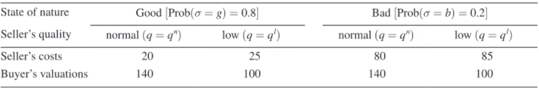
Table 1—Experimental Parameters
State of nature Good [Prob(σ= g)= 0.8] Bad [Prob(σ= b)= 0.2]
Seller’s quality normal (q = q n) low (q = q l ) normal (q = q n) low (q = q l )
Seller’s costs 20 25 80 85
Buyer’s valuations 140 100 140 100
Notes: The table summarizes the main parameters of the experiment. Buyers’ valuations for the product and sellers’ production costs are displayed for both states of nature and both quality levels available to the seller.
The lower bound of the price range is determined in an auction in such a way that pl∈[35, 75], the same interval as for the fixed price in rigid contracts.
Step 3: The sellers’ contract auction
When both buyers in an interaction group have chosen their contract type, the two contracts are auctioned off to the sellers. The sequence of the auctions is randomly determined within each group. In both cases the auction starts off at 35 and then increases by one unit every half second. Each of the two sellers has a button that allows him to accept the contract at any time during the auction. Thus, the first seller who is willing to accept the displayed fixed price or the displayed lower price bound respectively gets the contract. The seller who loses the auction and does not get the contract realizes the outside option xs.
Date 1: Trade
Step 4: Determination of the state of nature
After the contracts have been auctioned off to the sellers, a computerized random device determines the state of nature for each contract independently. Both sellers and buyers observe the realized state for their contracts and are informed whether a mutually beneficial transaction can take place or not. Trade can always take place when the buyer has chosen a flexible contract, because the price range allows the buyer to choose prices that cover the seller’s cost in both states of nature. In the case of a rigid contract, in contrast, trade occurs only in the good state. In the bad state the fixed price is always lower than the seller’s cost, and a mutually beneficial trans-action is not feasible. If trade does not occur, the buyer and the seller realize their outside options (xB and xs).
Step 5: The buyer’s price choice
Once the state has been revealed, the buyer determines the actual trading price. In a rigid contract the buyer does not have a choice, since the price has been fixed at date 0. In a flexible contract, the buyer can choose the price. In the good state the buyer can choose any price p ∈[ pl, 140]. In the bad state the buyer has to make sure that the price is such that the seller cannot make losses, i.e., he must choose a price p∈[c(q l, b)+ x
s , v(q h)]=[95, 140].5
Step 6: The seller’s quality choice
Sellers observe the price choice of their buyer and then determine their quality. In both types of contracts the sellers have the choice between normal (q n) and low (q l ) quality. Remember that choosing low instead of normal quality increases the seller’s cost by 5 units irrespective of the contract type and realized state of nature (see Table 1).
Step 7: Profit calculations
After the quality choice of sellers all decisions have been made. Profits are calcu-lated and displayed on subjects’ screens.
5 Again we do not allow prices to be such that the seller can make losses by choosing low quality, since we want
Step 8: Market information for the buyers
Subsequent to viewing the profit screen buyers also get some aggregated infor-mation about the market outcome. Specifically, they are informed about profits of buyers in both contract types averaged over all past periods. Furthermore, they learn how many buyers have chosen the rigid contract and the flexible contract in the cur-rent period.6
The screen with the market information for buyers ends the period. After this a new period begins and the participants are randomly reassigned to a new interaction group.
Remark: We have ruled out lump sum transfers and restricted flexible contracts to
those in which the buyer chooses the price ex post. We discuss this further in IIIB. B. Experimental Robustness Checks
We provide two experimental robustness checks.
Reduced Flexibility.—Our baseline treatment compares completely rigid contracts with maximally flexible contracts: the upper bound in the price range is exogenously fixed at the buyers’ maximal willingness to pay, ph= v(q h )= 140. Studying these extreme cases gives us the best chance of illustrating the trade-off between rigidity and flexibility. However, the buyers would prefer a contract with less flexibility: the price never needs to go above p = c(ql, b)+ x
s= 95 in order to permit trade in the bad state, and, according to Hart and Moore (2008), a lower upper bound should reduce aggrievement and shading. In fact with an upper bound of 95, buyers with a flexible contract have only one price available in the bad state of nature, p = 95, and there should be no aggrievement at all. In our reduced flexibility treatment we replace the upper bound of 140 in the flexible contract with 95.
No Competition.—As noted in the introduction, Hart and Moore (2008) argue that competition will provide objectivity to the contract terms, and parties will there-fore perceive the initial contract to be fair. Of course, it is possible that parties will perceive a contract to be fair even if it is not negotiated under competitive condi-tions. In the no competition treatment we see whether this is the case.
The interaction between buyers and sellers takes place in the same way as in the baseline treatment except for the determination of the contract terms at date 0 (i.e., the fixed price in rigid contracts and the lower bound in flexible contracts). As in the base-line treatment the first step is that the buyer chooses his contract type. However, while the baseline treatment subsequently relies on competitive auctions, the contract terms in the no competition condition are determined by an exogenous random device. The random device draws the terms out of the distribution of auction outcomes generated by the baseline treatment. This guarantees that any behavioral changes between the baseline and the no competition treatments are driven by the difference in the determi-nation of contract terms and not by differences in the contract terms themselves. After
6 The aim of the provision of this information was to make learning easier for buyers. Since our set-up allows
for many possible constellations (two contract types, two states of nature, two quality levels, many prices), learning from individual experience is rather difficult.
the contract terms have been set for both buyers in an interaction group, each contract is randomly (and independently) assigned to one of the two sellers (i.e., as in the base-line treatment each seller can end up with zero, one, or two contracts).
C. subjects, payments, and procedures
All subjects were students of the University of Zurich or the Swiss Federal Institute of Technology Zurich (ETH). Economists and psychologists were excluded from the subject pool. We used the recruitment system ORSEE (Ben Greiner 2004). Each subject participated in only one session. Subjects were randomly subdivided into two groups before the start of the experiment; some were assigned the role of buyers and others the role of sellers. The subjects’ roles remained fixed for the whole ses-sion. All interactions were anonymous, i.e., the subjects did not know the personal identities of their trading partners.
To make sure that subjects fully understood the procedures and the payoff conse-quences of the available actions, each subject had to read a detailed set of instruc-tions before the session started. Participants then had to answer several quesinstruc-tions about the feasible actions and the payoff consequences of different actions. We started a session only after all subjects had correctly answered all questions. The exchange rate between experimental currency units (“points”) and real money was 15 Points = 1 Swiss Franc (~US $ 0.83, in summer 2007).
In order to make the sellers familiar with the auction procedure in the baseline treatment and the reduced flexibility treatment we implemented two trial auctions— one with a rigid contract and one with a flexible contract—before we started the actual experiment. In the trial phase each seller had his own auction, i.e., they did not compete with another seller and no money could be earned.
The experiment was programmed and conducted with z-Tree (Fischbacher 2007). We conducted five sessions of the baseline treatment, two sessions of the reduced flexibility treatment, and five sessions of the no competition treatment. We had 28 subjects (14 buyers and 14 sellers) in ten of our 12 sessions and—owing to no-shows—24 subjects (12 buyers and 12 sellers) in the remaining two sessions. This yields a total number of 328 participants in the experiment. A session lasted approx-imately two hours, and subjects earned on average 59 Swiss Francs (including a show up fee of 10 Swiss Francs).
II. Behavioral Predictions
In this section we derive the predictions for our experiment and discuss some design features.
A. predictions under pure self-Interest
If we assume common knowledge of rationality and money-maximizing behavior, the predictions for the baseline treatment of our experiment are straightforward.7
7 We do not believe that these assumptions provide an accurate description of our participants’ behavior.
Since shading on performance is costly, purely selfish sellers provide normal quality irrespective of the realized price in both types of contracts. Buyers anticipate sellers’ behavior and choose the lowest price allowed by the contract. In the contract auc-tions rivalry between sellers implies that the fixed price in rigid contracts, respec-tively the lower price bound in flexible contracts, ends up at the competitive level, i.e., pr = 35 and pl = 35.8 Accordingly, when buyers choose their contract types they anticipate the following outcomes: in the good state of nature both contract types deliver the same outcome
(
πB= v(q n)− p = 140 − 35 = 105)
, but in the bad state of nature the flexible contract is more attractive, because it allows for trade(
πB= v(q n )− p = 140 − 95 = 45), while the rigid contract leads to the realization of the outside option (πB= xB= 10). This implies that buyers always choose the flexible contract.The predictions for our two robustness checks are equally simple. The reduced flex-ibility condition and the no competition treatment should lead to the same outcome as the baseline condition. As long as the upper bound is high enough to allow for trade in the bad state ( ph≥ 95), changing the upper bound does not affect the arguments given above. Since the contract terms will be identical to the terms realized in the baseline condition, eliminating competition at date 0 should also not change anything.
We summarize the prediction of the standard economic model as the standard Hypothesis:
(i) Market forces imply that the fixed price in rigid contracts and the lower bound of the price range in flexible contracts end up at the competitive level, i.e., pr= pl= 35.
(ii) Sellers never choose low quality irrespective of the contract type and price level. Buyers always choose the lowest price available in flexible contracts. (iii) Buyers’ profits are higher in flexible contracts than in rigid contracts.
Therefore, buyers prefer flexible contracts.
(iv) Lowering the upper bound in flexible contracts does not change outcomes. (v) Eliminating ex ante competition does not change outcomes.
B. predictions if Contracts are Reference points
According to Hart and Moore (2008), an ex ante contract, negotiated under com-petitive conditions, shapes parties’ entitlements regarding ex post outcomes. In Hart and Moore (2008), a party compares the ex post outcome to the most favorable outcome permitted by the contract, and if he does not get what he feels entitled to he is aggrieved and shades on noncontractible aspects of performance. In the Appendix
these predictions provide an important benchmark.
8 Remember: Since p = 35 corresponds to p = c(q l, g)+ x
s and the seller must offer at least p = c(q l, b)+ xs= 95 in the bad state of nature, a seller can never be worse off if he accepts a contract than if he accepts his outside option.
we extend Hart and Moore (2008) to allow for the case where parties may feel enti-tled to an outcome other than the most favorable outcome. The model’s predictions are broadly similar to Hart and Moore (2008). Rigid contracts pin down outcomes, sellers get what they expect, and so sellers are not aggrieved. Accordingly, shading should not occur in rigid contracts. However, in a flexible contract, the seller may be aggrieved and shade if he gets a lower price than he had hoped for. We show that the heterogeneity in seller entitlements implies that the frequency of shading is decreas-ing in price. Given this the buyer will either increase the price in flexible contracts to avoid shading or accept the possibility of getting low quality. Thus, although the flexible contract guarantees trade in both states, the reference dependent behavior of sellers has a negative impact on the buyers’ profit. Hence flexible contracts may be less profitable than rigid contracts. Reference dependent behavior does not, how-ever, change the auction outcome: rivalry between sellers still ensures that the lower bound of the price range in flexible contracts, and the fixed price in rigid contracts, is 35. (Recall that we do not allow the price to fall below 35; see footnote 4.)
The assumption that contracts act as reference points also suggests that our exper-imental robustness checks should have an impact on trading parties’ behavior. With the upper bound of the price range in flexible contracts reduced from 140 to 95, buy-ers have only one price available in the bad state of nature ( p= 95), and so sellers should not be aggrieved, and there should be no shading. In addition, decreasing the upper bound may also lower (some) sellers’ reference prices and decrease shading in the good state of nature in flexible contracts.9 As a consequence, flexible contracts may be more profitable, and the buyers may therefore choose the flexible contract more often than in the baseline treatment.
Eliminating ex ante competition is also predicted to have an effect. In the absence of ex ante competition low prices in rigid contracts are no longer justified by competi-tive market forces at date 0, and so we expect to see more shading in rigid contracts.
These considerations lead to the Reference point Hypothesis:
(i) Market forces imply that the fixed price in rigid contracts and the lower bound of the price range in flexible contracts end up at the competitive level, i.e., pr= pl= 35.
(ii) In rigid contracts sellers never choose low quality irrespective of the price level. In flexible contracts sellers’ quality provision is price dependent. Heterogeneity in seller entitlements implies that the frequency of shading is decreasing in the price. Given the price dependence of quality, buyers may not choose the lowest price available in flexible contracts.
9 Lowering the upper bound may affect reservation prices in the good state in two ways: (i) When the upper
bound is high ( ph= 140), some sellers may have reference prices above 95. Lowering the upper bound reduces these reference prices to 95. We assume that sellers never hope for a price outside the contract. (ii) Lowering the upper bound may also affect reference prices of sellers who hope for a price of less than 95, when the upper bound is high. This is the case if reference prices are a function of the bounds of the price range. Our formal analysis in the Appendix allows for this possibility, since we assume that the reference price is a function of the contract type.
(iii) Buyers’ profits in flexible contracts are lower than predicted by the standard model. If the impact of the reference dependent preferences is strong, buyers may even make higher profits in rigid contracts than in flexible contracts. (iv) Lowering the upper bound of the price range leads to less shading in flexible
contracts, in particular in the bad state of nature.
(v) Eliminating ex ante competition increases shading in rigid contracts. C. discussion of design Features
It is important to emphasize that the aim of this paper is not to determine whether people succeed in choosing an optimal contract. We are interested rather in the more fundamental question of whether the underlying behavioral assumptions of the Hart-Moore model are empirically relevant. To study this question in a clean and controlled way, we have intentionally abstracted from some theoretical features of the model. In this section we discuss to what extent the simplifications in our experi-mental set-up affect our predictions.
We have supposed that only the seller can shade, and that the buyer’s value is certain. In the Hart-Moore model either of these simplifications implies that the first-best can be achieved.10 In other words, the trade-off between contractual flex-ibility and rigidity is destroyed. However, since optimality of contracts is not the focus of this study, we avoid this problem by restricting the set of feasible contracts. Specifically, we exclude lump sum transfers and consider only contracts in which the buyer chooses the ex post price.
Another important simplification and limitation is that we have not allowed the parties to write informal state contingent contracts. For example, the buyer and seller could agree that price will depend on the seller’s realized cost, which is observed by both parties. Hart and Moore (2008) discuss informal contracts of this kind. They argue that such contracts may be problematic in situations where there is a little bit of asymmetric information and the parties exhibit self-serving biases. Under these conditions, each party may be able to convince himself that the state is favorable to him. This is likely to lead to aggrievement and shading, as in the flexible contracts studied in this paper. Obviously, a considerably more complicated experiment would be required to test the role of informal state contingent contracts in the presence of asymmetric information and self-serving biases. We leave this for future work.
Hart and Moore (2008) assume that trading parties are indifferent between per-functory and consummate performance, i.e., shading is neither costly nor beneficial. However, they emphasize that assuming indifference is just a technically convenient 10 On the one hand, if the buyer’s value is certain, a buyer can offer a rigid contract with the fixed price equal to
v(qn ). Trade will occur in both states, there will be no aggrievement since there is only one price, and sellers will provide normal quality. Redistribution of surplus from sellers to buyers (because of competition) can be achieved through lump sum payments conditional on winning the contract auction. On the other hand, if the buyer’s value is uncertain but only sellers can shade, a buyer can offer a flexible contract in which the seller has the right to choose the price ex post. Sellers will choose a price equal to the buyer’s realized value of v(q n), and since the sellers get their most favorable outcome they will not shade; also by assumption buyers cannot shade. Redistribution of sur-plus from sellers to buyers (because of competition) is again achieved through lump sum payments conditional on winning the auction.
way to capture the idea that the cost of providing low quality is not substantially higher or lower than the cost of providing normal quality. With regard to the aim of our paper, implementing strict indifference between shading and normal per-formance in the experiment would be problematic. The reason is that indifference would not rule out equilibrium shading under standard economic assumptions in our set-up. In order to make sure that shading cannot be explained if people are motivated by pure self-interest, we implemented costly shading. However, since the increase in the sellers’ costs is low
(
c(q l, σ)− c(q n, σ)= 5)
relative to the damage which shading imposes on the buyer(
v(q n)− v(q l )= 40)
, our set-up is still in line with the spirit of the model.11It is obvious that the probabilities with which the two states of nature occur are decisive for the relative attractiveness of rigid and flexible contracts. Since we intend to study the impact of contract types on behavior, we need a sufficient number of observations for flexible and rigid contracts. The rigid contract is attractive only if the disadvantage due to the nonexistence of trade in the bad state of nature is not too large. We therefore decided that the good state of nature should occur with a high probability (w g= 0.8).12
III. Results
In this section we present and discuss our results. The analysis of our data at the aggregate level in Section IIIA reveals that the outcomes largely confirm the refer-ence point hypothesis and contradict the predictions of standard economic theory. In Section IIIB we demonstrate how our findings can be explained in light of the differences in the price dependence of sellers’ performance across the two contract types. Sections IIIC and IIID illustrate that the predictions of the reference point theory are also relevant for individual behavior of sellers and buyers. In Section IIIE we discuss the results of our robustness checks.
A. Aggregate Findings
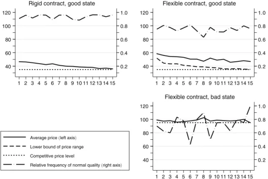
Table 2 and Figure 1 summarize the main results for our baseline treatment. Table 1 presents averages of prices, quality choices, auction outcomes, profits, and contract choices for rigid and flexible contracts in the good and bad state of nature. Figure 1 displays the development of prices and quality choices over time.
Auction Outcomes in Rigid and Flexible Contracts.—Figure 1 illustrates the power of competition in the auction phase of our experiment. The fixed price in rigid 11 Alternatively we could have chosen to make the provision of low quality slightly less costly than the
provi-sion of normal quality. However, the case of costly shading probably leads to stronger effects. It seems more likely that aggrievement triggers costly shading than that the absence of aggrievement causes people to engage in costly voluntary cooperation. The reason is that aggrievement certainly causes a negative sentiment, while the absence of aggrievement may be completely neutral and may not imply the positive sentiment necessary to induce costly cooperation. Of course, this remains an empirical question that should be addressed in future work.
12 Another way to make sure that we have a sufficient number of observations in both contract types would
have been to assign contract types exogenously. However, this would have changed the spirit of the experiment in a fundamental way. From the perspective of the seller, it certainly makes a big difference whether the buyer himself chooses to limit his ability to adjust the price ex post or whether this is imposed by the experimenter (see the discus-sion in Section IV).
contracts and the lower price bound in flexible contracts converge to the competi-tive price of 35 over time. In the final period the auctions deliver an average fixed price of 35.7 and an average lower bound of 35.2. Because auction outcomes are somewhat higher in the early period of the experiment the overall averages of both the fixed price in rigid contracts and the lower bound of the price range in flexible contracts are slightly above the predicted level of 35. Both averages turn out to be about 40 (see Table 2). A nonparametric signed rank test using session averages as observations confirms that the auction outcomes for rigid contracts and flexible contracts are not significantly different.13
prices and Quality in Rigid and Flexible Contracts.—The fact that auction out-comes do not differ across contract types implies that, in principle, the buyers have the possibility to pay the same prices in both types of contracts when the good state of nature is realized. However, if the reference point hypothesis is correct, buyers in flexible contracts may have the incentive to increase their prices above the lower price bound, because low prices may cause sellers to be aggrieved and lead to shad-ing. This is in fact what we observe. In 75 percent of the flexible contracts in which the good state has been realized, buyers pay a price which is strictly above the lower bound of the price range determined in the auction. Although the lower price bound is only about 40 on average, the average price level is 51 (see Table 2). This difference between the actual price paid by the buyer and the lower bound of the price range is very stable and does not disappear over time (see Figure 1). In rigid contracts, in contrast, the final price at date 1 is equal to the fixed price which has been determined in the auction at date 0. We have already shown above that these 13 The session averages for the fixed price in rigid contracts are: 37.3, 40.7, 40.5, 41.2, and 43.4. The session
averages for the lower bound of the price range in flexible contracts are: 37.5, 41.6, 40.5, 38.8, and 43.4. Table 2—Summary of Outcomes in Rigid and Flexible Contracts (Baseline)
Contract type Rigid contract Flexible contract
State of nature Good Bad Good Bad
Average price 40.7 — 51.1 98.4
Relative frequency of normal quality 0.94 — 0.75 0.70
Average auction outcome 40.7 40.2
Average profit buyer (per state) 96.8 10 78.9 29.7 Average profit seller (per state) 20.4 10 29.8 16.9 Average profit buyer (over both states) 77.9 68.9 Average profit seller (over both states) 18.1 27.2
Relative frequency of contract 0.50 0.50
Notes: The table summarizes the outcomes for rigid and flexible contracts in both states of nature. All numbers are based on the data of all 5 sessions. Average price is the average of the trading price and Relative frequency of normal quality measures how often the seller has chosen the normal quality. For rigid contracts this information is available only for the good state, because trade does not occur in the bad state. Average auction outcome is the average of the fixed price in case of rigid contracts and the lower bound of the price range in case of flexible contracts. Average profit buyer (seller)(per state) measures the average payoff of buyers (sellers) for each state and contract. In rigid contracts the payoffs in the bad state of nature are the outside options of the market participants. Average profit buyer (over both states) is the overall average payoff of buyers (sellers) for each contract type. Relative frequency of contract is the share of the total number of contracts that corresponds to each contract type.
prices are around 40 on average and converge to the competitive level of 35 over time.14 This implies that in the good state buyers pay on average substantially higher prices in flexible contracts than in rigid contracts. A nonparametric signed rank test confirms that the price difference between rigid and flexible contracts is statistically significant
(
p-value = 0.031 (one-sided))
.15Although prices are close to the competitive level, shading is almost absent in rigid contracts. Sellers provide normal quality in 94 percent of the cases in which the good state is realized. In flexible contracts, however, the higher prices are not always suffi-cient to prohibit sellers from shading. In the good state sellers provide normal quality in only 75 percent of the cases (see Table 2). The difference in the frequency of shad-ing between the two contract types is statistically significant
(
nonparametric signed rank test, p-value = 0.031 (one-sided))
and very stable over time (see Figure 1).16payoffs and Contract Choice.—The differences in price and quality levels have important implications for payoffs of buyers and sellers in the good state of nature. Since prices are higher and quality is lower in flexible contracts, buyers earn, on aver-age, considerably lower payoffs in flexible contracts (78.9) than in rigid contracts
14 The “auction outcome” in Table 2 is the average of the fixed prices in all rigid contracts. The “price” in Table 2
and Figure 1, in contrast, is the average of the fixed prices in all rigid contracts in which trade occurred. However, since the state of nature is randomly determined, there is no systematic difference between the two.
15 The session averages for the price in rigid contracts are: 37.3, 40.8, 40.8, 41.0, and 43.4. The session averages
for the price in flexible contracts are: 51.7, 49.7, 49.0, 50.2, and 54.0.
16 In the good state the session level frequencies of high quality in rigid contracts are (in percent): 89, 97, 95, 91,
and 96. The corresponding numbers for flexible contracts are (in percent): 78, 76, 79, 67, and 75.
0.2 0.4 0.6 0.8 1.0
0.2 0.4 0.6 0.8 1.0
0.2 0.4 0.6 0.8 1.0 40
60 80 100 120
40 60 80 100 120
40 60 80 100 120
1 2 3 4 5 6 7 8 9 10 11 12 13 14 15 1 2 3 4 5 6 7 8 9 10 11 12 13 14 15
1 2 3 4 5 6 7 8 9 10 11 12 13 14 15
Rigid contract, good state Flexible contract, good state
Flexible contract, bad state
Average price (left axis)
Lower bound of price range Competitive price level
Relative frequency of normal quality (right axis)
(96.8). The opposite is true for sellers. Although the higher frequency of shading increases sellers’ costs in flexible contracts, the price difference is large enough to offset this. While the average payoff of sellers in flexible contracts is 29.8, their payoff in rigid contracts is 20.4 (see Table 2). Both payoff differences are highly significant according to nonparametric signed rank tests
(
Sellers: p-value = 0.031 (one-sided), Buyers: p-value = 0.031 (one-sided))
.17In the bad state of nature rigid contracts do not allow for trade. Accordingly, buy-ers and sellbuy-ers realize their outside options. In flexible contracts trade takes place and buyers must offer a price of at least 95. We observe that buyers pay on average a price of 98.4 (see Table 2). Thus, while average prices are substantially higher than the lower price bound in the good state, prices in the bad state are very close to the minimal price buyers can offer. In response shading is slightly more frequent in the bad state than in the good state. However, a nonparametric signed rank test shows that this difference is not statistically significant.18 We will later investigate whether the price setting strategies of buyers in flexible contracts reflect profit maximizing behavior. Since outside options generate a payoff of only 10, sellers and buyers are better off with a flexible contract in the bad state of nature. Average payoffs are 29.7 for buyers and 16.9 for sellers, respectively (see Table 2).
We have established that buyers indeed face a trade-off between rigidity and flexibility. Given the stronger tendency for shading in flexible contracts, rigid con-tracts are more attractive in the good state of nature. However, since fixed prices prohibit trade when costs are high, having a flexible contract is of advantage in the bad state of nature. But which contract is more profitable in total? It turns out that overall the need to pay higher prices and the higher frequency of shading are strong enough to render flexible contracts less profitable for buyers than rigid con-tracts. While the average buyer payoff is 77.9 in rigid contracts, it is only 68.9 in flexible contracts. This difference is statistically significant
(
nonparametric signed rank, p-value = 0.031 (one-sided))
.19 Sellers, in contrast, are better off in flexible contracts. Average seller payoffs in rigid contracts are 18.1, compared to 27.9 in flexible contracts. Also this difference is statistically significant(
nonparametric signed rank, p-value = 0.031 (one-sided))
.20 The finding that rigid contracts yield higher profits for buyers than flexible contracts is, of course, highly dependent on the choice of parameters. It is certainly easy to find other parameter constellations which yield the opposite results (e.g., higher probability for bad state, weaker impact of shading on buyer’s value, etc.). However, our findings illustrate not only that a trade-off between contractual flexibility and rigidity exists, but also that there are parameters under which this trade-off has strong consequences for economic outcomes.17 The session averages for buyer profits in the good state are: 98.3, 97.9, 97.4, 95.3, 95.0 (rigid contracts) and
79.3, 80.6, 82.8, 76.6, 76.0 (flexible contracts). The session averages for seller profits in the good state are: 16.8, 20.6, 20.5, 20.6, 23.2 (rigid contracts) and 30.6, 28.5, 28.0, 28.6, 32.8 (flexible contracts).
18 In the bad state of nature the session level frequencies of high quality in flexible contracts are (in percent):
70, 46, 83, 58, and 83.
19 The session averages for buyer payoffs in rigid contracts are: 80.1, 80.1, 78.8, 75.0, and 75.3. The session
averages for buyer payoffs in flexible contracts are: 71.0, 69.9, 71.4, 65.3, and 67.2.
20 The session averages for seller payoffs in rigid contracts are: 15.4, 18.4, 18.3, 18.1, and 20.1. The session
In contrast to the standard prediction, buyers choose rigid contracts in 50 percent of the cases (see Table 2). If we look at the development over time, we observe that the share of rigid contracts has an upward tendency. It starts off at 38 percent in period 1 and ends up at 56 percent in period 15. An OLS regression of the fraction of rigid contracts on periods indicates that this positive time trend is statistically significant.21
B. sellers’ Quality Choice:
Contract-dependent price-Quality Relationships
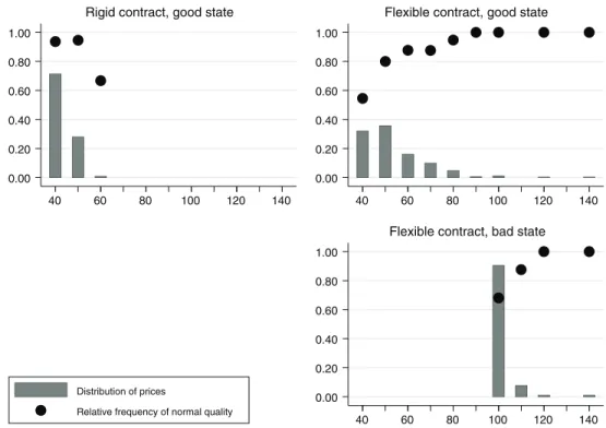
The discussion of Table 2 and Figure 1 has shown that in the aggregate our find-ings support the reference point hypothesis. Next, we analyze whether the underly-ing behavioral patterns are also in line with the assumption that contracts provide reference points for trading relationships. We start with sellers’ performance choices. Figure 2 displays the relative frequency of normal quality conditional on the price paid by the buyer for each contract type and both states of nature. In addition, the figure shows the relative frequency with which each price level is chosen by buyers. Notice that prices on the horizontal axis are rounded to the nearest multiple of ten. The figure provides strong support for the seller behavior predicted by the reference point hypothesis. In rigid contracts sellers almost always choose normal quality even if prices are very close to the competitive level. There is no noteworthy cor-relation between prices and the frequency of normal quality.22 For flexible contracts, in contrast, the figure suggests a strong positive correlation between prices and the willingness to provide normal quality in both states of the world. If prices are close to the competitive level in the good state of nature, normal quality is chosen in less than 60 percent of the contracts. The frequency of normal quality is clearly increas-ing in price, but in order to reach the same average quality as observed in rigid contracts, buyers must raise their price to a level of at least 75. In the bad state of nature prices close to the lowest possible level also trigger a lot of shading. At prices between 95 and 104 sellers provide normal quality in less than 70 percent of the contracts. Also in the bad state substantial price increases are necessary to reach a high quality level on average.
We provide statistical backup for our observations on price dependence of quality with a regression analysis in Table 3. In the first column of the table we investigate the good state of nature. We regress an indicator variable for choosing normal qual-ity on price increments, an indicator variable for flexible contracts, and the inter-action term of the two. We define price increments as the difference between the actual price and the competitive price of 35. Using price increments instead of prices allows us to interpret the constant as the frequency with which sellers provide high quality when buyers offer the competitive price of 35 in rigid contracts. The constant of 0.94 therefore reflects that prices close to the competitive level do not trigger much shading in rigid contracts. Furthermore, the coefficient of price increments is 21 The regression uses one observation per period and session. The dependent variable is the fraction of rigid
contracts; the explanatory variable is period. The estimated coefficients are as follows: Constant = 0.43, p-value <
0.001; Period = 0.010, p-value = 0.002 ( p-values are based on robust standard errors).
22 The low frequency of normal quality when prices are around 60 should be ignored, because it is based on a
close to zero and insignificant, indicating that sellers’ quality choices in rigid con-tracts do not depend on prices in a statistically significant way. The situation is very different in flexible contracts. The significantly negative coefficient of the dummy for flexible contracts shows that if prices are at the competitive level sellers are much more likely to choose low quality in flexible contracts than in rigid contracts (−0.34, p-value < 0.01). The regression also confirms the statistical significance of the positive impact of higher price increments on sellers’ quality choices in flexible contracts (F-test: price increment + price incr. × flex. contr. = 0, p-value < 0.01).23 In column 2 we show that a probit estimation (marginal effects reported) using the same set of variables yields results similar to the ones of the linear probability model used in column 1. Column 3 investigates the bad state of nature. We regress the indi-cator variable for choosing normal quality on price increments (now defined as the difference between price and the lowest possible price of 95). The constant indicates that the frequency of normal quality is only 0.66 when buyers pay the lowest pos-sible price in the bad state of nature. In addition, the significant coefficient confirms that there is also a significant impact of price increments on quality in the bad state of nature. Column 4 documents that a probit estimation yields similar results ( mar-ginal effects reported).
23 Since the lower bound of the price range is not always equal to the competitive price, one might suspect that
the realized lower bound could be relevant for the seller’s quality choice. For example, the seller could evaluate the generosity of the price paid by the buyer relative to the lower bound of the available price range. However, a regression of quality on price increments and the lower bound of the price range reveals that this is not the case. The coefficient for the lower bound of the price range is close to zero and not significant.
0.00 0.20 0.40 0.60 0.80 1.00
0.00 0.20 0.40 0.60 0.80 1.00
0.00 0.20 0.40 0.60 0.80 1.00
40 60 80 100 120 140 40 60 80 100 120 140
40 60 80 100 120 140
Rigid contract, good state Flexible contract, good state
Flexible contract, bad state
Distribution of prices
Relative frequency of normal quality
C. Individual seller Behavior: Quality Choice within and across Contracts The analysis of sellers’ behavior in Figure 2 and Table 3 is based on pooled data from all sellers in the experiment. However, the reference point hypothesis relies on behavioral assumptions about preferences and makes specific predictions regarding individual behavior of sellers in rigid and flexible contracts. Since contract assignment is endogenous in the experiment, our analysis hitherto does not provide evidence that our aggregate findings are the consequence of different behavior of the same sellers in different types of contracts. It could also be that the aggregate effects are the con-sequence of self-selection of distinct seller groups into different contract types. For example, the result that shading is more frequent in flexible contracts than in rigid contracts would also be observed if those sellers who self-select into flexible contracts are systematically more likely to provide low quality than those sellers who self-select into rigid contracts. In the following we dig deeper and examine whether sellers accept both types of contracts, and if so, how their behavior differs across contract types.
In Figure 3 we show the distribution of rigid and flexible contracts over indi-vidual sellers in the experiment. We observe that most sellers do not self-select into a specific type of contract, i.e., most sellers conclude several rigid as well as several flexible contracts. Specifically, the figure reveals that every seller has experienced each contract type at least once and for most sellers there are multiple observations for each contract type (84 percent of sellers have experienced at least four contracts of each type). Furthermore, even if we consider only contracts in which trade actu-ally occurred, we still have at least one observation for each seller and contract type. This implies that each seller has made at least one quality decision in each type of contract, and so we can compare sellers’ performance choices across contract types.
Table 3—Price Dependence of Quality Across Contract Types (Baseline)
Dependent variable Quality [σ= g] Quality [σ= b]
OLS Probit [ME] OLS Probit [ME]
(1) (2) (3) (4)
Price increment 0.000 0.000 0.013* 0.023***
[0.002] [0.004] [0.005] [0.009]
Flexible contract −0.335*** −0.298***
[0.060] [0.060] Price increment × flex 0.009* 0.009*
[0.004] [0.005]
Constant 0.936*** 0.657
[0.025] [0.075]
Observations 805 805 104 104
R2 0.13 0.03
Notes: price increment is defined as price minus 35 in columns 1 and 2 and as price minus 95 in columns 3 and 4. Flexible contract is an indicator variable which is unity if the contract is of the flexible type and zero otherwise. price increment × flex is the interaction term of price increment and flexible contract. Columns 1 and 3 report coef-ficients of OLS estimations. Columns 2 and 4 report marginal effects based on probit estimations. Since observa-tions within sessions may be dependent all reported standard errors are adjusted for clustering at the session level.
*** Significant at the 1 percent level. ** Significant at the 5 percent level. * Significant at the 10 percent level.
In Table 4 we analyze individual behavior in detail. According to the reference point hypothesis sellers may shade on performance in flexible contracts but never in rigid contracts. We find that 51 of the 68 sellers in our experiment exhibit a behav-ioral pattern which is consistent with this prediction. Twenty-seven of these 51 sellers do not provide low quality in either contract type (first column), while the other 24 sellers provide low quality in some of their flexible contracts (second col-umn). Notice: While the behavior of sellers who do not shade on performance at all can also be explained by standard economic theory (see the standard prediction in Section IIA), this behavior does not contradict the reference point hypothesis. If a seller happens to receive offers above his threshold price whenever he concludes a flexible contract, it is plausible that he never shades on performance. Since sellers do not indicate their threshold price in our experiment, we cannot compare the thresh-old prices of sellers across differently behaving groups. However, Table 4 shows that sellers who never provide low quality have concluded a lower number of flexible contracts and receive, on average, higher price offers in these contracts (especially in the good state of nature). These two factors make it less likely that a seller with a given feeling of entitlement engages in shading.
The remaining 17 sellers in our experiment exhibit behavior which is not consis-tent with the reference point hypothesis, i.e., they provide at least once low quality in a rigid contract (see third and fourth column in Table 4). A closer look reveals that seven of these sellers show behavioral patterns which are “almost in line” with the prediction of the reference point hypothesis: they provide low quality exactly once in a rigid contract, and they shade more often in flexible contracts than in rigid con-tracts, in both absolute and relative terms. Only ten of our 68 sellers make decisions which are clearly not in line with the reference point hypothesis.
In addition, the reference point hypothesis also suggests a positive (or zero) corre-lation of prices and quality in flexible contracts for each individual seller. However,
0 2 4 6 8 10 12 14 16
Number of rigid contracts
0 2 4 6 8 10 12 14 16
Number of flexible contracts