Straggling Servers
Downloaded from: https://research.chalmers.se, 2019-09-07 22:09 UTC
Citation for the original published paper (version of record):
Severinson, A., Graell i Amat, A., Rosnes, E. (2019)
Block-Diagonal and LT Codes for Distributed Computing With Straggling Servers
IEEE Transactions on Communications, 67(3): 1739-1753
http://dx.doi.org/10.1109/TCOMM.2018.2877391
N.B. When citing this work, cite the original published paper.
research.chalmers.se offers the possibility of retrieving research publications produced at Chalmers University of Technology. It covers all kind of research output: articles, dissertations, conference papers, reports etc. since 2004.
research.chalmers.se is administrated and maintained by Chalmers Library
Block-Diagonal and LT Codes for Distributed
Computing With Straggling Servers
Albin Severinson,
Student Member, IEEE
, Alexandre Graell i Amat,
Senior Member, IEEE
,
and Eirik Rosnes,
Senior Member, IEEE
Abstract—We propose two coded schemes for the distributed computing problem of multiplying a matrix by a set of vectors. The first scheme is based on partitioning the matrix into submatrices and applying maximum distance separable (MDS) codes to each submatrix. For this scheme, we prove that up to a given number of partitions the communication load and the computational delay (not including the encoding and decoding delay) are identical to those of the scheme recently proposed by Li et al., based on a single, long MDS code. However, due to the use of shorter MDS codes, our scheme yields a significantly lower overall computational delay when the delay incurred by encoding and decoding is also considered. We further propose a second coded scheme based on Luby Transform (LT) codes under inactivation decoding. Interestingly, LT codes may reduce the delay over the partitioned scheme at the expense of an increased communication load. We also consider distributed computing under a deadline and show numerically that the proposed schemes outperform other schemes in the literature, with the LT code-based scheme yielding the best performance for the scenarios considered.
Index Terms—Block-diagonal coding, computational delay, decoding delay, distributed computing, Luby Transform codes, machine learning algorithms, maximum distance separable codes, straggling servers.
I. INTRODUCTION
Distributed computing systems have emerged as one of the most effective ways of solving increasingly complex computa-tional problems, such as those in large-scale machine learning and data analytics [1]–[3]. These systems, referred to as “warehouse-scale computers” (WSCs) [1], may be composed of thousands of relatively homogeneous hardware and software components. Achieving high availability and efficiency for applications running on WSCs is a major challenge. One of the main reasons is the large number of components that may ex-perience transient or permanent failures [3]. As a result, several This work was presented in part at the IEEE Information Theory Workshop (ITW), Kaohsiung, Taiwan, November 2017, and it was published in part in “Coding for Distributed Computing: Investigating and improving upon coding theoretical frameworks for distributed computing,” MSc. thesis, Chalmers University of Technology, June 2017. This work was funded by the Swedish Research Council under grant 2016-04253 and the Research Council of Norway under grant 240985/F20.
Albin Severinson was with the Department of Electrical Engineering, Chalmers University of Technology, SE-41296 Gothenburg, Sweden. He is now with Simula UiB and the Department of Informatics at the University of Bergen, N-5020 Bergen, Norway (email: [email protected]).
Alexandre Graell i Amat is with the Department of Electrical Engineering, Chalmers University of Technology, SE-41296 Gothenburg, Sweden (email: [email protected]).
Eirik Rosnes is with Simula UiB, N-5020 Bergen, Norway (email: [email protected]).
distributed computing frameworks have been proposed [4]–[6]. In particular, MapReduce [4] has gained significant attention as a means of effectively utilizing large computing clusters. For example, Google routinely performs computations over several thousands of servers using MapReduce [4]. Among the challenges brought on by distributed computing systems, the problems of straggling servers and bandwidth scarcity have recently received significant attention. The straggler problem is a synchronization problem characterized by the fact that a distributed computing task must wait for the slowest server to complete its computation, which may cause large delays [4]. On the other hand, distributed computing tasks typically require that data is moved between servers during the com-putation, the so-calleddata shuffling, which is a challenge in bandwidth-constrained networks.
Coding for distributed computing to reduce the computa-tional delay and the communication load between servers has recently been considered in [7], [8]. In [7], a structure of repeated computation tasks across servers was proposed, en-abling coded multicast opportunities that significantly reduce the required bandwidth to shuffle the results. In [8], the authors showed that maximum distance separable (MDS) codes can be applied to a linear computation task (e.g., multiplying a vector with a matrix) to alleviate the effects of straggling servers and reduce the computational delay. In [9], a unified coding framework was presented and a fundamental tradeoff between computational delay and communication load was identified. The ideas of [7], [8] can be seen as particular instances of the framework in [9], corresponding to the minimization of the communication load and the computational delay, respectively. The code proposed in [9] is an MDS code of code length proportional to the number of rows of the matrix to be multiplied, which may be very large in practice. For example, Google performs matrix-vector multiplications with matrices of dimension of the order of 1010
×1010 when ranking the importance of websites [10]. In [7]–[9], the computational delay incurred by the encoding and decoding is not consid-ered. However, the encoding and decoding may incur a high computational delay for large matrices.
Coding has previously been applied to several related prob-lems in distributed computing. For example, the scheme in [8] has been extended to distributed matrix-matrix multiplication where both matrices are too large to be stored at one server [11], [12]. Whereas the schemes in [8], [11] are based on MDS codes, the scheme in [12] is based on a novel coding scheme that exploits the algebraic properties of matrix-matrix multiplication over a finite field to reduce the computational
delay. In [13], it was shown that introducing sparsity in a structured manner during encoding can speed up computing dot products between long vectors. Distributed computing over heterogeneous clusters has been considered in [14].
In this paper, we propose two coding schemes for the problem of multiplying a matrix by a set of vectors. The first is a block-diagonal coding (BDC) scheme equivalent to partitioning the matrix and applying smaller MDS codes to each submatrix separately (we originally introduced the BDC scheme in [15]). The storage design for the BDC scheme can be cast as an integer optimization problem, whose computation scales exponentially with the problem size. We propose a heuristic solver for efficiently solving the optimization prob-lem, and a branch-and-bound approach for improving on the resulting solution iteratively. Furthermore, we prove that up to a certain level of partitioning the BDC scheme has identical computational delay (as defined in [9]) and communication load to those of the scheme in [9]. Interestingly, when the delay incurred by encoding and decoding is taken into account, the proposed scheme achieves an overall computational delay significantly lower than that of the scheme in [9]. We further propose a second coding scheme based on Luby Transform (LT) codes [16] under inactivation decoding [17], which in some scenarios achieves a lower computational delay than that of the BDC scheme at the expense of a higher communication load. We show that for the LT code-based scheme it is possible to trade an increase in communication load for a lower computational delay. We finally consider distributed computing under a deadline, where we are interested in completing a computation within some computational delay, and show numerically that both the BDC and the LT code-based schemes significantly increase the probability of meeting a deadline over the scheme in [9]. In particular, the LT code-based scheme achieves the highest probability of meeting a deadline for the scenarios considered.
II. SYSTEMMODEL ANDPRELIMINARIES
We consider the distributed matrix multiplication problem, i.e., the problem of multiplying a set of vectors with a matrix. In particular, given an m×n matrix A ∈ Fm2l×n and N vectors x1, . . . ,xN ∈Fn2l, where F2l is an extension field of characteristic 2, we want to compute the N vectors
y1=Ax1, . . . ,yN =AxN. The computation is performed in
a distributed fashion usingKservers,S1, . . . , SK. Each server
is responsible for multiplyingηm matrix rows by the vectors
x1, . . . ,xN, for someK1 ≤η≤1. We refer toηas the fraction
of rows stored at each server and we assume thatη is selected such that ηmis an integer. Prior to computingy1, . . . ,yN,A
is encoded by anr×mencoding matrixΨ= [Ψi,j], resulting in the coded matrix C =ΨA, of size r×n, i.e., the rows of A are encoded using an (r, m) linear code with r ≥m. This encoding is carried out in a distributed manner over theK
servers and is used to alleviate the straggler problem. We allow assigning each row of the coded matrix C to several servers to enable coded multicasting, a strategy used to address the bandwidth scarcity problem. Let
q=Km r,
where we assume thatrdividesKmand henceqis an integer. The r coded rows of C, c1, . . . ,cr, are divided into ηqK
disjoint batches, each containing r/ K ηq
coded rows. Each batch is assigned toηqservers. Correspondingly, a batchB is labeled by a unique setT ⊂ {S1, . . . , SK}, of size|T |=ηq,
denoting the subset of servers that store that batch. We write
BT to denote the batch stored at the unique set of serversT.
ServerSk,k= 1, . . . , K, stores the coded rows ofBT if and
only ifSk ∈ T.
A. Probabilistic Runtime Model
We assume that running a computation on a single server takes a random amount of time, which is denoted by the random variable H, according to the shifted-exponential cu-mulative probability distribution function (CDF)
FH(h;σ) = (
1−e−(σh−1), forh≥σ
0, otherwise ,
whereσis a parameter used to scale the distribution. Denote byσA andσM the number of time units required to complete
one addition and one multiplication (over F2l), respectively, over a single server. Let σ be the weighted sum of the number of additions and multiplications required to complete the computation, where the weighting coefficients areσA and
σM, respectively. As in [18], we assume thatσA is in O(64l )
andσMinO(llog2l). Furthermore, we assume that the hidden coefficients are comparable and will thus not consider them. With some abuse of language, we refer to the parameter
σ associated with some computation as its computational complexity. For example, the complexity (number of time units) of computing the inner product of two length-nvectors is σ = (n−1)σA +nσM as it requires performing n−1
additions and n multiplications. The shift of the shifted-exponential distribution should be interpreted as the minimum amount of time the computation can be completed in. The tail of the distribution accounts for transient disturbances that are at the root of the straggler problem. These include transmission and queuing delays during initialization as well as contention for the local disk and slow-downs due to higher priority tasks being assigned to the same server [19]. The complexity of a computation σ affects both the shift and the tail of the distribution since the probability of transient behavior occurring increases with the amount of time the computation is running. In the results section we also consider a model where
σ only affects the shift. The shifted-exponential distribution was proposed as a model for the latency of file queries from cloud storage systems in [20] and was subsequently used to model computational delay in [8], [9].
When an algorithm is split into K parallel subtasks that are run across K servers, we denote the runtime of the subtask running on server Sk by Hk. As in [8], we assume
that H1, . . . , HK are independent and identically distributed
random variables with CDF FH(Kh;σ). For i = 1, . . . , K,
we denote the i-th order statistic by H(i), i.e., the i-th smallest random variable ofH1, . . . , HK. The runtime of the i-th fastest server to complete its subtask is thus given by
H(i), which is a Gamma distributed random variable with expectation and variance given by [21]
µ(σ, K, i),EH(i) =σ 1 + K X j=K−i+1 1 j , Var H(i)=σ2 K X j=K−i+1 1 j2.
We parameterize the Gamma distribution by its inverse scale factoraand its shape parameterb. We give these in terms of the distribution mean and variance as [22]
a= E[H(i)]−σ Var[H(i)] and b= E[H(i)]−σ 2 Var[H(i)] .
Denote by FH(i)(h(i);σ, K) the CDF ofH(i). It is given by
[22]
FH(i)(h(i);σ, K) =
(γ(b,a(h(i)−σ))
Γ(b) , forh(i)≥σ
0, otherwise ,
whereΓdenotes the Gamma function andγthe lower incom-plete Gamma function,
Γ(b) = Z ∞ 0 xb−1e−xdx and γ(b, ah) = Z ah 0 xb−1e−xdx.
We remark that FH(i)(h(i);σ, K) is the probability of a
computation finishing prior to some deadline t=h(i).
B. Distributed Computing Model
We consider the coded computing framework introduced in [9], which extends the MapReduce framework [4]. The overall computation proceeds in three phases, the map, shuffle, and
reducephases, which are augmented to make use of the coded multicasting strategy proposed in [7] to address the bandwidth scarcity problem and the coded scheme proposed in [8] to alleviate the straggler problem. Furthermore, we consider the delay incurred by the encoding of A that takes place before the start of the map phase. We refer to this as the encoding
phase. Also, we assume that the matricesAandΨas well as the input vectors x1, . . . ,xN are known to all servers at the
start of the computation. The overall computation proceeds in the following manner.
1) Encoding Phase: In the encoding phase, the coded matrixC is computed fromAandΨin a distributed fashion. Specifically, denote by R(S) the set of indices of rows ofC that are assigned to server S and denote byΨ(S) the matrix consisting of the rows of Ψ with indices from R(S). Then, server S computes the coded rows it needs by multiplying
Ψ(S) byA. Note that since we assign each coded row to ηq servers, each row of C is computed separately byηqservers. We define the computational delay of the encoding phase as its average runtime per source row and vectory, i.e.,
Dencode= ηq mNµ σencode K , K, K ,
where σencode is the complexity of the encoding. During the
encoding process, the rows ofΨare multiplied by the columns
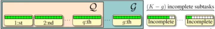
Fig. 1. Servers (yellow boxes) finish their respective subtasks in random order.
ofA. Therefore, the complexity scales with the product of the number of nonzero elements ofΨand the number of columns of A. Specifically,
σencode=|{(i, j) : Ψi,j6= 0}|n(σA+σM)−nσA.
Alternatively, we compute C by performing a decoding operation on A. In this case σencode is the decoding
com-plexity (see Section IV-B). Furthermore, since the decoding algorithms are designed to decode the entire codeword, each server has to compute all rows of C. Using this strategy the encoding delay is Dencode= K mNµ σencode K , K, K .
For each case we choose the strategy that minimizes the delay.
2) Map Phase: In the map phase, we compute in a dis-tributed fashion coded intermediate values, which will be later used to obtain vectors y1, . . . ,yN. Server S multiplies the
input vectors xj, j = 1, . . . , N, by all the coded rows of
matrixC it stores, i.e., it computes
Zj(S)={cxj : c∈ {BT : S∈ T }}, j= 1, . . . , N.
The map phase terminates when a set of servers G ⊆
{S1, . . . , SK} that collectively store enough values to decode
the output vectors have finished their map computations. We denote the cardinality of G by g. The (r, m) linear code proposed in [9] is an MDS code for which y1, . . . ,yN can
be obtained from any subset of q servers, i.e., g = q. We illustrate the completion of subtasks in Fig. 1.
We define the computational delay of the map phase as its average runtime per source row and vector y, i.e.,
Dmap= 1 mNµ σmap K , K, g ,
whereσmap =KηmN((n−1)σA+nσM), as all K servers
compute ηm inner products, each requiring n−1 additions andnmultiplications, for each of theN input vectors. In [9],
Dmap is referred to simply as the computational delay.
After the map phase, the computation of y1, . . . ,yN
pro-ceeds using only the servers inG. We denote byQ ⊆ Gthe set of the firstq servers to complete the map phase. Each of the
q servers in Q is responsible to computeN/q of the vectors
y1, . . . ,yN. Let WS be the set containing the indices of the
vectorsy1, . . . ,yN that serverS ∈ Qis responsible for. The
remaining servers in G assist the servers in Q in the shuffle phase.
3) Shuffle Phase: In the shuffle phase, intermediate values calculated in the map phase are exchanged between servers in
G until all servers in Q hold enough values to compute the vectors they are responsible for. As in [9], we allow creating and multicasting coded messages that are simultaneously use-ful for multiple servers. Furthermore, as in [8], we denote by
φ(j)the ratio between the communication load of unicasting the same message to each ofjrecipients and multicasting that message to j recipients. For example, if the communication load of multicasting a message to j recipients and unicasting a message to a single recipient is the same, we haveφ(j) =j. On the other hand, if the communication load of multicasting a message tojrecipients is equal to that of unicasting that same message to each recipient,φ(j) = 1. The total communication load of a multicast message is then given by φ(jj). The shuffle phase proceeds in three steps as follows.
1) Coded messages composed of several intermediate val-ues are multicasted among the servers inQ.
2) Intermediate values are unicasted among the servers in
Q.
3) Any intermediate values still missing from servers inQ are unicasted from the remaining servers inG, i.e., from the servers inG \ Q.
For a subset of servers S ⊂ QandS ∈ Q \ S, we denote the set of intermediate values needed by server S and known
exclusively by the servers inS byVS(S). More formally,
VS(S),{cxj: j∈ WS andc∈ {BT : T ∩ Q=S}}.
We transmit coded multicasts only between the servers in
Q, and each coded message is simultaneously sent to multiple servers. We denote by sq ,inf s: ηq X j=s αj≤1−η , αj , q−1 j K−q ηq−j q K K ηq , (1)
the smallest number of recipients of a coded message [9]. We remark thatmαj is the total number of coded values delivered
to each server via the coded multicast messages with exactlyj
recipients. More specifically, for eachj∈ {ηq, ηq−1, . . . , sq},
and every subset S ⊆ Q of size j + 1, the shuffle phase proceeds as follows.
1) For each S ∈ S, we evenly and arbitrarily split VS\(S)S intoj disjoint segments,VS\(S)S={VS\(S)S,S˜: ˜S∈ S \S}, and associate the segmentV(S)
S\S,S˜ to server S˜.
2) Server S˜∈ S multicasts the bit-wise modulo-2 sum of all the segments associated to it inS. More precisely, it multicasts⊕S∈S\S˜V
(S)
S\S,S˜ to the other servers inS \S˜,
where⊕denotes the modulo-2 sum operator.
By construction, exactly one value that each coded message is composed of is unknown to each recipient. The other values have been computed locally by the recipient. More precisely, for every pair of serversS,S˜∈ S, since serverShas computed locally the segments V(S
0)
S\S0,S˜ for all S0 ∈ S \ {S, S˜ }, it can cancel them from the message sent by server S˜, and recover the intended segment. We finish the shuffle phase by either unicasting any remaining needed values until all servers in
Q hold enough intermediate values to decode successfully, or by repeating the above two steps forj =sq−1. We refer to
these alternatives as shuffling strategy1and2, respectively. We always select the strategy achieving the lowest communication load. If any server in Q still needs more intermediate values
at this point, they are unicasted from other servers inG. This may happen only if a non-MDS code is used. We remark that it may be possible to opportunistically create additional coded multicasting opportunities by exploiting the remainingg−q
servers inG.
Definition 1. The communication load, denoted by L, is the number of unicasts and multicasts (weighted by their cost relative to a unicast) per source row and vectoryexchanged during the shuffle phase. Specifically, each unicasted message increases L by mN1 , and each message multicasted to j recipients increasesLby mN φj(j).
The communication load after completing the shuffle phase is given in [9]. If the shuffle phase finishes by unicasting the remaining needed values (strategy1), the communication load after completing the multicast phase is
ηq X
j=sq
αj φ(j).
If instead steps1)and2)are repeated forj=sq−1(strategy 2), the communication load is
ηq X
j=sq−1
αj φ(j).
For the scheme in [9], the total communication load is
LMDS= min ηq X j=sq αj φ(j)+ 1−η− ηq X j=sq αj, ηq X j=sq−1 αj φ(j) , (2) where 1−η−Pηq
j=sqαj is the communication load due to unicasting the remaining needed values.
4) Reduce Phase: Finally, in the reduce phase, the vectors
y1, . . . ,yN are computed. More specifically, server S ∈ Q
uses the locally computed sets Z1(S), . . . ,ZN(S) and the re-ceived messages to compute the vectors yj, ∀j ∈ WS. The
computational delay of the reduce phase is its average runtime per source row and output vectory, i.e.,
Dreduce= 1 mNµ σreduce q , q, q ,
where σreduce is the computational complexity (see
Sec-tion II-A) of the reduce phase.
Definition 2. The overall computational delay,D, is the sum of the encoding, map, and reduce phase delays, i.e., D = Dencode+Dmap+Dreduce.
C. Previously Proposed Coded Computing Schemes
Here we formally define the uncoded scheme (UC) and the coded computing schemes of [7]–[9] (which we refer to as the straggler coding (SC), coded MapReduce (CMR), and unified scheme, respectively) in terms of the model above. Specifically, to make a fair comparison with our coded computing scheme with parametersK,q,m, andη, we define the corresponding uncoded, CMR, SC, and unified schemes. When referring to the system parameters of a given scheme, we will write the scheme acronym in the subscript. We only
explicitly mention the parameters that differ. The number of servers K is unchanged for all schemes considered.
The uncoded scheme uses no erasure coding and no coded multicasting and has parameters ηUC = K1 and qUC = K,
implyingηUCqUC= 1. Furthermore, the encoding matrixΨUC
is them×midentity matrix and the coded matrix isCUC=A.
The CMR scheme [7] uses only coded multicasting, i.e.,
CCMR=AandqCMR=K. Furthermore, the fraction of rows
stored at each server is ηCMR = ηqK. We remark that there is
no reduce delay for this scheme, i.e., Dreduce= 0.
The SC scheme [8] uses an erasure code but no coded multicasting. For the corresponding SC scheme, the code rate is unchanged, i.e., qSC=q, and the fraction of rows stored at
each server isηSC= q1
SC. The encoding matrixΨSC of the SC
scheme is obtained by splitting the rows ofAintoqSCequally tall submatrices A1, . . . ,AqSC and applying a(K, qSC) MDS
code to the elements of each submatrix, thereby creating K
coded submatricesC1, . . . ,CK. The coded matrixCSC is the
concatenation ofC1, . . . ,CK, i.e., CSC= C1 .. . CK .
The unified scheme [9] uses both an erasure code and coded multicasting and has parameters ηunified = η and qunified =
q. Furthermore, the encoding matrix of the unified scheme,
Ψunified, is an (r, m)MDS code encoding matrix.
III. BLOCK-DIAGONALCODING
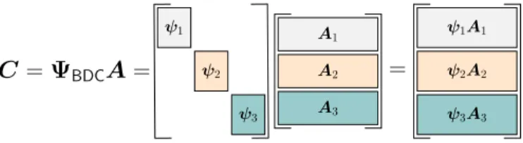
In this section, we introduce a BDC scheme for the problem of multiplying a matrix by a set of vectors. For large matrices, the encoding and decoding complexity of the proposed scheme is significantly lower than that of the scheme in [9], leading to a lower overall computational delay, as will be shown in Section VII. Specifically, the scheme is based on a block-diagonal encoding matrix of the form
ΨBDC= ψ1 . .. ψT ,
whereψ1, . . . ,ψT are Tr×mT encoding matrices of an(Tr,mT)
MDS code, for some integerT that dividesmandr. Note that the encoding given byΨBDCamounts to partitioning the rows
of A into T disjoint submatrices A1, . . . ,AT and encoding
each submatrix separately. We refer to an encodingΨBDCwith
T disjoint submatrices as aT-partitioned scheme, and to the submatrix of C = ΨBDCA corresponding to ψi as the i-th
partition. We remark that all submatrices can be encoded using the same encoding matrix, i.e., ψi=ψ,i= 1, . . . , T,
reduc-ing the storage requirements, and encodreduc-ing/decodreduc-ing can be performed in parallel if many servers are available. Notably, by keeping the ratio mT constant, the decoding complexity scales linearly with m. We further remark that the case ΨBDC=ψ
(i.e., the number of partitions is T = 1) corresponds to the scheme in [9], which we will sometimes refer to as the
unpartitioned scheme. We illustrate the BDC scheme with
T = 3 partitions in Fig. 2.
C
=
Ψ
BDCA
=
ψ2 ψ1 ψ3 A2 A3 A1=
ψ2A2 ψ1A1 ψ3A3Fig. 2. BDC scheme withT= 3partitions.
A. Assignment of Coded Rows to Batches
For a block-diagonal encoding matrixΨBDC, we denote by
c(it),t = 1, . . . , T andi= 1, . . . , r/T, thei-th coded row of
C within partitiont. For example,c(2)1 denotes the first coded row of the second partition. As described in Section II, the coded rows are divided into ηqKdisjoint batches. To formally describe the assignment of coded rows to batches we use a
K ηq
×T integer matrixP = [pi,j], wherepi,j is the number
of rows from partition j that are stored in batch i. In the sequel,P will be referred to as the assignment matrix. Note that, due to the MDS property, any set of m/T rows of a partition is sufficient to decode the partition. Thus, without loss of generality, we consider asequential assignment of rows of a partition into batches. More precisely, when first assigning a row of partitiontto a batch, we pickc(1t). Next time a row of partitiontis assigned to a batch we pickc(2t), and so on. In this manner, each coded row is assigned to a unique batch exactly once. The rows ofP are labeled by the subset of servers the corresponding batch is stored at, and the columns are labeled by their partition indices. For convenience, we refer to the pair
(ΨBDC,P) as the storage design. The assignment matrix P
must satisfy the following conditions.
1) The entries of each row ofP must sum up to the batch size, i.e., T X j=1 pi,j = r K ηq , 1≤i≤ K ηq .
2) The entries of each column of P must sum up to the number of rows per partition, i.e.,
(K ηq) X i=1 pi,j= r T, 1≤j≤T.
We clarify the assignment of coded rows to batches and the coded computing scheme in the following example.
Example 1 (m = 20, N = 4, K = 6, q = 4, η = 1/2,
T = 5). For these parameters, there arer/T = 6coded rows per partition, of whichm/T = 4are sufficient for decoding, and ηqK = 15 batches, each containing r/ ηqK
= 2 coded rows. We construct the storage design shown in Fig. 3 with
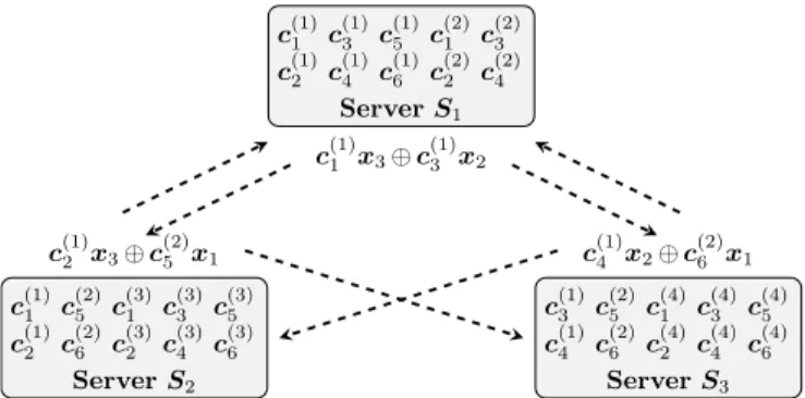
c(1)1 c (1) 3 c (1) 5 c (2) 1 c (2) 3 c(1)2 c (1) 4 c (1) 6 c (2) 2 c (2) 4 ServerS1 c(1)1 c (2) 5 c (3) 1 c (3) 3 c (3) 5 c(1)2 c (2) 6 c (3) 2 c (3) 4 c (3) 6 ServerS2 c(1)3 c (2) 5 c (4) 1 c (4) 3 c (4) 5 c(1)4 c (2) 6 c (4) 2 c (4) 4 c (4) 6 ServerS3 c(1)5 c (3) 1 c (4) 1 c (5) 1 c (5) 3 c(1)6 c (3) 2 c (4) 2 c (5) 2 c (5) 4 ServerS4 c(2)1 c (3) 3 c (4) 3 c (5) 1 c (5) 5 c(2)2 c (3) 4 c (4) 4 c (5) 2 c (5) 6 ServerS5 c(2)3 c (3) 5 c (4) 5 c (5) 3 c (5) 5 c(2)4 c (3) 6 c (4) 6 c (5) 4 c (5) 6 ServerS6
Fig. 3. Storage design form= 20,N = 4,K= 6,q= 4,η= 1/2, and T = 5. K ηq ×T = 15×5assignment matrix P = 1 2 3 4 5 (S1, S2) 2 0 0 0 0 (S1, S3) 2 0 0 0 0 (S1, S4) 2 0 0 0 0 (S1, S5) 0 2 0 0 0 .. . ... (S4, S6) 0 0 0 0 2 (S5, S6) 0 0 0 0 2 , (3)
where rows are labeled by the subset of servers the batch is stored at, and columns are labeled by the partition index. In this case rows c(1)1 and c
(1)
2 are assigned to batch 1, c (1) 3
and c(1)4 are assigned to batch2, and so on. For this storage
design, any g = 4 servers collectively store at least 4 coded rows from each partition. However, some servers store more rows than needed to decode some partitions, suggesting that this storage design is suboptimal.
Assume that G = {S1, S2, S3, S4} is the set of g = 4
servers that finish their map computations first. Also, assign vector yi to server Si, i= 1,2,3,4. We illustrate the coded shuffling scheme for S = {S1, S2, S3} in Fig. 4. Server
S1 multicasts c(1)1 x3⊕c(1)3 x2 to S2 and S3. Since S2 and
S3 can cancel c(1)1 x3 and c(1)3 x2, respectively, both servers
receive one needed intermediate value. Similarly,S2multicasts
c(1)2 x3⊕c(2)5 x1, while S3 multicasts c(1)4 x2⊕c(2)6 x1. This
process is repeated for S ={S2, S3, S4},S ={S1, S3, S4},
and S = {S1, S2, S4}. After the shuffle phase, we have sent 12 multicast messages and 30unicast messages, resulting in a communication load of (12 + 30)/20/4 = 0.525, a 50% increase from the load of the unpartitioned scheme (0.35, given by(2)). In this case,S1received additional intermediate
values from partition2, despite already storing enough, further indicating that the assignment in (3)is suboptimal.
IV. PERFORMANCE OF THEBLOCK-DIAGONALCODING In this section, we analyze the impact of partitioning on the performance. We also prove that we can partition up to the batch size, i.e., T = r/ K
ηq
, without increasing the communication load and the computational delay of the map phase with respect to the original scheme in [9].
A. Communication Load
For the unpartitioned scheme of [9], G = Q, and the number of remaining values that need to be unicasted after the multicast phase is constant regardless which subset Q
c(1)1 c (1) 3 c (1) 5 c (2) 1 c (2) 3 c(1)2 c (1) 4 c (1) 6 c (2) 2 c (2) 4 ServerS1 c(1)1 x3⊕c(1)3 x2 c(1)1 c (2) 5 c (3) 1 c (3) 3 c (3) 5 c(1)2 c (2) 6 c (3) 2 c (3) 4 c (3) 6 ServerS2 c(1)2 x3⊕c(2)5 x1 c(1)3 c (2) 5 c (4) 1 c (4) 3 c (4) 5 c(1)4 c (2) 6 c (4) 2 c (4) 4 c (4) 6 ServerS3 c(1)4 x2⊕c(2)6 x1
Fig. 4. Multicasting coded values between serversS1,S2, andS3.
of servers finish first their map computations. However, for the BDC (partitioned) scheme, both g and the number of remaining unicasts may vary.
For a given assignment matrix P and a specific Q, we denote by UQ(S)(P) the number of remaining values needed after the multicast phase by serverS∈ Q, and by
UQ(P),
X
S∈Q
UQ(S)(P) (4)
the total number of remaining values needed by the servers in
Q. Note that bothUQ(S)(P)andUQ(P)depend on the strategy used to finish the shuffle phase (see Section II-B3). We remark that all setsQ are equally likely. Let Qq denote the superset
of all setsQ. Furthermore, we denote byLQ(P)the average communication load of the messages that are unicasted after the multicasting step (see Section II-B3), i.e.,
LQ(P), 1 mN 1 |Qq| X Q∈Qq UQ(P). (5)
When needed we write L(1)Q (P) and L(2)Q (P), where the superscript denotes the strategy used to finish the shuffle phase. For a given storage design (ΨBDC,P), the communication
load of the BDC scheme is given by
LBDC(ΨBDC,P) = min ηq X j=sq αj φ(j)+L (1) Q (P), ηq X j=sq−1 αj φ(j)+L (2) Q (P) . (6)
Note that the load due to the multicast phase is independent of the level of partitioning. Furthermore, for the unpartitioned schemeL(2)Q = 0 by design.
We first explain how UQ(S) is evaluated. Let u(QS) be a vector of length T, where the t-th element is the number of intermediate values from partition t stored by server S
at the end of the multicast phase. Furthermore, each row of P corresponds to a batch, and coded multicasting is made possible by storing each batch at multiple servers. The intermediate values transmitted during the multicast phase thus correspond to rows of P. The vector u(QS) is then computed by adding some set of rows ofP. The indices of the rows to add depend onQ andS (see Section II-B3).
We denote by
u(QS)
tthe t-th element of the vectoru (S)
Q .
The number of valuesUQ(S) is given by adding the number of intermediate values still needed for each partition, i.e.,
UQ(S)= T X t=1 maxm T − u(QS) t,0 . (7) Its sum over all S ∈ Q gives UQ(P) (see (4)). Averaging UQ(P)over all Qand normalizing yieldsLQ(P)(see (5)). Example 2 (Computing u(QS)). We consider the same sys-tem as in Example 1. We again assume that G = Q =
{S1, S2, S3, S4}is the set ofg=q= 4servers that finish their
map computations first. During the multicast phase serverS1
receives the intermediate values in V(S1)
S\S1 for all sets S of cardinality j + 1 = 3 (see Section II-B3). In this case, we perform coded multicasting within the sets
• S ={S1, S2, S3},VS\(S1S)1 ={c5(2)x1,c(2)6 x1}, • S ={S1, S2, S4},V( S1) S\S1 ={c (3) 1 x1,c(3)2 x1}, • S ={S1, S3, S4},VS\(S1S)1 ={c (4) 1 x1,c(4)2 x1}. Note that V(S1)
{S2,S3} contains the intermediate values com-puted from the coded rows stored in the batch that labels the 6-th row of the assignment matrix P. In the same manner,
V(S1)
{S2,S4} and V
(S1)
{S3,S4} correspond to rows 7 and 10 of P, respectively. Furthermore, prior to the shuffle phase serverS1
stores the batches corresponding to rows 1 to5 of P. Thus,
u(S1)
{S1,S2,S3,S4} is equal to the sum of rows 1,2,3,4,5,6,7, and 10ofP. In this case,u(S1)
{S1,S2,S3,S4}= (6,6,2,2,0), and S1needs8more intermediate values, i.e.,U(
S1)
{S1,S2,S3,S4}= 8. Computing u(QS) for arbitrary Q and S then corresponds to summing the rows ofP corresponding to batches either stored by server S prior to the shuffle phase or received byS in the multicast phase. The row indices are computed as explained in Section II-B3.
For a givenΨBDC, the assignment of rows into batches can
be formulated as an optimization problem, where one would like to minimize LBDC(ΨBDC,P) over all assignments P.
More precisely, the optimization problem is
min
P∈PLBDC(ΨBDC,P),
wherePis the set of all assignmentsP. This is a computation-ally complex problem, since both the complexity of evaluating the performance of a given assignment and the number of assignments scale exponentially in the problem size (there are q Kq
vectors u(QS)). We address the optimization of the assignment matrix P in Section V.
B. Computational Delay
We consider the delay incurred by the encoding, map, and reduce phases (see Definition 2). As in [9], we do not consider the delay incurred by the shuffle phase as the computations it requires are simple in comparison. Note that in [9] only
Dmapis considered, i.e.,D=Dmap. However, one should not
neglect the computational delay incurred by the encoding and
reduce phases. Thus, we consider the overall computational delay
D=Dencode+Dmap+Dreduce.
The encoding delay Dencode is a function of the number of
nonzero elements ofΨBDC. As there are at most mT nonzero
elements in each row of a block-diagonal encoding matrix, for an encoding scheme withT partitions we have
σencode,BDC≤ m TrnσM+ m T −1 rnσA. (8)
The reduce phase consists of decoding theNoutput vectors and hence the delay it incurs depends on the underlying code and decoding algorithm. We assume that each partition is encoded using a Reed-Solomon (RS) code and is decoded using either the Berlekamp-Massey (BM) algorithm or the FFT-based algorithm proposed in [23], whichever yields the lowest complexity. To the best of our knowledge the algorithm proposed in [23] is the lowest complexity algorithm for decod-ing long RS codes. We measure the decoddecod-ing complexity by its associated shifted-exponential parameterσ(see Section II-A). The number of field additions and multiplications required to decode an (r/T, m/T) RS code using the BM algorithm is (r/T) (ξ(r/T)−1) and(r/T)2ξ, respectively, where ξ is the fraction of erased symbols [24]. Withξupper bounded by
1− q
K (the map phase terminates when a fraction of at least q
K symbols from each partition is available), the complexity
of decoding theT partitions for all N output vectors is upper bounded as σBM reduce,BDC≤N σA r2(1 − q K) T −r +σM r2(1 − q K) T . (9) On the other hand, the FFT-based algorithm has complexity
O(rlogr)[23]. We estimate the number of additions and mul-tiplications required for a given code lengthrby fitting a curve of the form a+brlog2(cr), where (a, b, c) are coefficients, to empiric results derived from the authors’ implementation of the algorithm. For additions the resulting parameters are
(2,8.5,0.867) and for multiplications they are (2,1,4). The resulting curves diverge negligibly at the measured points. The total decoding complexity for the FFT-based algorithm is
σFFT reduce,BDC=N T σA 2 + 8.5r T log2(0.867r/T) +N T σM 2 + r T log2(4r/T) . (10)
The encoding and decoding complexity of the unified scheme in [9] is given by evaluating (8) and either (9) or (10) (whichever gives the lowest complexity), respectively, for
T = 1. For the BDC scheme, by choosingTclose torwe can thus significantly lower the delay of the encoding and reduce phases. On the other hand, the scheme in [8] uses codes of length proportional to the number of serversK. The encoding and decoding complexity of the SC scheme in [8] is thus given by evaluating (8) and either (9) or (10) forT =m
q. C. Lossless Partitioning
Theorem 1. For T ≤ r/ ηqK
, there exists an assignment matrix P such that the communication load and the
com-putational delay of the map phase are equal to those of the unpartitioned scheme.
Proof:The computational delay of the map phase is equal to that of the unpartitioned scheme if any q servers hold enough coded rows to decode all partitions. For T =r/ K
ηq
we let P be a ηqK
×T all-ones matrix and show that it has this property by repeating the argument from [9, Sec. IV.B] for each partition. In this case, any set ofqservers collectively store ηqmT rows from each partition, and since each coded row is stored by at mostηqservers, anyqservers collectively store at least ηqmηqT = m
T unique coded rows from each partition.
The computational delay of the map phase is thus unchanged from the unpartitioned scheme. The communication load is unchanged ifUQ(S)is equal to that of the unpartitioned scheme for all Q and S. The number of values needed UQ(S) is computed from u(QS) (see (7)), which is the sum of l rows of P, for some integerl. For the all-ones assignment matrix, because all rows of P are identical, we have
UQ(S)=Tmaxm T −l,0
= max (m−T l,0),
which is the number of remaining values for the unpartitioned scheme.
Next, we consider the case where T < r/ ηqK . First, consider the case T = r/ ηqK
− j, for some integer j,
0 ≤ j < r
2(ηqK). We first set all entries of P equal to 1. At this point, the total number of unique rows ofC per partition stored by any set ofq servers is at least
m r/ K ηq = m r/ K ηq −j r/ K ηq −j r/ K ηq = m T r/ K ηq −j r/ K ηq . (11)
The number of coded rows per partition that are not yet as-signed is given byr/T multiplied by the fraction of partitions removed j r/(ηqK), i.e., 1 T rj r/ Kηq = 1 T mK qj r/ ηqK. (12) We assign these rows to batches such that an equal number of coded rows is assigned to each of theK servers, which is always possible due to the limitations imposed by the system model. Any set of q servers will thus store a fraction q/K
of these rows. The total number of unique coded rows per partition stored among any set of q servers is then lower bounded by the sum of (12) weighted by q/K and (11), i.e.,
m T r/ K ηq −j r/ ηqK + K qj r/ ηqK q K ! =m T,
showing that it is possible to decode all partitions using the coded rows stored over any set ofq servers.
The communication load is unchanged with respect to the case where the number of partitions isr/ ηqK
if and only if no server receives rows it does not need in the multicast phase. Due to decreasing the number of partitions from r/ ηqK
to
T =r/ K ηq
−j, we increase the number of coded rows needed to decode each partition by
m T − m r/ ηqK = 1 T mj r/ ηqK. (13) Furthermore, reducing the number of partitions increases the number of coded rows per partition stored among any set of
qservers (see (12) and the following text) by
1 T
mj
r/ Kηq. (14) Note that the number of additional rows needed to decode each partition (see (13)) is greater than or equal to the number of additional rows stored among the q servers (see (14)). It is thus impossible that too many coded rows are delivered for any partition.
Second, we consider the case T = r/( K ηq)−j
i , where j is
chosen as for the first case above and where i is a positive integer. Now, we first set all elements ofP toi. At this point the number of unique rows ofCper partition stored by any set ofqservers is given by (11) multiplied by a factori(since we set each element of P toi instead of one). Furthermore, the number of coded rows per partition that are not yet assigned is given by (12). Therefore, by using the same strategy as for i = 1 and assigning the remaining rows to batches such that an equal number of rows is assigned to each of the K
servers, we are guaranteed that the communication load and the computational delay are unchanged also in this case.
V. ASSIGNMENTSOLVERS
ForT ≤r/ ηqK
partitions, we can choose the assignment matrix P as described in the proof of Theorem 1. For the case where T > r/ ηqK
, we propose two solvers for the problem of assigning rows into batches: a heuristic solver that is fast even for large problem instances, and a hybrid solver combining the heuristic solver with a branch-and-bound solver. The branch-and-bound solver produces an optimal assignment but is significantly slower, hence it can be used as stand-alone only for small problem instances. We use a dynamic programming approach to speed up the branch-and-bound solver by cachingu(QS) for allS andQ ∈Qq. We index each
cached u(QS) by the batches it is computed from. Whenever
UQ(S)drops to0due to assigning a row to a batch, we remove the correspondingu(QS)from the index. We also store a vector of length T with the i-th entry giving the number of vectors
u(QS) that miss intermediate values from the i-th partition. Specifically, the i-th element of this vector is the number of vectorsu(QS) for which the i-th element is less than mT. This allows us to efficiently assess the impact on LQ(P) due to
assigning a row to some batch. Sinceu(QS)is of lengthT and because the cardinality ofQandQqisqand Kq
, respectively, the memory required to keep this index scales asOT q Kq and is thus only an option for small problem instances.
For all solvers, we first label the batches lexiographically and then optimizeLBDC in (6). For example, forηq= 2, we
Algorithm 1: Heuristic Assignment Input : P,d,K,T, andηq for0≤a < d K ηq do i← ba/dc+ 1 j ←(amodT) + 1 pi,j←pi,j+ 1 end return P
on. The solvers are available under the Apache 2.0 license [25]. We remark that choosingP is similar to the problem of designing the coded matrices stored by each server in [12].
A. Heuristic Solver
The heuristic solver is inspired by the assignment matrices created by the branch-and-bound solver for small instances. It creates an assignment matrixP in two steps. We first set each entry of P to Y , $ r K ηq ·T % ,
thus assigning the first ηqK
Y rows of each partition to batches such that each batch is assigned Y T rows. Letd=r/ ηqK
−
Y T be the number of rows that still need to be assigned to each batch. Ther/T− ηqK
Y rows per partition not assigned yet are assigned in the second step as shown in Algorithm 1.
Interestingly, for T≤r/ ηqK
the heuristic solver creates an assignment matrix satisfying the requirements outlined in the proof of Theorem 1. In the special case of T =r/ K
ηq
, the all-ones matrix is produced.
B. Branch-and-Bound Solver
The branch-and-bound solver finds an optimal solution by recursively branching at each batch for which there is more than one possible assignment and considering all options. The solver is initially given an empty assignment matrix, i.e., an all-zeros ηqK×T matrix. For each branch, we lower bound the value of the objective function of any assignment in that branch and only investigate branches with possibly better assignments. The branch-and-bound operations given below are repeated until there are no more potentially better solutions to consider.
1) Branch: For the first row ofP with remaining assign-ments, branch on every available assignment for that row. More precisely, find the smallest index i of a row of the assignment matrixP whose entries do not sum up to the batch size, i.e., T X j=1 pi,j< r K ηq .
For row i, branch on incrementing the element pi,j by1 for
all columns (with index j) such that their entries do not sum up to the number of coded rows per partition, i.e.,
(K ηq) X i=1 pi,j< r T.
2) Bound: We use a dynamic programming approach to lower boundLBDC for a subtree. Specifically, for each rowi
and columnj ofP, we store the number of vectorsu(QS)that are indexed by rowiand where thej-th element satisfies
m T − u(QS) j >0.
Assigning a coded row to a batch can at most reduceLBDC
by 1/(mN|Qq|) for each u(QS) indexed by that batch. We compute the bound by assuming that nou(QS)will be removed from the index for any subsequent assignment.
C. Hybrid Solver
The branch-and-bound solver can only be used by itself for small instances. However, it can be used to complete a
partialassignment matrix, i.e., a matrix P for which not all rows have entries that sum up to the batch size. The branch-and-bound solver then completes the assignment optimally. We first find a candidate solution using the heuristic solver and then iteratively improve it using the branch-and-bound solver. In particular, we decrement by1a random set of entries of P and then use the branch-and-bound solver to reassign the corresponding rows optimally. We repeat this process until the average improvement between iterations drops below some threshold.
VI. LUBYTRANSFORMCODES
In this section, we consider LT codes [16] for use in distributed computing. Specifically, we consider a distributed computing system where Ψ is an LT code encoding matrix, denoted by ΨLT, of fixed rate mr. As explained in Section II,
we divide ther coded rows ofC =ΨLTAinto ηqK
disjoint batches, each of which is stored at a unique subset of sizeηq
of the K servers. For this scheme, due to the random nature of LT codes, we can assign coded rows to batches randomly. The distributed computation is carried out as explained in Section II-B, i.e., we wait for the fastest g ≥ q servers to complete their respective computations in the map phase, perform coded multicasting during the shuffle phase, and carry out the decoding of theN output vectors in the reduce phase. Let Ω denote the degree distribution and Ω(d) the proba-bility of degree d. Also, let Ω¯ be the average degree. Then, each row of the encoding matrix ΨLT is constructed in the
following manner. Uniformly at random selectdunique entries of the row, wheredis drawn from the distributionΩ. For each of these d entries, assign to it a nonzero element selected uniformly at random from F2l. Specifically, we consider the case where Ωis the robust Soliton distribution parameterized byM andδ, whereM is the location of the spike of the robust component andδis a parameter for tuning the decoding failure probability for a givenM [16].
A. Inactivation Decoding
We assume that decoding is performed using inactivation decoding [17]. Inactivation decoding is an efficient maximum likelihood decoding algorithm that combines iterative decod-ing with optimal decoddecod-ing in a two-step fashion and is widely
used in practice. As suggested in [17], we assume that the optimal decoding phase is performed by Gaussian elimination. In particular, iterative decoding is used until the ripple is empty, i.e., until there are no coded symbols of degree 1, at which point an input symbol is inactivated. The iterative decoder is then restarted to produce a solution in terms of the inactivated symbol. This procedure is repeated until all input symbols are either decoded or inactivated. Note that the value of some input symbols may be expressed in terms of the values of the inactivated symbols at this point. Finally, optimal decoding of the inactivated symbols is performed via Gaussian elimination, and the decoded values are back-substituted into the decoded input symbols that depend on them. The decoding schedule has a large performance impact. Our implementation follows the recommendations in [17]. It is important to tune the parametersM andδto minimize the number of inactivations. Due to the nature of LT codes, we need to collectm(1 +)
intermediate values for each vector y before decoding. We refer to as the overhead. Under inactivation decoding, and for a given overhead, the probability of decoding failure with an overhead of at most, denoted byPf(), is lower bounded
by [26] Pf()≥ m X i=1 (−1)i+1 m i m X d=1 Ω(d) m−i d m d !m(1+) . (15) Note thatPf()is the CDF for the random variable “decoding
is not possible at a given overhead .” Furthermore, the lower bound (15) well approximates the failure probability for an overhead slightly larger than = 0. Denote by FDS() the
probability of decoding being possible at an overhead of at most . It follows that
FDS() = 1−Pf().
We find the decoding success probability density function (PDF) by numerically differentiatingFDS().
B. Code Design
We design LT codes for a minimum overheadmin, i.e., we
collect at least m(1 +min) coded symbols from the servers
before attempting to decode, and a target failure probability
Pf,target = Pf(min). We remark that increasing min and
Pf,target leads to a lower average degree Ω¯, and thus to less
complex encoding and decoding and subsequently to a lower computational delay for encoding and decoding. The tradeoff is that the communication load increases as more intermediate values need to be transferred over the network on average. Furthermore, increasing min and Pf,target may increase the
average number of serversgrequired to decode. We thus need to balance the computational delay of the encoding and reduce phases against that of the map phase to achieve a low overall computational delay. Furthermore, waiting for more thang=q
servers typically increases the overall computational delay by more than what is saved by the less complex encoding and decoding given by the larger min andPf,target. We thus
choose min and Pf,target such that decoding is possible with
high probability using the number of coded rows stored at
any set of q servers. Note that the overhead required for decoding may be larger thanmin. We take this into account by
numerically integrating the decoding success PDF multiplied by the performance of the scheme as a function of the overhead
.
For a givenminandPf,target, we find a pair(M, δ)that
min-imizes the decoding complexity (see Section VI-C) under the constraint that Pf(min)≈ Pf,target. Essentially, we minimize
the computational delay of the reduce phase for a fixed delay of the map phase. We remark that LT codes with low decoding complexity have a low average degree Ω¯, and thus also low encoding complexity. Note that for a given M, decreasingδ
lowers the failure probability, but also increases the decoding complexity. We find good pairs (M, δ) by selecting through binary search the largestM such that there exists aδfor which the lower bound onPf(min)in (15) is approximately equal to
Pf,target. This heuristic produces codes with complexity very
close to those found using basin-hopping [27] combined with the Powell optimization method [28].
C. Computational Delay
There are on averageΩ¯ nonzero entries in each row of the LT code encoding matrix. The LT code encoding complexity is thus given by
σencode,LT= ¯ΩrnσM+ ( ¯Ω−1)rnσA.
We simulate the complexity of the decoding σreduce,LT.
Fur-thermore, we assume that the decoding complexity depends only on min, i.e., we evaluate the decoding complexity only
at=min, and simulate the number of serversg required for
a given overhead.
D. Communication Load
The coded multicasting scheme (see Section II-B3) is de-signed for the case where we needmintermediate values per vectory. Here, we tune it for the case where we instead need at least m(1 + min) intermediate values by increasing the
number of coded multicast messages sent. Note that the coded multicasting scheme is greedy in the sense that it starts by multicasting coded messages to the largest possible number of recipients and then gradually lowers the number of recipients. Specifically, we perform the shuffle phase with (see (1))
sq,LT,inf s: ηq X j=s αj≤(1 +min)−η .
The communication load of the LT code-based scheme for a given≥min is then given by
LLT= min ηq X j=sq,LT αj φ(j)+ (1 +)−η− ηq X j=sq,LT αj , ηq X j=sq,LT−1 αj φ(j)+ max (1 +)−η− ηq X j=sq,LT−1 αj,0 .
0.5 0.6 0.7 0.8 0.9 1 1.1 L 101 102 103 0.5 1 1.5 2 2.5 3 3.5 4 T D BDC, Heuristic LT LT, Partitioned CMR SC Unified
Fig. 5. The tradeoff between partitioning and performance for m= 6000, n= 6000,K= 9,q= 6,N= 6000, andη= 1/3.
E. Partitioning of the LT Code-Based Scheme
We can apply partitioning to the LT code-based scheme in the same manner as for the BDC scheme. Specifically, we consider a block-diagonal encoding matrix ΨBDC−LT, where
the blocks ψ1, . . . ,ψT are LT code encoding matrices. In
particular, we consider the case where the number of parti-tions T is equal to the partitioning limit of Theorem 1, i.e.,
T = r/ ηqK
. In this case the all-ones assignment matrix P
introduced in the proof of Theorem 1 is a valid matrix. By using this assignment matrix and identical encoding matrices for each of the partitions, i.e., ψi = ψ, i = 1, . . . , T,
the encoding and decoding complexity of each partition is identical regardless of which set of servers G first completes the map phase. Furthermore, by the same argument as in the proof of Theorem 1, we are guaranteed that if any partition can be decoded using the coded rows stored at the set of servers
G, all other partitions can also be decoded.
VII. NUMERICALRESULTS
We present numerical results for the proposed BDC and LT code-based schemes and compare them with the schemes in [7]–[9]. Furthermore, we compare the performance of the BDC scheme with assignment P produced by the heuristic and hybrid solvers. We also evaluate the performance of the LT code-based scheme for differentPf,target andmin. For each
plot, the field size is equal to one more than the largest number of coded rows considered for that plot, r+ 1, rounded up to the closest power of2. The results, except those in Fig. 12, are normalized by the performance of the uncoded scheme. Unless stated otherwise, the assignment P is given by the heuristic solver. As in [9], we assume thatφ(j) =j.
0.4 0.5 0.6 0.7 0.8 0.9 1 1.1
L BDC, HeuristicCMR LTSC LT, PartitionedUnified
101 102 0.5 1 1.5 2 2.5 K D
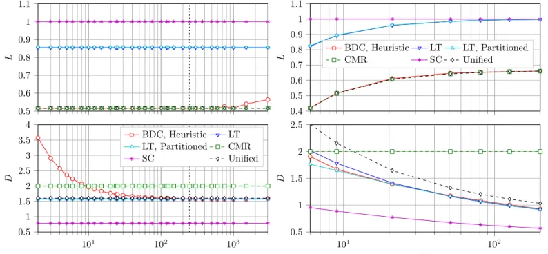
Fig. 6. Performance dependence on system size forηq= 2,n=m/100, ηm= 2000, code ratem/r= 2/3, andN= 500qvectors.
A. Coded Computing Comparison
In Fig. 5, we depict the communication load L (see Def-inition 1) and the computational delay D (see Definition 2) as a function of the number of partitions, T. The system parameters are m = 6000, n = 6000, K = 9, q = 6,
N = 6000, and η = 1/3. The parameters of the CMR and SC schemes are qCMR = 9, ηCMR = 29, and ηSC = 16.
The minimum overhead for the LT code-based scheme is
min = 0.3 and its target failure probability isPf,target = 0.1.
For up to r/ Kηq
= 250 partitions (marked by the vertical dotted line), the BDC scheme does not incur any loss inDmap
and communication load with respect to the unified scheme (see Theorem 1). Furthermore, the BDC scheme yields about a
2% lower delay compared to the unified scheme forT = 1000. The delay of the LT code-based scheme is slightly worse than that of the BDC scheme, and the load is about65%higher (for
T = 250). Partitioning the LT code-based scheme increases the communication load and reduces the computational delay by about0.5%. We remark that the number of partitions for the LT code-based scheme is fixed at r/ K
ηq
. For heavy partitioning of the BDC scheme, a tradeoff between partitioning level, communication load, and map phase delay is observed. For example, with3000partitions (the maximum possible), there is about a10%increase in communication load over the unified scheme. Note that the gain in computational delay saturates, thus there is no reason to partition beyond a given level. The load of the SC scheme is about twice that of our proposed schemes and the delay is about half. Finally, the delay of the BDC and the LT code-based scheme is about25% lower compared to the CMR scheme for T >100.
In Fig. 6, we plot the performance for a constantηq = 2,
n = m/100, ηm = 2000, code rate m/r = 2/3, and
N = 500qvectors as a function of the number of servers,K. The ratiom/nis motivated by machine learning applications,
0.4 0.5 0.6 0.7 0.8 0.9 1 L BDC, Heuristic LT LT, Partitioned Unified 101 102 0 5 10 15 20 25 K D
Fig. 7. Performance dependence on system size with constant complexity of the map phase per server,m/r= 2/3,ηq= 2,n=m/100, andN=n. where the number of rows and columns often represent the number of samples and features, respectively. Note that the number of arithmetic operations performed by each server in the map phase increases with K. We choose the number of partitions T that minimizes the delay under the constraint that the communication load is at most 1% higher compared to the unified scheme. The parameters of the LT code-based scheme aremin= 0.335andPf,target= 0.1. The results shown
are averages over 1000randomly generated realizations ofG. Our proposed BDC scheme outperforms the unified scheme in terms of computational delay by between about 25% (for
K = 6) and 10% (for K = 201). Furthermore, the delay of both the BDC and LT code-based schemes are about 50% lower than that of the CMR scheme forK= 201. ForK= 6
the computational delay of the unpartitioned and partitioned LT code-based schemes is about 5% higher and 8% lower compared to the BDC scheme, respectively. For K= 201the delay of the LT code-based scheme is about 1% lower than that of the BDC scheme. However, the communication load is about 45% higher. Finally, the communication load of the BDC scheme is between about 42% (for K = 6) and 66%
(for K= 201) of that of the SC scheme.
In Fig. 7, we show the performance for code rate m/r = 2/3, ηq = 2, and a fixed workload per server as a func-tion of K. Specifically, we fix the number of additions and multiplications computed by each server in the map phase to 108 (
±5% to find valid parameters) and scale m, n, N
with K. The number of rowsm of A takes values between
12600 and59800, and we letn =m/100 and N =n. The number of partitions T is selected in the same way as for Fig. 6. The results shown are averages over 1000 randomly generated realizations of G. The computational delay of the unified scheme is about a factor 20 higher than that of the BDC scheme for K = 300. The computational delay of the partitioned LT code-based scheme is similar to that of the BDC
0.5 0.6 0.7 0.8 0.9 1 L BDC, Heuristic LT (0.3,10−1) LT (0.3,10−3) LT (0.37,10−1) LT (0.37,10−3) 103 104 2 2.05 2.1 2.15 2.2 2.25 2.3 n D
Fig. 8. Performance dependence on the number of columns nof A for m= 2400,K= 9,q= 6,N= 60,T= 240, andη= 1/3. The parameters of the LT code-based scheme are given in the legend as(min, Pf,target). scheme, while the delay of the unpartitioned LT code-based scheme is about60% higher. Furthermore, the communication load of the LT code-based scheme is about 45% higher compared to those of the unified and BDC schemes.
In Fig. 8, we plot the performance of the BDC and LT code-based schemes as a function of the number of columns
n. The system parameters are m = 2400, K = 9, q = 6,
N = 60,T = 240, andη= 1/3. The communication load of the LT code-based scheme depends primarily on the minimum overhead min and the computational delay primarily on the
target failure probability Pf,target. We remark that a higher
Pf,target allows for using codes with lower average degree and
thus less complex encoding and decoding. For n = 20000, the computational delay of the LT code-based scheme with
Pf,target = 0.1 is about 1.5% lower than that of the BDC
scheme. For Pf,target = 0.001, the computational delay is
about3% and1.5% higher than that of the BDC scheme when
min = 0.3 and min = 0.37, respectively. On the other hand,
the communication load of the LT code-based scheme with
min = 0.3 and min = 0.37 is about 41% and 44% higher
than that of the BDC scheme, respectively.
B. Assignment Solver Comparison
In Figs. 9 and 10, we plot the performance of the BDC scheme with assignment P given by the heuristic and the hybrid solver. We also give the average performance over
100 random assignments. The vertical dotted line marks the partitioning limit of Theorem 1. The parameters in Figs. 9 and 10 are identical to those in Figs. 5 and 6, respectively.
In Fig. 9, we plot the performance as a function of the number of partitions, T. For T less than about 200, the performance for all solvers is identical. On the other hand, for
T >200both the computational delay and the communication load are reduced with P from the heuristic solver over the
0.5 0.52 0.54 0.56 0.58 0.6 L BDC, Heuristic BDC, Hybrid BDC, Random 101 102 103 1.5 2 2.5 3 3.5 4 T D
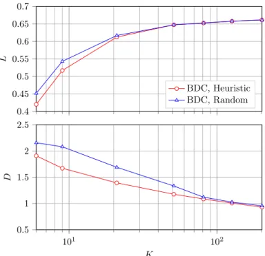
Fig. 9. Solver performance as a function of partitioning form = 6000, n= 6000,K= 9,q= 6,N= 6000, andη= 1/3. 0.4 0.45 0.5 0.55 0.6 0.65 0.7 L BDC, Heuristic BDC, Random 101 102 0.5 1 1.5 2 2.5 K D
Fig. 10. Solver performance as a function of system size forηq= 2,n=
m/100,ηm= 2000, code ratem/r= 2/3, andN= 500qvectors. random assignments (about 5% for load and 47% for delay atT = 3000). A further improvement in communication load can be achieved using the hybrid solver, but at the expense of a possibly larger computational delay.
In Fig. 10, we plot the performance as a function of the number of servers, K. The results shown are averages over
1000 randomly generated realizations of G. For K = 6, the communication load of the heuristic solver is about5%lower than that of the random assignments, but for K = 201 the difference is negligible. In terms of computational delay, the
2 2.5 3 3.5 4 4.5 5 5.5 0.1 0.2 0.3 0.4 0.5 0.6 0.7 0.8 0.9 D L BDC, Heuristic, 1% BDC, Heuristic, 10% LT, Partitioned Unified
Fig. 11. The tradeoff between communication load and computational delay forK= 14,m= 50000±3%,n= 500,N= 840, andη= 1/2. heuristic solver outperforms the random assignments by about
18% and 3% for K = 9 and K = 201, respectively. The hybrid solver is too computationally complex for use with the largest systems considered.
C. Tradeoff Between Communication Load and Computa-tional Delay
In Fig. 11, we show the tradeoff between communication load and computational delay. The parameters are K = 14,
m = 50000 (±3% to find valid parameters), n = 500,
N = 840, andη= 1/2. Note that the code rate is decreasing toward the bottom of the plot. We select the number of partitions T that minimizes the delay while the load is at most 1% or 10% higher compared to the unified scheme. Allowing a 10% increased load gives up to about 7% lower delay compared to allowing a 1% increase. For the topmost data point of the BDC and unified schemes the encoding complexity dominates, and there is no reason to operate at this point since both the delay and load can be reduced. The parameters of the partitioned LT code-based scheme are
min = 0.3 and Pf,target = 10−1. For the data point with
minimum computational delay, the LT code-based scheme yields about 15% lower delay at the expense of about a
30% higher load compared to the BDC scheme. Finally, the computational delay of the BDC scheme is between about47% and4% lower compared to the unified scheme for the topmost and bottommost data points, respectively.
D. Computational Delay Deadlines
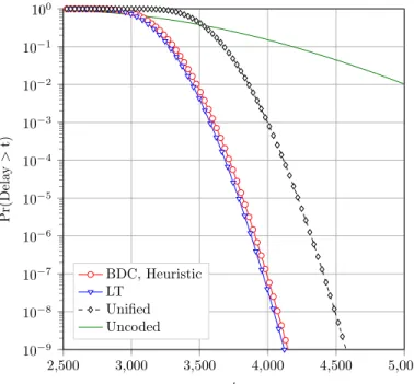
In Fig. 12, we plot the probability of a computation not finishing before a deadline t, i.e., the probability of the computational delay being larger than t. As in [29], we plot the complement of the CDF of the delay in logarithmic scale.
2,500 3,000 3,500 4,000 4,500 5,000 10−9 10−8 10−7 10−6 10−5 10−4 10−3 10−2 10−1 100 t P r( D el ay > t) BDC, Heuristic LT Unified Uncoded
Fig. 12. The probability of a computation not finishing before a deadlinet forK= 201,q= 134,m= 134000,n= 1340,N= 67000vectors,T = 6700partitions, code ratem/r= 2/3,min= 0.335, andPf,target= 10−9. On the horizontal axis, we show the deadline t. The system parameters are K= 201,q= 134, m= 134000, n= 1340,
N = 67000 vectors, T = 6700 partitions, and code rate
m/r = 2/3. The parameters for the LT code-based scheme are min = 0.335 and Pf,target = 10−9. The results are due
to simulations. In particular, we simulate the decoding failure probability of LT codes for various t and extrapolate from these points under the assumption that the decoding failure probability is Gamma distributed. The fitted values deviate negligibly from the simulated values.
When the deadline ist= 3500, the probability of exceeding the deadline is about0.4for the unified and uncoded schemes. For the BDC scheme the probability is only about 7·10−3. The probability is slightly lower for the LT code-based scheme, about 4·10−3. If we instead consider a deadline t = 4000, the probability of exceeding the deadline is about 10−3 and 0.15 for the unified and uncoded schemes, respectively. For the BDC scheme the probability of exceeding the deadline is about 9·10−8, i.e., 4 orders of magnitude lower compared to the unified scheme. The LT code-based scheme further improves the performance with a probability of exceeding the deadline of about3·10−8. We remark that for the data point with minimum delay in Fig. 11, the LT code-based scheme has a significant advantage over the BDC scheme in terms of meeting a short deadline.
E. Alternative Runtime Distribution
Here, we consider a runtime distribution with CDF
FH(h;σ) = (
1−e−(h−σ)/β, forh
≥σ
0, otherwise ,
where σ is the shift and β is a parameter that scales the tail of the distribution, i.e., it differs from the one considered previously by that the scale of the tail may be different from
101 102 20 21 22 23 24 25 K D BDC, Heuristic,ω= 0 Unified,ω= 0 BDC, Heuristic,ω= 1 Unified,ω= 1 BDC, Heuristic,ω= 10 Unified,ω= 10 BDC, Heuristic,ω= 100 Unified,ω= 100
Fig. 13. Computational delay as a function of system size for varying scale of the tail of the runtime distribution. The system parameters and communication load are identical to those in Fig. 7.
the shift. It is equal to the previously considered distribution if β = σ. This model has been used to model distributed computing in, e.g., [30]. Under this model we assume that the reduce delay of the uncoded scheme follows the distribution above with parameters β and σUC,reduce = 0 since each
server has to assemble the final output from the intermediate results regardless coding is used or not. We assume that the encoding delay of the uncoded scheme is zero. Denote byσc
the computational complexity of matrix-vector multiplication for the BDC and unified schemes. We let β = ωσc for
ω= 0,1,10,100. In Fig. 13, we plot the computational delay normalized by that of the uncoded scheme. The system pa-rameters (and thus also the communication load) are identical to those in Fig. 7.
We observe the greatest gain of the BDC scheme over the unified scheme for small ω since the benefits of straggler coding are small compared to the added delay due to encoding and decoding, which is significant for the unified scheme. For largerω the benefits of straggler coding are larger while the delay due to encoding and decoding remains constant. Hence, the performance of both schemes converge. However, even for
ω= 100the delay of the unified scheme is about33% higher than that of the BDC scheme for the largest system considered (K= 300). We remark that for the example considered in [30] the parametersβ =σ= 1, i.e.,ω= 1, are used.
VIII. CONCLUSION
We introduced two coding schemes for distributed matrix multiplication. One is based on partitioning the matrix into submatrices and encoding each submatrix separately using MDS codes. The other is based on LT codes. Compared to the earlier scheme in [9] and to the CMR scheme in [7], both proposed schemes yield a significantly lower overall compu-tational delay. For instance, for a matrix of size59800×598,