Service workload patterns for QoS-driven cloud resource management

RESEARCH

Service Workload Patterns for QoS-driven Cloud

Resource Management

Li Zhang

, Yichuan Zhang

, Pooyan Jamshidi

, Lei Xu

and Claus Pahl

Abstract

Cloud service providers negotiate SLAs for

customer services they offer based on the reliability of performance and availability of their lower-level platform infrastructure. While availability

management is more mature, performance management is less reliable. In order to support a continuous approach that supports the initial static infrastructure configuration as well as dynamic reconfiguration and auto-scaling, an accurate and efficient solution is required. We propose a prediction technique that combines a workload pattern mining approach with a traditional

collaborative filtering solution to meet the accuracy and efficiency requirements. Service workload patterns abstract common infrastructure workloads from monitoring logs and act as a part of a first-stage high-performant configuration mechanism before more complex traditional methods are considered. This enhances current reactive rule-based scalability approaches and basic prediction techniques by a hybrid prediction solution. Uncertainty and noise are additional challenges that emerge in multi-layered, often federated cloud architectures. We specifically add log smoothing combined with a fuzzy logic approach to make the prediction solution more robust in the context of these challenges.

Keywords: Quality of Service; Resource Management; Cloud Scalability; Web and Cloud Services; QoS Prediction; Workload Pattern Mining; Uncertainty

1 INTRODUCTION

Quality of Service (QoS) is the basis of cloud service and resource configuration management [1] [2]. Cloud

*_{Correspondence: [email protected]}

2_{IC4 / School of Computing, Dublin City University, Dublin, Ireland}

Full list of author information is available at the end of the article

service providers – whether at infrastructure, platform or software level – provide quality guarantees usually in terms of availability and performance to their cus-tomers in the form of service-level agreements (SLAs) [3]. Internally, the respective service configuration in terms of available resources then needs to make sure that the SLA obligations are met [4]. To facilitate SLA conformance, virtual machines (VMs) can be config-ured and scaled up/down in terms of CPU cores and memory, deployed with storage and network capabili-ties. Some current cloud infrastructure solutions allow users to define rules manually to scale up or down to maintain performance levels.

QoS factors like service performance in terms of re-sponse time or availability may vary depending on net-work, service execution environment and user require-ments, making it hard for providers to choose an ini-tial configuration and scale this up/down to maintain the SLA guarantees, but also optimising resource util-isation at the same time. We utilise QoS prediction techniques here, but rather than bottom-up predict-ing QoS from monitored infrastructure metrics [5] [6] [7], we reverse the idea, resulting in a novel technique for pattern-based resource configuration.

A pattern technique is at the core of the solution. Various types of cloud computing patterns exist [8], covering workload, but also offer types and application and management architectures. These patterns link in-frastructure workloads such as CPU utilisation with service-level performance. Recurring workloads have already been captured as patterns in the literature [8], but we additionally link these to service quality.

We determine service workload patterns through pattern mining from resource utilisation logs. These service workload patterns (SWPs) correspond to typ-ical workloads of the infrastructure and map these to QoS values at the service level. A pattern consists of a relatively narrow range of metrics measured for each infrastructure concern such as compute, mem-ory/storage and network under which the QoS concern is stable. This can be best illustrated through utilisa-tion rates. Should resources be utilised in a certain range, e.g., low utilisation of a CPU around 20%, then the response-time performance can be expected to be

high and not impacted negatively by the infrastruc-ture.

These patterns can then be used in the following way. In a top-down approach, we take a QoS require-ment and determine suitable workload-oriented config-urations that maintain required values. Furthermore, we enhance this with a cost-based selection function, applicable if many candidate configurations emerge.

We specifically look at performance as the QoS con-cern here since dealing with availability in cloud envi-ronments is considered as easier to achieve, but per-formance is currently neglected in practice due to less mature resource management techniques [4]. We in-troduce pattern mining mechanisms and, based on a QoS-SWP matrix, we define SWP workload configu-rations for required QoS. The accuracy of the solution to guarantee that the chosen (initially predicted) re-source configurations meet the QoS requirements is of utmost importance. An appropriate scaling approach is required in order to allow this to be utilised in dy-namic environments. In this paper, we show that the pattern-based approach improves the efficiency of the solution in comparison with traditional prediction ap-proaches, e.g., based on collaborative filtering. This en-hances existing solutions by automating current man-ual rule-based reactive scalability mechanisms and also advances prediction approaches for QoS, making them applicable in the cloud with its accuracy and perfor-mance requirements.

Cloud systems are typically multi-layer architectures with services being provided at infrastructure, plat-form or software application level. Uncertainty and noise are additional challenges that emerge in these multi-layered, often federated clouds architectures. We extend earlier work [9] to address these challenges. We propose to use log smoothing and a fuzzy logic-based approach to make the prediction solution more robust in the context of these challenges. Smoothing will deal with log data variability and will allow detect-ing trends (but adds more noise). Uncertainty often occurs as to the completeness and reliability of mon-itored data, which will here be addressed through a fuzzy logic enhanced prediction. We will demonstrate the robustness of the solution against noise and uncer-tainty.

Section 2 outlines the solution and justifies its prac-tical relevance. Section 3 introduces SWPs and how they can be derived. Section 4 discusses the selection of patterns as workload specifications for resource con-figuration. The application of the solution for SLA-compliant cloud resource configuration is described in Section 5. Section 6 deals with uncertainty through a fuzzification of the patterns. Section 7 contains an

evaluation in terms of accuracy, performance and ro-bustness of the solution and Section 8 discusses related work.

2 QUALITY-DRIVEN CONFIGURATION

AND SCALING

Cloud resource configuration is the key problem we address. We start with a brief discussion of the state-of-the-art and relevant background.

An SLA is typically defined based on availability. Customers expect that the services they acquire will be always available. Thus, providers usually make clear and reliable claims here. The consensus in the indus-try is that cloud computing providers generally have solutions to manage availability. Response time guar-antees, on the other hand, are harder to guarantee [4]. These types of obligations are more carefully phrased or fully ignored. A quote to illustrate this is ”We are putting a lot of thought into how we can offer pre-dictable, reliable and specific performance metrics to a customer that we can then [build an] SLA around,” [C. Drumgoole, vice president global operations, Ver-izon Terremark, 2013]. Thus, we specifically focus on performance, although our solution is in principle ap-plicable to availability as well. From a providers per-spective, the question is how to initially configure and later scale VMs and other resources for a service such that the QoS (specifically response time) is guaranteed and, if additionally possible, cost is optimised. From an infrastructure perspective, memory, storage, net-work conditions and CPU utilisation impact on QoS such as performance and availability significantly. We consider data storage size, network throughput and CPU utilization as representatives of data, network and computation characteristics. Common definitions, e.g., throughput as the rate of successful message deliv-ery over a communication channel or bandwidth, shall be assumed. Figure 1 illustrates in a simple example that values of the three resource configuration factors can be linked to the respective measured performance. It shows how the performance differs depending on the infrastructure parameters, but not necessarily in a way that would be easy to determine and predict.

Figure 1: Measured QoS mappings: Infrastructure to Service ([CPU, network, storage] →Performance).

The first step is to monitor and record these input metrics in system-level resource utilisation logs. The second step is pattern extraction. From repeated ser-vice invocations records (the logs), an association to service QoS values based on prediction techniques can be made. An observation based on experiments that we made is that most services have relatively fixed service workload patterns (SWP):

• The patterns are defined here as ranges of storage, network and CPU processing characteristics that reflect stable, small acceptable variations of a QoS value.

• Generally, service QoS keeps steady under a SWP, allowing this stable mapping between infrastruc-ture input and QoS to be used further.

If we can extract SWPs from service logs or the re-spective resource usage logs (based on pattern min-ing), the associated service quality can be based on usage information using pattern matching and predic-tion techniques. Even if there is no or insufficient usage information for a given service, quality values can be calculated using log information of other similar ser-vices, e.g., through collaborative filtering. These two steps can be carried out offline. The next, first online step is pattern matching, where dynamically a pattern is matched in the matrix against performance require-ments. The final step is the (if necessary dynamic) con-figuration of the infrastructure in the cloud.

The hypothesis behind our workload pattern-driven resource configuration based on required service-level quality is the stability of variations of quality under SWPs. We assume SLA definitions to establish QoS re-quirements and the charged costs for a service to be de-cided between provider and consumer. Service-specific workload pattern are mined and constructed which considers environmental characteristics of a service (in a VM) deployment. We experimentally demonstrate that the hybrid technique for QoS-to-SWP mappings (based on pattern matching and collaborative filtering for missing information) enhances accuracy and com-putational performance and makes it applicable in the cloud. In contrast, traditional prediction techniques can be computationally expensive and unsuitable for the cloud.

We limit this investigation to services and infrastruc-ture with some reasonably deterministic behaviour, e.g., classical business or technology management ap-plications. However, we deal with larger substantial uncertainties arising from the infrastructure and plat-form environment in which the services are executed. We also focus on the variability of log data, noise that occurs and uncertainties arising from multi-cloud en-vironments.

3 WORKLOAD PATTERNS

The core concept of our solution is aService Workload Pattern (SWP). A SWP is a group of service invoca-tion characteristics reflected by the utilised resources. In a SWP, the value of workload characteristics is a range. The QoS is meant to be steady under a SWP. We describe a SWPM as a triple of ranges low to high (aslow∼highranges):

M = [CP Ulow ∼CP Uhigh,

Storagelow∼Storagehigh,

N etworklow∼N etworkhigh ]

(1)

CPU,StorageandNetwork are common server com-putation, memory and network characteristics that we have chosen for this investigation [7]. The CPU time used and utilisation rates are typically the most influ-ential factor. The RAM (memory) utilisation rate and storage access are equally important. In distributed applications, network parameters such as bandwidth, latency and throughput have an influence of service QoS (we consider here the latter). Note that in prin-ciple, the specific characteristics could be varied.

We initially work with monitored absolute figures for CPU time used, stored data size and network through-put. Later on, we also convert this into normalised util-isation rates with respect to the allocated resources.

3.1 SWP Pattern Mining and Construction

We assume service-level execution quality logs in the format< q1, . . . , qn >and infrastructure-level resource

monitoring logs< ri

1, . . . , rmi >withi= 1, . . . , j forj

different quality aspects (e.g., storage, network, server CPU utilisation) of the past invocations of the services under consideration, as illustrated in Figure 1. For each service, the resource metrics and the associated measured performance are recorded. The challenge is now to determine or mine combinations of value ranges for input parameters rthat result in stable, i.e., only slightly varying performances. The solution is a SWP extraction process that constructs the workload pat-terns.

• A SWP is composed of storage, network and computation characteristics. For these, we take throughput, data size and CPU utilization as rep-resentatives, respectively.

• We consider the execution (response) time as the representative of QoS here.

An execution log records the input data size and exe-cution QoS; a monitoring log records the network sta-tus and Web server stasta-tus. We reorganize these two logs to find the SWP under which QoS keeps steady.

OurSWP mining algorithm is based on a generic algo-rithm type, DBSCAN (density-based spatial clustering of applications with noise). DBSCAN [10] analyses the density of data and allocates the data into a cluster if the spatial density is greater than a threshold. The DBSCAN algorithm has two parameters: the thresh-oldεand the minimum number of pointsMinPts. Two points can be in the same cluster if their distance is less than ε. The minimum number of points is also given. We also need a parameterMaxTimeRange, the max time range of a cluster. We expect the range of time is a cluster that can be steady and that has a size limit. When the cluster is too large, e.g., if the range exceeds a threshold, the cluster construction should be stopped. The main steps are given in the following algorithm 1:

• Select any objectpfrom the object setSand find the objects set D in which the object is density-reachable from object p with respect to ε and

MinPts.

• Choose another object without cluster and repeat the first step

The pattern extraction algorithm is presented in Al-gorithm 1.

We give higher precedence to more recent log entries. Exponential smoothing can be applied to any discrete set of sequential observations xi. Let the sequence of

observations begin at time t = 0, then simple expo-nential smoothing is defined as follows:

y0=x0

yt=αxt+ (1−α)yt−1, t >0,0< α <1

(2)

The choice of α is important. Close to 1 has no smoothing effect and gives higher weight to recent changes and as a result the estimate may fluctuate dramatically. Values of α closer to 0 have a better smoothing effect and the estimate is less responsive to recent changes. We can choose a value like 0.8 as the default, which is relatively high, but reflects the most recent multi-tenancy situation (which can un-dergo short-term changes). We will discuss this sepa-rately later in more detail in Section 4.4.

3.2 Pattern-Quality Matrix

The input value ranges form a pattern that is linked to the stable performance ranges in a Quality Matrix MS(M,S)based on patternsM and servicesS.M S as-sociates a service qualityQoSP(Si, Mi) (withP

stand-ing for performance) of serviceSiinSunder a pattern

Mj inM.

Algorithm 1 SWP Extraction Algorithm based on DBSCAN.

Input: Service UsageInforSet(execution + monitoring log),ε,MinPts,MaxTimeRange.

Output: SWPPatternBase, Pattern-QoS information,

PatternQoS.

1: for(Inf ori< CP U, DataSize, T hroughP ut, P erf ormance >

∈Inf orSetdo

2: ifInf oridoes not belong to any exist clusterthen

3: Pj=newPattern(Inf ori) {create a new pattern with

Inf orias seed}

4:

5: Add(Pj,P atternBase)

6: Inf orSet=Inf orSet−Inf ori

7: SimInf or = SimilarInfor(Inf orSet, Inf ori, ε)

{SimInf or is the information set which includes all the similar usage information of Inf ori. Differences

between the information in SimInf or and Inf ori

on the characteristics value except execution time are less than ε. n is the number of information items in SimInf or.}

8: Inf orSet=Inf orSet−SimInf or 9:

10: ifn > M inP ts then

11: {M inP tsis min number of exec info in cluster}

12: (S1, S2. . . , Sm)= Divide(SimInf or) {Divide

SimInf orinto different groups.}

13:

14: GroupS1includes all information of services1

15: for(k= 1;K≤m;k+ +)do

16: forInf orj∈Skdo

17: ifM axT ime−M inT ime < M axT imeRange

then

18:

19: SimInf or = SimilarInf or(Inf orSet, Inf orj, time, M inP ts, ε) {Search similar

info ofSkin execution information set. If the

number of similar information item is less than M inP ts, then the density will turn low and top the loop.}

20: Sk=Sk+SimInf or

21: Inf orSet=Inf orSet−SimInf or

22: end if

23: end for

24: PatternCharacteristics(Sk){Organizes the

informa-tion in the cluster and statistics for the ranges of characteristics completes matrix}

25: end for

26: end if

27: end if

M S=     S1 S2 . . . Sm M1 q1,1 q1,2 . . . q1,m M2 q2,1 q2,2 . . . q2,m . . . . Ml ql,1 ql,2 . . . ql,m     (3)

Figure 1 at the beginning illustrated monitoring and execution logs that capture low-level metrics (CPU, storage, network) and the related service response time performance. SWPsMi then result from the log

min-ing process usmin-ing clustermin-ing.

The following is a set of patterns M1 to M3 for the given example in Figure 1:

CP U Strg N etw

M1= [ 2.1∼2.5 , 10∼11 , 0.1∼0.2 ]

M2= [ 2.0∼2.2 , 8∼30 , 0.2∼0.4 ]

M3= [ 1.2∼2.0 , 10∼20 , 0.1∼0.5 ] (4)

For those patterns, we can construct the following quality matrixM S:   S1 S2 S3 M1 0.2∼0.5s 1.5∼1.8s M2 1.4∼1.8s 1.1∼1.5s M3 1.5∼2.1s   (5)

The matrixMSabove shows the QoS in this example for performance information of all services sj for all

patterns Mi. The quality qij(1 ≤ j ≤ l,1 ≤ i ≤m)

is the quality of service sj under patternMi with the

quality valueqij defined as follows:

• as φ if the service sj has no invocation history

under patternmi and

• as lowij ∼highij if the servicesj has an

invoca-tion history under mi with range∼.

For a pattern M1 = [0.5 ∼ 0.6,0.2 ∼ 0.4,30 ∼40] the CPU utilization rate is 0.5−0.6, storage utilization is 0.2−0.4 and network throughput is 30−40M B. The sample matrix illustrates the workload pattern to QoS association for services. Empty spaces (undetermined

nullvalues) for a service indicate lacking data. In that case, a prediction based on similar services is necessary, for which we use collaborative filtering.

3.3 Pattern Matching

For monitored resource metrics (CPU, storage, net-work), we need to determine which of these influences performance the most. This determines the matched pattern. Let the usage information of service s be a sequence xk of data storage D, network throughput

N and CPU utilisation C values mapped to response time R fork= 1, . . . , n: [< x1_D, x1_N, x1_C>, x1_R] . . . [< xkD, xkN, xkC>, xkR] . . . [< xn_D, xn_N, xn_C>, xn_R] (6)

We use response time performance in the log as the reference sequencexR(k), k= 1, . . . , n, and other

con-figuration metrics as comparative sequences. Then, we calculate the association degree of other characteris-tics with response time and use characterischaracteris-tics of an invocation as standard and carry out a normalization of the other metrics. Thus, the normalized usage in-formationy is (schematically) for any invocationk:

[< yD(xkD), yN(xkN), yC(xkC)>,1] (7)

Response time is the reference sequence x0(k), k = 1, . . . , n and the other infrastructure characteristics are the comparative sequences. We calculate the as-sociate degree of the other three characteristics with response time. We take one invocation as standard and then normalise the others. The reference (i = 0) and comparison sequences (i = 1, . . . ,3) are han-dled dimensionless. We obtain standardised sequences

yi(k), i= 0,1, . . . ,3;k= 1, . . . , n, see Figure 2.

Figure 2: Normalised QoS mappings: Infrastructure to Service ([CPU, network, storage] →Performance).

Next, we calculate absolute differences for the table above using

∆oi=|yo(k)−yi(k)| (8)

With Oi here ranging over the quality aspects, we

get O1 = D, O2 = N and O3 = C. The resulting absolute difference sequence is for our 3 quality aspects the following:

∆01= (0, y01(1), . . . , y01(n)), ∆02= (0, y01(2), . . . , y02(n)), ∆03= (0, y01(3), . . . , y03(n)),

In the next step, we determine a correlation coef-ficient between reference and comparative sequence (using here the correlation coefficient of the Gray rel-evance):

ζoi(k) =

∆min+ρ∆max

∆oi(k) +ρ∆max

(10)

Here ∆oi(k) =|y0(k)−yik|is the absolute difference,

∆min =mini mink∆0i(k) is the minimum difference

between two poles, ∆max=maxi maxk∆0i(k) is the

maximum difference,ρ∈(0,1) is a distinguishing fac-tor. Afterwards, we use the formula

roi= 1 n n X i=1 ζo1(k) (11)

to calculate thecorrelation degreebetween the metrics. Then, we sort the metrics based on the correlation degree. If r0 is the largest, it has the greatest impact on response time and will be matched prior to others in the pattern matching process.

Clouds are shared multi-user environments where users and applications require different quality set-tings. A multi-valued utility functionUe can be added

representing the user weighting of a vectorQeof quality

attributesq∈Qfor a matrixmi ∈M as a weighting.

This utility function allows a user to customise the matching with user-specific weightings:

e

Up,m,q :rng(Qem,q)→[0,1] (12)

The overall utility can be defined, taking into ac-count the importance or severity of the quality at-tributesωi for eachq∈Q:

e Um= X ∀qi∈Q ωiUem,qi(Qem,qi(M S)) e Um,q= X ∀p∈p e Up,m,q X i ωi = 1, ωi≥0 (13)

Finally, the pattern that optimizes the overall con-figuration utility is determined through the maximum utility calculated as:

maxm∈MsUem (14)

Note, that the utility is based on the three quality concerns, but could potentially be extended to take other factors into account. Furthermore, costs for the infrastructure can also be taken into account to deter-mine the best configuration. We will define an addi-tional cost function in the cloud configuration Section 5 below.

4 QUALITY PATTERN-DRIVEN

CONFIGURATION DETERMINATION

The QoS-SWP matrix is the tool to determine SLA requirements-compliant SWPs as workload specifica-tions for the resource configuration and re-configuration and re-scaling. For quality-driven configuration, the question is: for a given serviceSi and a given

perfor-mance requirement QoSP, what are suitable SWPs to

configure the execution environment? The execution environment is assumed to be a VM image configu-ration with storage and network services samples are discussed in Section 5. We first determine a few config-uration determination use cases to get a comprehensive picture where the pattern technique can be used and then discuss the core solutions in turn.

4.1 Use Cases

In general, there is a possibly empty set of patterns

M S(si) for each servicesi, i.e., some services have

us-age information, others have no usus-age information in the matrix itself. Consider the sample matrix from the previous section. Three use cases emerge that indicate how the matrix can be used:

• Configuration Determination– Existing Patterns: For a service s with monitoring history: Since s1 has an invocation history for various patterns for a requested response time of 0.45s, we can return this set of patterns includingM1 andM3.

• Configuration Determination– Non-existing Pat-terns: For a given service s without history: Since

s2 has no invocation history for a required re-sponse time of 2s, we can utilise collaborative fil-tering for the prediction of settings, i.e., use sim-ilar services to determine patterns for the given service [11] [12].

• Configuration Test – For a given triple of SWP values and a service s: If a given s1 has an invo-cation history for a required response time of 2s

and we have a given workload configuration, we can test the compliance of the configuration with a pattern using the matrix.

4.2 Pattern-based Configuration Determination

If patterns exist that satisfy the performance require-ments, then these are returned as candidate configu-rations. In the next step, a cost-oriented ranking of

these can be done. We use quality level to cost map-pings that will be explained in Section 5 below. If no patterns exist for a particular service (which reflects the second use case above), then these can be deter-mined by prediction through collaborative filtering, see [7].

QoS Prediction Process. For any services, if there is information ofsv under pattern mi, then calculate the

similarity between other services sj and sv. We can

get the k neighbouring services of service sj through

a similarity calculation. The set of thesek services is

S = s0₁, s0₂, . . . , s0_k. We fill the null (empty) QoS val-ues for the target invocation using the information in this set. Using the information in S, we then calcu-late the similarity ofmiwith other patterns that have

the information for target service sj. We choose the

most similar k0 patterns of mi, and use the

informa-tion across thek0patterns andSto predict the quality of servicesj.

Service Similarity Computation. If there is no infor-mation of sj in a pattern Mi, we need to predict the

response timeqi,jforsj. Firstly, we calculate the

simi-larity ofsjand services which have information within pattern Mi ranges. For a servicesv in Ii where Ii is

the set of services that have usage information within pattern Mi we calculate the similarity of sj and sv.

We need to consider the impact of configuration en-vironment differences, i.e., redefine common similarity definitions. Mvj is the set of workload patterns which

have the usage information of servicessv andsj.

simS(sv, sj) = P mc ∈Mvjj(qc,v−qv)(qc,j−qj) q P mc∈M vj(qc,v−qv) 2qP mc∈M vj(qc,j−qj) 2 (15)

Here, qv is the average quality value for service sv

andqj is the respective value forsj. From this, we can

obtain all similarities between sj and others services

which have usage information within patternmi. The

more similar the service is tosj, the more valuable its

data is.

Predicting Missing Data.Missing or unreliable data can have a negative impact on prediction accuracy. In [13], we considered noise up to 10% to be accept-able. In order to deal with uncertainty beyond this, we calculate the similarity between two services and get the k neighbouring services. Then, we establish thek-neighbour matrixNsim, see Equation (16), and

complete the missing data.Nsim shows the usage

in-formation of the k neighbour services of sj under all

patterns, reducing the data space tokcolumns.

Nsim =       sj s01 . . . s0k M1 s1j s1,1 . . . s1,m . . . . Mi si,j si,1 . . . si,m . . . . Ml sl,j sl,1 . . . sl,m       (16)

Empty spaces are filled, if required. Then, we add

si,p as the data of servicesp under patternmi:

si,p=q0p+ P n∈S0simn,p×(qi,n0 −qn0) P n∈S0(|simn,p|) (17) Again, q0

p is the average quality value of sp, and

simn,p is the similarity between sn and sp. Now

ev-ery service s ∈ S0 has usage information within all pattern ranges in mi.

Calculating Pattern Similarity and Prediction. There is QoS information ofkneighbouring services of sj in

matrixNsim. Some of them are prediction values. We

can calculate the similarity of pattern mi and other

patterns using the correction cosine similarity method:

simM(mi, mj) = P sk∈S(t 0 i,k−t0i)(t0j,k−t0j) q P sk∈S(t 0 i,k−t0i)2 q P sk∈S(t 0 j,k−t0j)2 (18)

After determining the pattern similarity, the data of patterns with low similarity are removed from Nsim,

the set of the firstk patterns. The data of these pat-terns are retained for prediction. Ifpi,j is the data to

be predicted as the usage data of service sj within

patternmi, it can be calculated.

pi,j=q0i+ P n∈M0simn,i×(q0n,j−qn0) P n∈M0(|simn,i|) (19)

The average QoS of data related to pattern mi isqi0

andsimn,j is the similarity between patternsmn and

mp.

4.3 Pattern-based Configuration Testing

We can use the pattern-QoS matrix to test a standard or any known resource configuration in SWP format (i.e., three concrete values rather than value ranges for the infrastructure aspects) for instance in the situa-tion outlined above for a service si for which its

of collaborative filtering, as indicated above, if the re-turned set of patterns is empty and a candidate con-figuration is available. Then, the matrix can be used to determine the respective QoS values, i.e., to pre-dict quality such as performance in our case through testing as well.

This situation shall be supported by an algorithm that matches candidate configurations with stored workload patterns based on their expected service quality. The algorithm takes into account whether or not possibly matching workload patterns exist.

Algorithm 2 Matching Candidate Configurations Input: Service Usage Information of a Service. Output: Metrics Sorted by Correlation Degree.

1: Match [ candidate configuration Config =< y1, y2, y3 >of

target service si ] with [characteristics (ranges) < low1 ∼

high1, low2 ∼ high2, low3 ∼ high3 > ] of stored patterns

Mi.

2: ifthere is a pattern that can be matchedthen

3: return it 4: else

5: useGray relevance analysis(Formula (3.7)) to match a pattern

6: end if

7: Let the matched pattern bemi

8: Search information about matched patternmiin matrixM

9: ifthere isQoSinformation of servicesiinmithen

10: return it as expected QoS for candidate configuration 11: else

12: ifno relatedQoSinformation existsthen

13: predictQoSby collaborative filtering (4.1)(4.4) 14: end if

15: end if

16: Return

If no patterns exist, existing candidate configurations can be tested – to enable always a solution, at least one default configuration should be provided. Alterna-tively, similar services can be considered; these can be determined through collaborative filtering and then we would start again.

4.4 Variability and Smoothing

While the solution above extracts patterns for a given log, some practical considerations shall be taken into account. In log data corresponding to resource work-load measurements, we can usually observe high vari-ations over time, which makes predictions over par-ticularly small time-scales unreliable. The workload contains often many short-duration spikes. In order to alleviate the disturbance caused by these, we can use smoothing techniques before actually applying the pattern mining based on DBSCAN.

We use a time-series forecasting technique [14] to better estimate the workload at some future point in time.

• We use double exponential smoothing for the workload aspect because it can be used to smoothen

the inputs and predict trends in log data. This model takes the number of requests for application services at runtime into account before predicting the future workload. This is suitable for the three workload types CPU, storage and network.

• On the other hand, for estimating response-time, we use single exponential smoothing because for the oscillatory response-time, we do not need to predict the trend but a smoothed value.

Both the exponential smoothing techniques weight the history of the workload data by a series of ex-ponentially decreasing factors. An exponential factor close to one gives a large weight to the first samples and rapidly makes old samples negligible.

The specific formula for single exponential smooth-ing is:

st=θxt+ (1−θ)st−1, t >0;s0=x0 (20) Similarly, the formula for double exponential smooth-ing is:

st=βxt+ (1−β)(st−1+bt−1)

bt=γ(st−st−1) + (1−γ)bt−1; 0< θ, β, γ <1 (21)

where xt the raw data sequence and st is the

out-put of the techniques and θ, β, γ are the smoothing factors. Note, the number of data points here depends on the control loop intervals and the frequency of the performance counter retrievals in each loop.

Smoothing helps with significant, but irregular vari-ations of workload. It also help adding more weight to more recent events. In both, cases the benefit is more reliable prediction of quality at the service level. Single exponential smoothing is specifically used for these irregular short-term variations of workload re-sulting in oscillatory response-time. These spikes can often not be dealt with properly in the cloud due to non-instantaneous provisioning times (this context is sometimes referred to as the throttling pattern) [13]. Smoothing can build in an adequate response (or non-response) of the system allowing to ignore a certain situation.

However, smoothing is a kind of noise added to the system and we need to address the robustness of the prediction against noise later on in the evaluation.

5 PATTERN-DRIVEN RESOURCE

CONFIGURATION

This section shall illustrate how the approach can be used in a cloud setting for resource (VM) tion, costing and auto-scaling. Predefined configura-tions for VMs and other resources offered by providers

as part of standard SLAs could be the following that relate to the CPU, storage and network utilisation cri-teria< CP U, Storage, N etwork >we used in Section 3 and 4 for the SWPs.

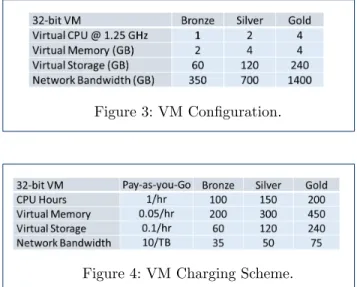
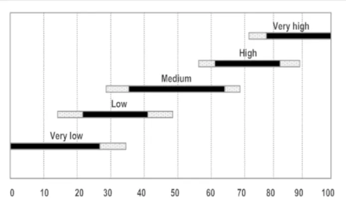
Gold, Silver and Bronze in Figure 3 are names for the different service tiers based on different configura-tions that are commonly used in industry. We can add pricing for Pay-as-you-Go (PAYG) and monthly sub-scription fees to the above scheme to take cost-based selection of configurations into account, see Figure 4.

Figure 3: VM Configuration.

Figure 4: VM Charging Scheme.

We define below a cost functionC:Conf ig→Cost

to formalise such a table. The categories based on the resource workload configurations can now be aligned by the provider with QoS values that are promised in the SLA – here with response time and availabil-ity guarantees filled in the Conf iguration−Quality

matrixCQ:   Gold 0.75 99.99 Silver 1.0 99.9 Bronze 1.5 99   (22)

In general, the Configuration-Quality matrix is de-fined by

CQ= [cij]with i:conf iguration category

and j :quality attribute (23)

A selection functionσdetermines suitable workload patterns Mi for a given quality target qas defined in

the Configuration-Quality matrix and a servicesj:

σ(q, s) ={Mi∈M|M S(q, sj)∈qij} (24)

From this set of workload patterns M1, . . . , Mn, we

determine the most optimal one in terms of resource utilisation. For minimum and maximum utilisation thresholdsminU andmaxU that are derived as

inter-val boundaries from the pattern mining process, the best pattern is selected based on a minimum devia-tion of pattern ranges Mi(q) across all quality factors

(based on the overall mean value) from the threshold average value, defined as the mean average deviation (where xindicates the mean value for any expression

x):

mini

q_X

(maxU −minU−Mi(q))2 (25)

The thresholds can be set at 60% and 80% of the pattern range averages to achieve a good utilisation with some remaining capacity for spikes [15].

Based on the best selected SWP Mi with the given

key metrics, a VM image can be configured accordingly in terms of CPU, storage and network parameters and deployed with the service in question. If several SWPs apply to meet performance requirements, then costs can be considered to select the cheapest offer (if the cost in the table reflects in some way the real cost of provisioned resources and not only charged costs)

σ(q, s)Cost=miniC(σ(q, s)) (26)

for a cost functionC that maps a pattern inσ(q, s) to its cost value. The cost function can create a ranking of otherwise equally suitable patterns or configurations.

The service-based framework presented in Sections 3 and 4 was here applied to the cloud context by link-ing it to standard configuration and payment models. Specific challenges arose from the cloud context that we have addressed are:

• Standard cloud payment models allow an explicit costing, which we took into account here through the cost function. Essentially, the cost function can be used to generate a ranked list of candidate patterns for a required QoS value in terms of the operational cost. In [16], we have demonstrated that different performance result, but also costs vary for a given configuration pattern.

• Cloud solutions are subject to (dynamic) configu-rations, generally both at IaaS and PaaS level. While our configuration here is geared towards typical IaaS attributes, our implementation work with Microsoft Azure (see Section 7) also demon-strates the possibility and benefit of PaaS-level configuration. In [16], we have discussed different PaaS-level storage configurations and their cost and performance implications.

• User-driven scalability mechanisms such as Cloud-Scale or CloudWatch or the AWS Autoscaling typically work on scaling rules defined on the granularity of VMs added/removed. Our solution is based on similar metrics, e.g., GB for storage or network bandwidth, i.e., further automates these solutions.

We have briefly mentioned uncertainties that arise from cloud environments in Section 2. While we have neglected this aspect here so far, [13] presents an ap-proach that adds uncertainty handling on top of pre-diction for VM (re-)configuration, which we will adapt for our problem setting in the next section. Uncertain-ties arise for instance from incomplete or potentially untrusted monitoring data or from varying needs and interpretations of stakeholders regarding quality as-pects. The approach in [13] adds a fuzzy logic pro-cessing on top of a prediction approach.

6 MANAGING UNCERTAINTY

The QoS-SWP matrix captures predictions in the form of mappings or prediction rulesM×S→Qwhere for SWPs in M and services in S as antecedents, we as-sociate quality valuesQas consequents of those rules. Due to the possibly varying number of recorded map-pings and consequently different patterns for different services, there is some uncertainty regarding the re-liability of predictions across the service base caused by possibly insufficient and unrepresentative log data. Sources of uncertainty include:

• at early stages, the amount of log data available is insufficient,

• different monitoring tools provide different log data quality,

• temporary variations in workload might render prediction unreliable.

In order to address these uncertainties, we propose a fuzzy logic-based approach to capture uncertain infor-mation, fuzzify this and infer here quality predictions based on the fuzzified recorded log data.

6.1 Fuzzification of Rule Mappings

The hypothesis that motivates our framework is the observation that utilisation rates for the resources in question (CPU, storage, network) are often subopti-mal. We can look at the Q values in the matrix and find patternsMi _{that run at 60-80% rate for a given}

q∈Q. As we might find a number of possible patterns, a degree of uncertainty emerges as either a number of candidate patterns for a single service or even for a set of similar services might exist.

Our proposal if to fuzzify all pattern mapingsMi×S

and calculate an optimum quality in a fuzzified space before defuzzifying the result as a concrete pattern

with a predicted quality value. Note that this patterns might not be in the pattern-quality matrix, i.e., does not necessarily reflect actual observations. More con-cretely, we fuzzifyM1×M2×M3→Qmappings for one quality range ˜q ∈ Q with ˜q = qmin ∼ qmax and

a given service s∈S. Here, eachMi refers to one of the three aspects CPU, storage and network, result-ing in a set of m patterns with ranges for the three aspects that all map to the same quality range ˜q. The patterns are the different patterns for a service (or a class of similar services) that predict a quality range ˜ q=qmin∼qmax: M1 1..3→q˜ M2 1..3→q˜ · · · Mm 1..3→q˜ (27)

This set will be fuzzified, resulting in joint, fuzzy rep-resentation of the merged patterns.

This technique is based on a fuzzy logic approach to uncertainty that we developed for cloud auto-scaling [13], but adopted here to service quality prediction. The approach is differently applied here in that instead of different linguistic concept definitions used in use-defined auto-scaling rules, we have different (impre-cise) workload ranges. Furthermore, instead of differ-ent scaling actions as rule anteceddiffer-ents, we look at dif-fering performance values (moderately varying). While in [13], we addressed uncertainty regarding human-specified scalability rules, this is uncertainty regarding the monitoring systems and their data.

Here, we obtain data from different, but similar ser-vices via the collaborative filtering technique. Differ-ent associated performances (unpredictable variations caused my factors not considered in the calculation) are determined. Through the variableY, we will later on capture predictions such thatM1_...3

I →q˜∈QThis

can take into account a targeted 60-80% utilisation rate optimum.

In order to simplify the presentation, we only develop the fuzzy logic approach for the CPU processor load as core compute resource, linked to performance at the service level. However, specific characteristics that would distinguish CPU, storage and network do not play any role and, therefore, selecting just one here for simplification does not restrict the solution.

6.2 Fuzzy Logic Definitions for Uncertainty

Fuzzy logic is a suitable tool to reflect the uncertainty that is incorporated in the different patterns for a ser-vice, particularly since these rely on collaborative fil-tering based on similarity with related services.

Fuzzy logic distinguishes different ways to represent uncertainty. A type-1 (T1) fuzzy set associates as a function a possibility value of some attribute, resulting in a single value depending on the input. A type-2 (T2) fuzzy set is an extension of a type-1 (T1) fuzzy set [17]. At a specific valuex0(cf. Figure 5), there is an interval instead of a crisp value for each input.

Figure 5: A type-2 fuzzy set based possibility distribution.

This leads to the definition of a three dimensional membership function (MF), a T2 MF, which charac-terizes a T2 fuzzy set (FS). Note that the core fuzzy logic definitions here are standard definitions in fuzzy theory from the literature such as [18, 19]. Figure 5 visualises the definitions.

A T2 FS, denoted by ˜R , is characterized by a T2 MF µ_R˜(x, u) with

˜

R={((x, u), µ_R˜(x, u)|∀x∈X,∀u∈Jx, µ_R˜(x, u)≤1} (28) When these values have the same weight, it leads to definition of an interval type-2 fuzzy set (IT2 FS):

Ifµ_R˜(x, u) = 1 , ˜Ris an interval T2 FS, also abbre-viated as an IT2 FS.

Therefore, the membership function MF of a IT2 FS can be fully specified by the two boundary T1 MFs. The area between the two MFs (the grey area in Figure 5) characterizes the uncertainty.

The uncertainty in the membership function of an IT2-FS, ˜R, is called footprint of uncertainty (FOU) of

˜

R. Thus, we define:

F OU( ˜R) = [

x∈X

Jx={(x, u)|∀x∈X,∀u∈Jx} (29)

The upper membership function (UMF) and the lower membership function (LMF) of ˜R are two T1-MFs µ_R˜(x) and µ_R˜(x), respectively, that define the boundary of the FOU.

An embedded fuzzy setReis a T1 FS that is located

inside the FOU of ˜R.

6.3 Qualification of Infrastructure Inputs

We need to apply the definitions above to construct IT2 membership functions for our mappings, but first the add labels to ranges in order to work with qualified rather than quantified ranges. This is common in cloud resource configuration.

Assume the following pattern-to-quality mapping with normalised input values in [0..100] for CPU, stor-age and network parameters, respectively:

M₁1_..3= [40−54],[20−26],[30−37]→q˜= [1.1−1.4]

M₁2_..3= [20−33],[26−32],[80−86]→q˜= [0.9−1.3]

M₁3_..3= [16−23],[65−72],[50−55]→q˜= [1.2−1.6]

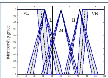
M14..3= [48−56],[71−78],[82−89]→q˜= [1.5−1.9] The ranges above reflect observed CPU utilisation ranges under which the performance is relatively sta-ble. Ranges with similar performance are clustered. We now use a qualified representation of the individual range clusters. For the CPU processor load, we use five individual labels Very Low, Low, Medium, High and Very High. Thus, for the above mapping, we can map the CPU ranges [16-23] to the Very Low label, [20-33] to Low and [40-54] and [48-56] to Medium. The labels themselves are suggested by experts and are commonly used in the configuration of cloud infrastructure solu-tions. While this qualification into concept labels is technically not necessary, these labels help to visualise and communicate the pattern-based prediction to the cloud users.

Figure 6 shows the qualified patterns. For each la-bel, the black bar denotes the variation of the means of each of the pattern value ranges as given by the experts, e.g., the means of [40-54] and [48-56] for the Medium label. The light grey bars denote the overall variation of ranges for each label.

The qualified categorisation will in the next step be used to define fuzzy membership functions that fuzzify the infrastructure input captured in the patterns.

Figure 6: Qualification of Pattern Ranges before Fuzzification.

6.4 Defining Membership Functions

Infrastructure monitoring tools measure the input val-ues for the prediction solution (CPU, storage, net-work) as infrastructure parameters and performance as service-level data). Their conversion to fuzzy values is realized by MFs. In this section, we show how to de-rive appropriate IT2 MFs based on the data extracted from the infrastructure and service monitoring logs. We follow the guidelines in [20] in order to construct the functions. To simplify the investigation, we focus on CPU load and performance only.

As illustrated in Figure 5, we used triangular or trapezoidal MFs to represent different CPU load ranges:

• For each normalized CPU range [CP Umin ∼

CP Umax], we define one type-2 MF as in Figure

7 for five ranges.

• We order these and label them accordingly, e.g., with VL to VH labels representing Very Low to Low, Medium, High and Very High CPU loads.

Figure 7: IT2 Membership Functions for CPU load.

Leta andb be the mean values of the interval end-points CP Umin and CP Umax of the labelled ranges

with standard deviationsσa andσb, respectively (see

Figure 6). For instance, for the Low, Medium and High label, the corresponding triangular T1 MF is then con-structed by connecting leftl, middlemand rightras follows:

l= (a−σa,0), m= ((a+b)/2,1), r= (b+σb,0) (30)

Accordingly, for Very Low and Very High proces-sor load ranges that border 0 or 100% on the nor-malized scale, the associated trapezoidal MFs can be constructed by connecting points as follows:

(a−σa,0),(a,1)(n,1),(b+σb,0) (31)

The labels above refer to utilisation rates of re-sources, with a maximum value being 100. So, irre-spective of the concrete system, the labels are assigned to normalised utilisation ranges.

As indicated by the standard deviations in Figure 6, there are uncertainties associated with the ends and the locations of the MFs. As an example, a triangular T1 MF might be defined follows:

l0 = (a−0.3×σs,0)

m= ((a+b)/2,1)

r0= (b+ 0.4×σb,0)

(32)

These uncertainties cannot be captured by T1 fuzzy MFs. In IT2 MFs on the other hand, the footprint of uncertainty (FOU) can be captured by the upper and lower MFs (UMF and LMF) for each range, see Figure 8. A blurring parameter 0≤α≤1 can determine the FOU (see Figure 6).

Here, we useα= 0.5. Parameterα= 0 reduces IT2 MFs to a T1 MFs, while parameter α = 1 results in fuzzy sets with the widest possible FOUs.

6.5 The Fuzzy Prediction Process

After constructing the IT2 fuzzy sets with the MFs and the set of rules for the infrastructure load patterns, the prediction can then start to determine service quality estimations. The fuzzy prediction technique proceeds in a number of steps as follows (which we will explain in more detail afterwards):

1 The inputs comprising the workload are first fuzzified.

2 Then, the fuzzified input activates an inference mechanism to produce output IT2 FSs.

3 Decisions made through the inference mechanism are represented in the form of fuzzy values, which cannot be directly used as prediction results. The outputs are then processed by a type-reducer, which combines the output sets and subsequently calculates the center-of-set.

4 The type-reduced FSs are T1 fuzzy sets that need to be defuzzified in the last step to determine the predicted quality value q.

5 This valueqis then passed back to the user as the predicted quality.

In the first step, we must specify how the numeric inputs ui ∈Ui for the CPU utilisation rates are

con-verted to fuzzy sets (a process that called ”fuzzifica-tion” [18]) so that they can be used by the FLS. Here, we use singletons:

µR˜1 = (

1 x=ui

0 otherwise (33)

For the defuzzification step, we use the construct of a centroid [21]. The centroid of a IT2 FS ˜Ris the union of the centroids of all its embedded T1 fuzzy setsRe:

C_R˜ ≡

[

∀Re

c(Re) = [cl( ˜R), cr( ˜R)] (34)

For the type-reducing step we use the center-of-sets construct [36]. The center-of-set (cos) type reduction is calculated as follows: Ycos= [ fl_∈Fl_,yl_∈C ˜ Gl ΣN l=1f l_×y1 ΣN l=1fl = [yl, yr] (35)

where fl _{∈ F}l _{is the firing degree of mapping rule l}

and yl _{∈ C}

˜

Gl is the centroid of the IT2 FS ˜Gl. The

centroids cl( ˜R), cr( ˜R) and yl, yr are calculated using

the KM algorithm from [21].

6.6 Fuzzy Reasoning for Quality Prediction

Our quality mappings that encode the SWPs are in a multi-input single-output format. Because the log records of different services may not be similar, many patterns may be conflicting, i.e., we might have rule mappings with the same antecedent, but different con-sequent values. In this step, mappings with the same if-part are combined into a single rule. For each map-ping in the patterns retrieved from the logs, we get the following for a sample rule R1_:

IF (x1 is F1l)and ... and(xp is Fpl),

T HEN (y is y(tlu)₎ (36)

where tl

u is the index for the result. In order to

com-bine these conflicting mappings, we used the average of all the responses for each mapping and use this as the centroid of the mapping consequent. Note, that the mapping consequents are IT2 FSs. However, when the type reduction is used, these IT2 FSs are replaced by their centroids. This means that we represent them as intervals [yn, yn] or crisp values whenyn=yn. This leads to rules with the following form for an arbitrary ruleRl_:

IF the CPU workload (x1) is ˜Fi1,

AND the network load (x2) is ˜Gi2,

AND the storage utilisation (x3) is ˜Hi3,

THEN qi is the predicted value.

whereCis the value of associated consequent, i.e., here a quality value for performance in ms, and wlu is the

weight associated with the u-th consequent of the lth mapping. Therefore, eachqi can be computed.

In a concrete example, we now illustrate the details of the prediction process. Assume that the normal-ized values regarding the three input parameters are

x1 = 40,x2= 50 and x3 = 55, respectively – see the solid lines for the workload in Figure 9 as a sample fac-tor. Forx1= 40, two IT2 FSs for the processor work-load rangesF2=LowandF2=M ediumwith the de-grees [0.3797,0.5954] and [0.3844,0.5434] are fired[1]_. Similarly, for x2 = 50 , three IT2 FSs for the per-formance ranges G3 = M edium, G4 = Slow, and

G5 = V ery Slow with the firing degrees [0,0.1749], [0.9377,0.9568] and [0,0.2212] are fired. For x3 = 55 similar values would emerge. Intuitively, the lower and

[1]_{The term ’fired’ is commonly used for rules, generally}

assuming the consequents of the rules being actions that are fired. We have kept the term, but it applies here only to mappings to quality values.

upper values of the intervals can be computed by find-ing the y-intercept of the solid lines in the Figure, re-spectively, with the LMF and the UMF of the crossed FSs. As a result, six pattern mappings might result that are fired (here a sample is given):

M8: (F2, G3, H1), M9: (F2, G4, H4),

M10: (F2, G5, H4), M13: (F3, G3, H2),

M14: (F3, G4, H1), M15: (F3, G5, H2)

(37)

Figure 9: IT2 MFs of for CPU workload ranges.

The firing intervals are computed using the meet op-eration [17]. For instance, the firing interval associated to the patternM9 for the CPU attribute is:

m9=µ_M˜9 2 (x0₁)⊗µ_˜ G9 4 (x0₂) = 0.3797×0.9377 = 0.3560 (38) The output can be obtained using the center-of-set:

Yl(40,50,55) =

[yl(40,50,55), yr(40,50,55)] =

[0.9296,1.1809]

(39)

The defuzzified output can be calculated as follows:

Y(40,50,55) = 0.9296 + 1.1809

2 = 1.0553 (40) Thus, we can finally calculate the predicted quality

Y(x1, x2, x3) for all the possible normalized values of the input infrastructure parameters (i.e.,x1∈[0,100],

x2 ∈[0,100],x3 ∈[0,100] for CPU, storage and net-work).

7 EVALUATION

Our proposed solution builds on a core pattern-based quality prediction solution that can be used for cloud configuration in an environment where there is uncer-tainty about concerns such as correctness or complete-ness. We have implemented an experimental test en-vironment to evaluate the accuracy, efficiency and ro-bustness of the solution in the context of uncertainty and dynamic processing needs.

7.1 Implementation Architecture and Evaluation Settings

The implementation of the prediction and configura-tion technique covers different parts – off-line and on-line components:

• The pattern determination and the construction of the patterns-quality matrix is done off-line based on monitoring logs. The matrix is needed for dynamic configuration and can be updated as required in the cloud system. For the prediction, the accuracy is central. As the construction is off-line, performance overhead for the cloud environ-ment is, as we will demonstrate, negligible.

• The actual prediction through accessing the ma-trix is done in a dynamic cloud setting as part of a scaling engine that combines prediction and con-figuration. Here the acceptable performance over-head for the prediction needs to be demonstrated.

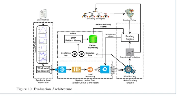
• Uncertainties and noise are additional problems that arise in heterogeneous, cross-organisational cloud architectures. Robustness in the presence of these challenges needs to be demonstrated. For both the accuracy and performance concern, we use a standard prediction solution, collaborative fil-tering (CF) as the benchmark, which is widely used and analysed in terms of these properties, cf. [11] [12] or [5] [6]. We have implemented a simulation envi-ronment with a workload generator to evaluate accu-racy of the prediction approach and the performance of the prediction-based configuration. Test data is de-rived from sources such as [22] where quality met-rics (response time, throughput) are collected for 5825 Web services with 339 users. We selected 100 applica-tion services from three different categories, each cate-gory either sensitive to data size, network throughput or CPU utilization. Figure 10 describes the testbed with the monitoring and SWP extraction solution for Web services. The primary concern is the accuracy of the pattern extraction and pattern-based prediction of performance for deployed services. Furthermore, as dynamic reconfiguration, i.e., auto-scaling, is an aim, also performance needs to be looked at.

We have tested our scalability management in Mi-crosoft Azure. We have implemented a range of stan-dard applications, including an online shopping appli-cation, a services management solution and a video

processing feature to determine the quality metrics for different service and infrastructure configuration types. For the first two, we used the Azure Diagnos-tics CSF to collect monitoring data (Figure 10). We also created an additional simulation environment to gather a reliable dataset without interference from un-controllable cloud factors such as the network. Con-crete applications systems we investigated are the fol-lowing: a single-cloud storage solutions for online shop-ping applications [16] and a multi-cloud HADR solu-tion (high-availability disaster recovery system [23]. This work has resulted in a record of configura-tion/workload data combined with performance data – as for instance shown in [16] where Figs. 3-6 capture response time for different service types and Figs. 7-8 show infrastructure concerns such as CPU and stor-age aspects. In that particular case, 4100 test runs were conducted, using a 3-service application with be-tween 25 and 200 clients requesting services. Azure CSF telemetry was used to obtain monitoring data. This data was then looked at to identify our workload patterns(CPU, Storage, Network)→ Performance.

7.2 Cloud Application Workload Patterns

A number of different application workload patterns are described in the literature [8, 13]. These include static, periodic, one-in-a-lifetime, unpredictable, con-tinuously changing as in [8], or slowly varying, quickly varying, dual phase, steep tri-phase, large variation and big spike [13]. We need to make sure that this experimental evaluation does indeed cover the appli-cation workload pattern in order to guarantee general applicability. We followed [13] and induced these six patterns in our experiments. Based on the successful pattern coverage, we can conclude that the technique is applicable for a range of the most common situa-tions.

We have implemented our prediction mechanism in different platforms. Work we described in [13] deals with how to implement this in an auto-scaling solution such as Amazon AWS where Amazon-monitored work-load and performance auto-scaling metrics are con-sidered together with a prediction of anticipated be-haviour to configure the compute capabilities.

7.3 Accuracy

Reliable performance guarantees based on configura-tion parameters is the key aim – real performance needs to match the expected or promised one for the provider to fulfill the SLA obligations. Accuracy in vir-tualisation environments is specifically challenging [24] due to resource contentions because of the layered ar-chitecture, shared resources and distribution.

Accuracy of prediction is measured in terms of devia-tion from the real behaviour. The metric we use here is

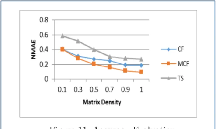
based on themean absolute error(MAE) between pre-diction (SLA imposed) and real response time, which is the normal choice to measure prediction accuracy. Different characteristics of QoS have different ranges. Consequently, we use NMAE (the Normalized Mean Absolute Error) instead of the MAE. The smaller the NMAE, the more accurate is the prediction. We com-pare our solution with similar methods based on tradi-tional prediction methods in terms of matrix density. This covers different situations from situations where little is known about the services (density is low) and situations where there is a reliable base of historic data for pattern extraction and prediction (high density).

Figure 11: Accuracy Evaluation.

In earlier work, we included average-based predica-tions and classical collaborative filtering (CF) in a comparison with our own hybrid method (MCF) of matrix-based matching and collaborative filtering [7]. The NMAE of k = 15 and k = 18 (higher or lower

ks are not interesting as lower values are statistically

not significant and higher ones only show a stabili-sation of the trend) shows an accuracy improvement for our solution compared to standard prediction tech-niques, even without utility function and exponential smoothing, see Figure 11. For this evaluation here, we also include time series (TS) into the comparison. For the evaluation, we considered some noisy data which cannot be in any pattern. We also removed invocation data and then predicted it using the CF, MCF and also the TS time series method from [25].

We can observe that an increase of the dataset size improves the accuracy significantly. In all cases, our MCF approach outperforms the other ones by result-ing in less prediction errors.

7.4 Efficiency Overhead (Runtime)

For automated service management in the context of cloud auto-configuration and auto-scaling we need sufficient performance of the extraction and matching approach itself. To be tested in this context are the performance of three components:

Figure 10: Evaluation Architecture.

1 SWP Extraction from Logs (Matrix Determina-tion)

2 Configuration-Pattern Matching (Existing Pat-terns)

3 Collaborative Filtering (Non-Existing Patterns) For cases 1 and 2, we determined 150 workload pat-terns from 2400 usage recordings. We tested the algo-rithm on a range of different datasets extracted from a number of documented benchmarks and test cases. Com-pared to other work based on the TS and CF solutions, the matrix for collaborative computation is reduced from 2400*100 to 150*100, which reduces ex-ecution time significantly by the factor 16. For case 3, only when a matched pattern provides no information for a target service, the calculation for collaboration prediction is required, see Figure 12, where we com-pare prediction performance with (MCF) as described in Sections 3 and 4 (using Algorithms 1 and 2) and without (CF) the pattern-based matrix utilisation.

7.5 Robustness against Noise and Uncertainty

Exponential smoothing causes noise and results in some unavoidable errors. We need to demonstrate that our prediction solution is resilient against input noises, one of which is the estimation error through smooth-ing.

We experimentally evaluated the robustness against noise. We observed that the worst estimation error happens for large variation and quickly varying pat-terns and is less than 10% of the actual workload. Based on this, we injected a white noise to the input

Figure 12: Performance Evaluation.

measurement data (i.e.,x1) with an amplitude of 10%. We ran RMSE (root-mean-square error – measure of the differences between values predicted by a model or an estimator and the values actually observed) surements for each levels of blurring, and for each mea-surement, we used 10,000 data items as input. We used different blurring values. Two observations emerged:

• Firstly, the error of control output produced by the prediction technique is less than 0.1 for the blurring levels.

• Secondly, the error of control output is decreasing when we configured the technique with a higher blurring.

A higher blurring as part of the smoothing leads to a bigger FOU in the uncertainty management, where

FOU is a representative for the supporting levels of un-certainty. Therefore, the designer should make a choice in terms of the level of uncertainty that is acceptable. Note that in some circumstances an overly wide FOU results in a performance degradation. However, we can state that these observations provide enough evidence that robustness against input noise is maintained. Us-ing IT2 FLS in the uncertainty management actually alleviates here the impact of noise.

7.6 Threats to Validity

Some threats to the validity of the observations here exist. The usefulness of the approach relies on the qual-ity of the workload patterns. While the existence of the patterns can be guaranteed by simply defining the individual ranges in the broadest possible way, thus resulting in some over-arching default patterns, their usefulness will only emerge if they denote sufficiently narrow ranges to allow the resources to be utilised in an equally narrow band. For instance, a band of 60 to 80% is aimed at for processor loads.

While this has emerged to be possible for traditional software services that are computationally intensive or are typical text and static content-driven applications, multi-media type applications for instance with differ-ent network consumption patterns require more inves-tigation.

7.7 Summary of Evaluation

Thus, to conclude the evaluation, the computational effort for the dynamic prediction is decreased to a large extent due to the already partially filled matrix. As already explained, the performance of the pattern extraction and matrix construction (DBSCAN based clustering and collaborative filtering) can be computa-tionally expensive, but can be done offline and only the matrix-based access (as demonstrated in the perfor-mance figure above) impacts on the runtime overhead for the configuration. However, as the results show, our methods overhead increases only slowly even if the data size increases substantially. Consequently, the so-lution in this setting is no more intrusive than a re-active rule-based scalability solution such as Amazon AWS Auto Scaling that would also follow our proposed architecture.

We specifically looked at the accuracy and robust-ness of the solution. The accuracy of the core solu-tion based on the matrix is better than a tradisolu-tional collaborative filtering approach. However, in cloud en-vironments, other concerns needed to be addressed in addition. In order to address uncertainty due to different and possible incomplete and unreliable log data, we added smoothing and fuzzification. We have demonstrated that these features improve the robust-ness against external influence factors.

8 RELATED WORK

QoS-based service selection in general has been widely covered. There are three main categories of prediction-based approaches for selection.

• The first one covers statistical and other mathe-matical methods, which are often adopted for sim-plicity [1] [2] [3] [26] [27]. Others, e.g., in the con-text of performance modeling use mathematical models such as queues.

• The second category selects services based on user feedback and reputation [28] [29]. It can avoid ma-licious feedback, but does not consider the im-pact of SLA requirements and the environment and cannot customise prediction for users.

• The third category is based on collaborative filter-ing [11][12] [30], which is a widely adopted recom-mendation method [31] [32] [33], e.g., [32] summa-rizes the application of collaborative filtering in different types of media recommendation. Here, we combine collaborative filtering with service workload patterns, user requirements and SLA obligations and preferences. This considers differ-ent user preferences and makes prediction person-alized, while maintaining good performance re-sults.

To demonstrate that our solution is an advancement compared to existing work on prediction accuracy, we had singled out two approaches for categories 1 and 3 for the evaluation above.

8.1 General Prediction Approaches

Some works integrate user preferences and user charac-teristics into QoS prediction [11] [12] [30] [5], e.g. [11] [12] propose prediction algorithms based on collabo-rative filtering. They calculate the similarity between users by their usage data and predict QoS based on user similarity. This method avoids the influence of the environment factor on prediction. However, even the same user will have different QoS experiences over time depending on the configuration of the execution environment or will work with different input data. Current work generally does not consider user require-ments. Another current limitation of current solutions is low efficiency as we demonstrated. Our work in [13] is a direction based on fuzzy logic to take user scala-bility preferences into account for a cloud setting.

In [34] [7], pattern approaches are proposed. [34] suggests pattern-based management for cloud config-uration management, but without a detailed solution. [7] is about bottom-up QoS prediction for standard service-based architectures, while in this paper QoS requirements are used to predict suitable workload-oriented configurations taking specifically cloud con-cerns into consideration. We added additionally expo-nential smoothing and utility functions and the cost