an Empirical Analysis of Regularization
Saurav Jha1 Martin Schiemer1 Juan Ye1
Abstract
Given the growing trend of continual learning techniques for deep neural networks focusing on the domain of computer vision, there is a need to identify which of these generalizes well to other tasks such as human activity recognition (HAR). As recent methods have mostly been composed of loss regularization terms and memory replay, we provide a constituent-wise analysis of some prominent task-incremental learning techniques employing these on HAR datasets. We find that most regularization approaches lack substantial effect and provide an intuition of when they fail. Thus, we make the case that the development of continual learning algorithms should be motivated by rather diverse task domains.
1. Introduction
The field of continuous learning for neural networks tries to develop algorithms that mimic the mammalian ability to in-crementally learn new experiences without deterioration of older ones. Sensor-based human activity recognition (HAR) aims to autonomously categorize human activities using a range of sensors such as binary and proximity sensors, ac-celerometers, etc. to gather information about changes of state or physical activities. The use cases are manifold,
rang-ing from smart homes (Zhang et al.,2020) to disease
diagno-sis (Afonso et al.,2019). HAR’s potential benefits from
con-tinuouslearning (often referred to aslifelong/incremental
learning) are obvious: humans dynamically change their be-havior and even develop new activities. Hence, algorithms must adapt to such ever changing diverse behaviors to
pre-vent service quality degradation (Ye et al.,2019). One of the
main stepping stones for continuous learning is that learning a new task interferes with previously acquired knowledge
-1
School of Computer Science, University of St Andrews, St Andrews, Scotland. Correspondence to: Saurav Jha< [email protected]>, Martin Schiemer<[email protected]>.
Proceedings of the37th
International Conference on Machine Learning, Vienna, Austria, PMLR 119, 2020. Copyright 2020 by the author(s).
a phenomenon known ascatastrophic forgetting(CF) (
Mc-Closkey & Cohen,1989). In general, we would prefer that
models arestableenough to retain knowledge while being
plasticenough to incorporate new information (Mermillod et al.,2013). In this paper, we address techniques that try to alleviate CF through regularization.
Algorithms leveraging regularization attempt to alleviate forgetting through the restriction of updates on network parameters. A substantial amount of these have achieved significant progress on image datasets, it is important to verify their generalization capabilities to other domains
such as HAR which is marked by: (i)dataset imbalance
– frequencies of activities can vary a lot with some being
recurring while others rare; (2)inter-class similarity–
ac-tivities might resemble each other thus forming overlapping
inter-class boundaries; (3)intra-class diversity– an
activ-ity can be performed in different ways; and (4)resource
constraints– most HAR systems are deployed on mem-ory and computation-constrained devices such as wearables. Characteristics of the sensor datasets used, can be found in
AppendicesBandC.
The main contribution of our work lies in assessing the appli-cability and pitfalls of notable continual learning techniques
on HAR1. Even though a high volume of continual learning
techniques have been proposed in recent years, we focus on regularization and memory replay (MemR) techniques. We are not considering dynamic architecture approaches as HAR systems might not get to see a large number of classes (e.g., around 10-30).
We select five regularization-based methods, which range
from classic methods such as LwF (Li & Hoiem,2016) and
EWC (Kirkpatrick et al.,2016), to more recent methods such
as MAS (Aljundi et al.,2018), LUCIR (Hou et al.,2019) and
ILOS (He et al.,2020). We assess these techniques on two
third-party, publicly available datasets that are representative
in two common sensor families:accelerometerandambient
sensors. Through an empirical evaluation on these datasets, we conclude that the regularization terms often have little or even detrimental effect in our scenarios (esp. together
1
Code will be made available athttps://github.com/
with memory replay) and may sometimes be worse than the lower boundary of applying plain cross-entropy (CE) loss.
2. Techniques
This section will briefly introduce the regularization terms
whose description can be found in AppendixA.LwF
em-ploys knowledge-distillation (KD) loss (Hinton et al.,2015)
to continuous learning with an objective of maintaining the logits of an incremental step model similar to its
pre-decessor. EWCapproximates the posterior distribution of
network parameters and uses it to identify their importance
and penalize their updates. Rotated EWC (RWC) (Liu et al.,
2018) improves upon EWC by addressing its assumption
that fisher information matrix in the network’s parameter space are diagonal. Since this is often not the case, they rotate the parameter space in a manner that it does not alter
the feed-forward response of the network.MAScalculates
the importance of parameters by approximating the change in the network output caused by perturbations in parameters
due to training on the new task data.LUCIRintroduces two
loss terms:less forget constraint(DIS) andmargin ranking
(MR)2 with the goals of preventing rotation of old class
embeddings and reducing ambiguities between old and new
classes. ILOSmodifies the CE loss by replacing the new
model’s logits for old classes with those adjusted propor-tionately between new and previous model. They coin the resultant loss as cross-distillation loss. We also consider lower bound as the model trained with CE loss and upper bound as the offline training with all tasks at the same time.
The CE loss is defined asLCE(y,yˆ) =−Pylog ˆy, where
y and andyˆare the ground truth and output logits for an
input sample.
3. Experimental Setup
Our main objective is to assess which type of regularization term is effective for continual learning on sensor-based HAR and to what degree.
3.1. Datasets
We select two datasets from the sensor-based HAR
commu-nity. The first dataset(WS)was collected on 32 ambient
passive infra-red sensors by a smart home testbed at the
Washington State University’s CASAS.3It includes 9
imbal-anced activities: cooking, eating, leaving/entering the house, living room activity, toilet use, mirror, reading, sleeping, and
working. The second dataset isDSADS– Daily and Sports
Activities Dataset (Altun & Barshan,2010). It is a balanced
dataset with 19 activities that include sitting, running on a 2
MR only applies to memory replay since in-memory samples are used to distance class embeddings.
3
http://ailab.wsu.edu/casas/datasets/
treadmill, exercising on a stepper, and rowing among others - each of which is performed by 8 subjects for 5 minutes with 5 accelerometer units on a subject’s torso, right arm, left arm, right leg and left leg. Circumventing the topic of feature extraction, we work on the features already extracted by prior work instead of the raw spatio-temporal sensor data.
For DSADS, we use a version processed byWang et al.
(2018) which extracts 27 features (including mean, standard
deviation, and correlations on axes) on each sensor. For WS,
we use those generated byFang et al.(2020).
3.2. Evaluation Process
Considering task order-sensitivity in continual learning
paradigms (Yoon et al.,2019), we evaluate the techniques on
30 task sequences while updating the parameters on every incoming task. Each task is coupled with two randomly
sam-pled classes, thus contributing to a sequence length of|C|/2,
where|C|is the total number of classes in the dataset.
We perform a stratified train-test split of 70/30 on WS dataset while for DSADS, we split data on participants;
i.e.,we use data from 70% of subjects for training and the
remaining 30% for testing. After training, we retain |CS∗||seenC|
random samples per class in the memory to be replayed at
further incremental training steps. Sis determined by the
memory constraint of the HAR system and|C|seenis the
number of classes observed till the current incremental step.
3.3. Evaluation Metrics
Upon arrival of a new task k, we compute four types of
accuracy: baseand old class accuracies measure
perfor-mance on the very first (0th) task and the tasks{1, .., k−1}
henceforth, thus indicating thestabilityof the model;new
accuracy measures the performance on the current task thus
indicating the plasticity of the model; andoverall
accu-racy considers all the tasks learned so far, and implies the
stability-plasticitybalance of the model. The accuracy is measured in micro-F1 scores. Given the imbalanced class
distribution in a real-world HAR scenario (see AppendixC),
we additionally report macro-F1 scores.
For discerning the preservation of existing knowledge, we
calculate theforgetting measureproposed byChaudhry et al.
(2018) which for taskkis the difference between its
maxi-mum accuracy seen so far and the current accuracy averaged over{1, .., k−1}tasks:Fk =k−11Pkj=1−1ak,j,max−ak,j.
3.4. Model Configuration and Hyperparameter Tuning
Irrespective of their original works, we maintain a com-mon network architecture across all our experiments as a fair comparison premise. We use fully-connected feed-forward networks with the following specifications opti-mized through extensive grid search: (1) DSADS: 3 hidden
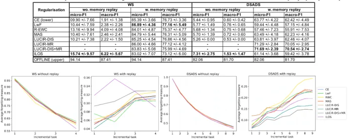
Table 1.Performance comparison of different regularization terms.wo.andw.refer towithoutandwithmemory replay respectively.
micro-F1 macro-F1 micro-F1 macro-F1 micro-F1 macro-F1 micro-F1 macro-F1
CE (lower) 09.90 +/- 7.66 1.91 +/- 1.38 85.39 +/- 3.66 76.73 +/- 3.36 5.44 +/- 0.95 0.60 +/- 0.42 63.77 +/- 4.22 62.42 +/- 4.49 LwF 10.44 +/- 7.59 2.38 +/- 2.26 86.89 +/- 4.36 77.16 +/- 5.49 5.77 +/- 1.49 0.76 +/- 0.65 59.44 +/- 4.48 57.15 +/- 4.84 R-EWC 13.16 +/- 9.94 4.09 +/- 4.08 84.01 +/- 4.87 75.37 +/- 4.77 5.68 +/- 1.34 0.75 +/- 0.68 57.46 +/- 7.23 55.91 +/- 7.53 MAS 10.40 +/- 7.61 2.46 +/- 2.41 84.79 +/- 5.44 76.31 +/- 5.09 5.70 +/- 1.39 0.72 +/- 0.60 63.49 +/- 4.18 62.23 +/- 4.16 LUCIR-DIS 10.21 +/- 7.38 2.22 +/- 1.50 85.25 +/- 4.54 76.86 +/- 4.56 5.26 +/- 0.00 0.53 +/- 0.00 63.81 +/- 3.97 62.46 +/- 4.07 LUCIR-MR - - 86.00 +/- 4.66 77.12 +/- 4.12 - - 71.29 +/- 2.84 70.05 +/- 2.95 LUCIR-DIS+MR - - 83.83 +/- 5.08 75.99 +/- 4.69 - - 71.69 +/- 2.39 70.54 +/- 2.74 ILOS 15.74 +/- 9.57 6.22 +/- 5.67 83.02 +/- 7.07 73.12 +/- 6.00 7.31 +/- 2.75 1.53 +/- 1.47 61.14 +/- 3.68 59.42 +/- 3.78 OFFLINE (upper) 94.14 87.41 94.14 87.41 82.06 81.70 82.06 81.70 Regularisation WS DSADS
wo. memory replay w. memory replay wo. memory replay w. memory replay
Figure 1.Forgetting measure comparison of losses with and without memory replay.
layers of sizes [202, 202, 101], and (2) WS: 2 hidden layers of sizes [32, 16, 16]. Each network has a single output head that gets extended on each incoming task to accommodate for new classes.
We perform a further search for technique-specific
hyper-parameters, detailed in AppendixD. It is worth noting that
our LUCIR-based losses employ L2 normalization of the output logits of FC layer rather than the cosine normaliza-tion which offers a significant boost to performance in the
original work ofHou et al.(2019). This compliments our
fair premise assumption of assessing regularization alone.
4. Results
Fixed holdout size: Table 1 compares the micro and macro-F1 scores of regularization terms on WS and DSADS
with and without MemR. The replay-based scores useS= 6
which we assume to be small enough to be held in a resource-constrained device and large enough to deliver decent perfor-mance. We find that most of the regularization techniques when devoid of replay only achieve the naive accuracy of baseline CE. In this scenario, ILOS with a direct influence of logits from the old model performs better than the rest where the models learn to align them as training progresses. When aided with replay, we find that CE alone beats most of the other techniques on both the datasets. For example, the improvements over the baseline CE approach remain within 1% on the WS dataset and within 8% on the DSADS dataset on both micro and macro-F1. We further observe that LUCIR’s less-forget-constraint (DIS) does not provide a strong effect.
In terms oftask order-sensitivitywithout MemR,
LUCIR-DIS with the least average standard deviation has a clear win over the rest of the methods while ILOS and RWC offer less robustness. When MemR is used, the picture is more diverse between datasets as LwF and LUCIR-DIS+MR are the most stable for WS and DADS respectively.
We see that the differences between the F1 micro and macro scores vary across the methods. For the results without MemR, the micro scores are multiple times higher with CE being the most divergent (518% and 907%) while ILOS the
least (253% and 448%). Table3in AppendixEpresents the
divergence scores between F1-micro and macro. From this, we conclude that the regularization methods help in learning fairer distributions of classes. In contrast, the advantage of the regularization methods with MemR is less apparent with no big difference to CE.
Forgetting: Figure1depicts the stark contrast of
forget-ting scores (F) of replay-assisted techniques to those
with-out replay. Withwith-out MemR,Fdecreases sharply below 1.0
across all methods as the learning progresses beyond task 1. Although the strikingly high forgetting scores stipulate catastrophic forgetting on earlier tasks, these further shed
light into thestabilityof techniques that are devoid of
re-play as their forgetting diminish with the arrival of further diverse tasks. On the other hand, the contribution of the regularization terms improve from being null to modest with MemR. In particular, we observe a threshold number of in-cremental tasks for replay-assisted methods following which the inertia of forgetting dampens. ILOS, LUCIR-MR and LUCIR-DIS+MR attain this threshold much earlier than CE. The high forgetting scores of RWC conform to the finding of
Figure 2.F1 performance comparison of different in-memory sizes. WS F1 scores on the left, DSADS on the right.
at learning new categories incrementally. LwF and ILOS start with relatively larger forgetting scores whose slope alleviates with further incremental steps. In contrast, mar-gin ranking-based techniques have lesser overall forgetting scores, which accords with greater inter-class separation between and old and new classes.
2 3 4 5 80 82 84 86 88 90 92 94 96 Base 2 3 4 5 80 82 84 86 88 90 92 94 96 Old 2 3 4 5 40 50 60 70 80 90 100 New 2 3 4 5 77.5 80.0 82.5 85.0 87.5 90.0 92.5 95.0 All WS: CE LwF RWC MAS LUCIR-DIS LUCIR-MR LUCIR-DIS+MR ILOS No. of tasks Micro-F1 (%) 2 3 4 5 6 7 8 910 50 60 70 80 90 Base 2 3 4 5 6 7 8 910 55 60 65 70 75 80 85 90 95 Old 2 3 4 5 6 7 8 910 20 30 40 50 60 70 80 90 100 New 2 3 4 5 6 7 8 910 60 65 70 75 80 85 90 95 All DSADS: CE LwF RWC MAS LUCIR-DIS LUCIR-MR LUCIR-DIS+MR ILOS No. of tasks Micro-F1 (%)
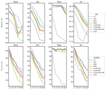
Figure 3.Accuracies detailed by base, old, new and all classes per incremental task.
Performance across base, new and old classes: While LUCIR-DIS+MR and LwF outperform other techniques on DSADS and WS respectively on overall tasks, an
observa-tion of the base, new and old class accuracies in Figure3
offers additional insights into how different techniques
re-spond to theplasticity-stabilitytrade-off. ILOS, for instance,
consistently performs poorer on new classes across both the data sets. However, the maximum scores of ILOS on base and old classes make it more robust to interferences due to new knowledge hence showing that even a direct tuning of the new model’s logits based on the previous model can help surpass complex regularization operations. Together with this and the divergences between F1 macro and micro scores, we assume that ILOS’s restrictiveness for new classes ac-tually harms the learning when used in conjunction with
MemR. We also observe that margin-ranking based methods (LUCIR-MR and LUCIR-DIS+MR) perform poorer than others on new tasks but are robust at preserving old knowl-edge. An intuitive explanation to this could be the design of MR that reinforces the model’s confidence at recognizing ground truth embeddings for old class samples following multiple incremental training steps.
Varying holdout sizes: Drawing inspiration from the su-perior performance of replay-assisted learning, we further
evaluate these forS ∈ {2,4,6,8,10,15}. Figure2shows
that even a small number of replay samples can yield a huge leap in the performance of the techniques than when ran
without replay (Table1). For WS, we see that the majority
of the methods react in the same way to memory upgrades as their F1 scores start with a similar slope and reach a com-parable pace starting from step 4. A few of them stick out: ILOS which mostly has a lower score than the rest but the slope is similar. LUCIR-DIS+MR reaches the level of most methods later and is less stable. We attribute these anoma-lies to the imbalanced sample distribution of WS. Looking at the results on DSADS which has perfectly balanced class distribution, this seems to be the case as we can see an al-most linear increase in score with rising memory. Thus, we conclude that the working of regularization terms is more dependent on dataset characteristics than on the available memory.
5. Conclusion
In this paper, we have shown that the well known continuous learning regularization terms have no or only limited effect in human activity recognition scenarios when used with or without memory replay.
Memory replay, in particular, overshadows the value of regularization and some techniques even adversely affect the learning process. Most importantly, we advocate that the direction of continual learning research should not only focus vision tasks but also target other domains with diverse data distribution and resource constraints.
References
Afonso, L. C., Rosa, G. H., Pereira, C. R., Weber, S. A., Hook, C., Albuquerque, V. H. C., and Papa, J. P. A recurrence plot-based approach for Parkinson’s disease
identification. Future Generation Computer Systems,
2019. ISSN 0167739X. doi: 10.1016/j.future.2018.11. 054.
Aljundi, R., Babiloni, F., Elhoseiny, M., Rohrbach, M., and Tuytelaars, T. Memory Aware Synapses: Learning What
(not) to Forget.ECCV, 2018.
Altun, K. and Barshan, B. Human Activity Recognition
Using Inertial/Magnetic Sensor Units. InProceedings of
the First International Conference on Human Behavior Understanding, HBU’10, pp. 38–51, Berlin, Heidelberg, 2010. Springer-Verlag. ISBN 3-642-14714-3,
978-3-642-14714-2. URLhttp://dl.acm.org/citation.
cfm?id=1881331.1881338.
Chaudhry, A., Dokania, P. K., Ajanthan, T., and Torr, P. H. Riemannian Walk for Incremental Learning:
Un-derstanding Forgetting and Intransigence. In Lecture
Notes in Computer Science (including subseries Lec-ture Notes in Artificial Intelligence and LecLec-ture Notes in Bioinformatics), 2018. ISBN 9783030012519. doi: 10.1007/978-3-030-01252-6 33.
Fang, L., Ye, J., and Dobson, S. Discovery and Recogni-tion of Emerging Human Activities Using a Hierarchical
Mixture of Directional Statistical Models.IEEE
Transac-tions on Knowledge and Data Engineering, 32(7):1304– 1316, jul 2020. ISSN 1041-4347. doi: 10.1109/TKDE.
2019.2905207. URLhttps://ieeexplore.ieee.
org/document/8667728/.
He, J., Mao, R., Shao, Z., and Zhu, F. Incremental Learning
In Online Scenario. mar 2020. URLhttp://arxiv.
org/abs/2003.13191.
Hinton, G., Vinyals, O., and Dean, J. Distilling the
Knowledge in a Neural Network. mar 2015. URL
http://arxiv.org/abs/1503.02531.
Hou, S., Pan, X., Loy, C. C., Wang, Z., and Lin, D. Learning
a unified classifier incrementally via rebalancing. In
Pro-ceedings of the IEEE Computer Society Conference on Computer Vision and Pattern Recognition, 2019. ISBN 9781728132938. doi: 10.1109/CVPR.2019.00092.
Kemker, R., McClure, M., Abitino, A., Hayes, T. L., and Kanan, C. Measuring catastrophic forgetting in neural
networks. InThirty-second AAAI conference on artificial
intelligence, 2018.
Kirkpatrick, J., Pascanu, R., Rabinowitz, N., Veness, J., Desjardins, G., Rusu, A. A., Milan, K., Quan, J., Ra-malho, T., Grabska-Barwinska, A., Hassabis, D., Clopath, C., Kumaran, D., and Hadsell, R. Overcoming catas-trophic forgetting in neural networks. dec 2016. URL
http://arxiv.org/abs/1612.00796.
Li, Z. and Hoiem, D. Learning Without Forgetting. In
European Conference on Computer Vision 2016, pp. 614–629. 2016. doi: 10.1007/978-3-319-46493-0 37. URL http://link.springer.com/10.1007/ 978-3-319-46493-0{_}37.
Liu, X., Masana, M., Herranz, L., Van De Weijer, J., Lopez, A. M., and Bagdanov, A. D. Rotate your Networks: Better Weight Consolidation and Less Catastrophic Forgetting. InProceedings - International Conference on Pattern Recognition, 2018. ISBN 9781538637883. doi: 10.1109/ ICPR.2018.8545895.
MacKay, D. J. C. A Practical Bayesian Framework for
Backpropagation Networks. Neural Computation, 1992.
ISSN 0899-7667. doi: 10.1162/neco.1992.4.3.448. McCloskey, M. and Cohen, N. J. Catastrophic
Interfer-ence in Connectionist Networks: The Sequential
Learn-ing Problem. Psychology of Learning and Motivation
-Advances in Research and Theory, 1989. ISSN 00797421. doi: 10.1016/S0079-7421(08)60536-8.
Mermillod, M., Bugaiska, A., and Bonin, P. The stability-plasticity dilemma: investigating the continuum from catastrophic forgetting to age-limited learning effects.
Frontiers in Psychology, 2013. ISSN 1664-1078. doi: 10.3389/fpsyg.2013.00504.
Wang, J., Chen, Y., Hu, L., Peng, X., and Yu, P. S. Stratified Transfer Learning for Cross-domain Activity Recognition. In 2018 IEEE International Conference on Pervasive Computing and Communications, PerCom 2018, 2018. ISBN 9781538632246. doi: 10.1109/PERCOM.2018. 8444572.
Ye, J., Dobson, S., and Zambonelli, F. Lifelong Learning
in Sensor-Based Human Activity Recognition. IEEE
Pervasive Computing, 2019. ISSN 15582590. doi: 10. 1109/MPRV.2019.2913933.
Yoon, J., Kim, S., Yang, E., and Hwang, S. J. Scalable and Order-robust Continual Learning with Additive Parameter
Decomposition. arXiv e-prints, art. arXiv:1902.09432,
February 2019.
Zhang, Y., Tian, G., Zhang, S., and Li, C. A Knowledge-Based Approach for Multiagent Collaboration in Smart Home: From Activity Recognition to Guidance Service.
IEEE Transactions on Instrumentation and Measurement, 2020. ISSN 15579662. doi: 10.1109/TIM.2019.2895931.
A. Loss Function Terms
LwF uses knowledge distillation loss to approximate the
output of the original network:
LKD(yo,yˆo) =− l
X
i=1
y0o(i)log ˆyo0(i), (1)
wherel is the number of class labels, andy
0(i)
o andyˆ
0(i) o
are temperature-scaledrecordedandcurrentprobabilities
of the sample on a label l. The loss LKD is combined
with the cross-entropy loss on new task samples to form the
cross-distillationloss:
L(yn,yˆn, yo,yˆo) =λoLKD(yo,yˆo) +LCE(yn,yˆn) (2)
whereλois a loss balance weight computed as the ratio of
old classes to total observed classes. A largerλofavors the
old task performances over new task.
EWC assumes that if a datasetDconsists of two
inde-pendent tasks A and B, then the importance of
param-eters of the model is modeled as the posterior
distribu-tionlogp(θ|D) =logp(DB|θ) +logp(θ|DA)−logp(DB).
p(θ|DA)suggests which parameters are important to taskA.
The true posterior probabilityp(θ|DA)is intractable, and
thus it is estimated via Laplace approximation (MacKay,
1992) with precision determined by the Fisher Information
Matrix (FIM). The loss function for EWC is defined as:
L(θ) =LB(θ) + X i λ 2Fi(θi−θ ∗ A,i) 2, (3)
whereLBis the loss on task B,λindicates the importance of
the old task with respect to the new task, andiis the
param-eter index.RWCimproves upon EWC by reparameterizing
θthrough rotation in a way that it does not change outputs
of the forward pass but the FIM computed from gradients during the backward pass is approximately diagonal.
MAS considers approximating the importance of a
net-work’s parameters by learning the sensitivity of the
objec-tive function to a parameter change;i.e.,given a data point
xkwhose network output isF(xk;θ), a change in the
net-work output caused by a small perturbationδ = {δij}
in the parameters θ = {θij} can be approximated as:
F(xk;θ+δ)−F(xk;θ)≈P i,j
gij(xk)δij, wheregis the
gradient with respect to the parameterθ, andgij(xk) =
∂(F(xk,θ)
∂θij . Accumulating gradients over all the data points,
the importance weight on a parameterθijcan be computed
as: Ωij = N1
N
P
k=1
||gij(xk)||. While learning a new task,
MAS then defines the loss function as: L(θ) =Ln(θ) + λ 2 X i,j Ωij(θij−θ∗ij) 2 , (4)
whereLn(θ)is the loss on the new task,θij andθ∗ijare the
new and old network parameters, andλis a hyperparameter
that varies with the dataset.
LUCIR primarily targets theclass imbalancearising due to a small amount of in-memory samples of old tasks and a large amount of samples of new tasks in the data of an incremental training step. This is tackled using two kinds
of losses: (i)less-forget constraintloss (LG
dis) is introduced
to preserve the spatial configuration of old classes’ em-beddings by encouraging the features extracted from the new model to be rotated in the direction similar to those
of the old model,i.e.,LG
dis(x) = 1− hf˜∗(x),f˜(x)i, where
˜
f(x)andf˜∗(x)are normalised features extracted by the
new and the old model respectively, andhv1, v2idenotes
the cosine similarity between the vectorsv1 andv2; (ii)
margin ranking(Lmr) loss is used to enhance inter-class separation by pushing the ground-truth old classes for each
in-memory samplexfar from all new classes it is confused
with. To achieve this, the logits of ground-truth classes of
xare treatedpositivewhile the logits of top-K classes that
xis most confused with are treated as hardnegatives,i.e.,
Lmr(x) = K
P
k=1
max(m−hθ˜(x),f˜(x)i+hθ˜k.f˜(x)i,0). The
loss function resulting from the combination ofLG
disand
Lmrcan be given as:
L= 1 |N| X x∈N (Lce(x) +λLGdis(x)) + 1 |No| X x∈No Lmr(x), (5)
whereN is a training batch drawn fromX andNo
repre-sents the reserved old samples.λis a hyperparameter that
says how much knowledge of the previous model needs to be preserved depending on how many new classes are
introduced and is computed by multiplying a fixedλbase
with the squared root of the fraction of new and old classes;
i.e.,λ=λbase
p
|CN|/|Co|.
ILOS uses an accommodation ratio0≤β≤1to adjust
the proportion of logits from the current model and the previous model: ˜ ok = ( βok+ (1−β) ˆok 1≤k≤n ok, n+ 1≤k≤n+m (6)
wherenis the number of classes observed till previous task,
mis the number of classes in the current task,o˜kare the
adjusted output logits andoˆkare the output logits from the
FC layer of the previous model. The adjusted norms of old classes are thus inclined either towards the range of norms of old classes of the current model or that of the previous model. The degree of this inclination is proportional to the
magnitude ofβ. WhileLKDin Equation2is still calculated
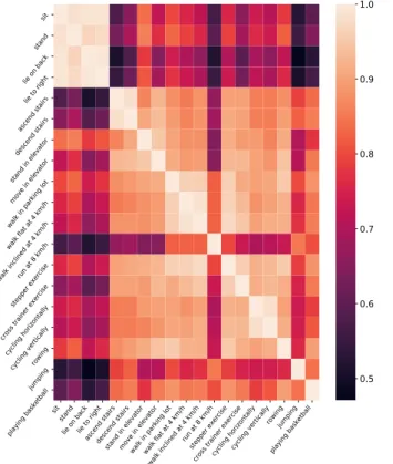
B. Inter-class Similarity
Figure4shows the correlation among raw features of
ac-tivities in DSADS. Due to bodily restrictions and subject-specific fashion, different activities might have resemblance in distribution.
sit stand
lie on backlie to right ascend stairsdescend stairs
stand in elevatormove in elevatorwalk in parking lotwalk flat at 4 km/h walk inclined at 4 km/h
run at 8 km/h stepper exercise
cross trainer exercisecycling horizontallycycling vertically rowingjumping playing basketball sit stand lie on back lie to right ascend stairs descend stairs stand in elevator move in elevator walk in parking lot walk flat at 4 km/h walk inclined at 4 km/hrun at 8 km/h stepper exercise cross trainer exercise cycling horizontally cycling verticallyrowing jumping playing basketball 0.5 0.6 0.7 0.8 0.9 1.0
Figure 4.Correlation heatmap of activities in the DSADS ac-celerometer dataset.
C. Class distribution
As shown in Figure5, the two datasets used in our work
represent two different scenarios of class distribution apart from having captured using different sensor technologies.
D. Technique-specific hyperparameters
This is a brief overview over the hyperparameters derived
by grid search.λfor LwF, RWC and MAS are set to 1.6, 3
and 0.25 each. LUCIR-based losses use aλbase= 5, and
mandkfor LUCIR-MR are set to 0.5 and 2 each.
Table 2.Additional experiment hyperparameters
Dataset WS DSADS
Batch size 15 20
Initial Learning Rate 0.01 0.01
Epochs till Convergence 200 200
Learning Rate Scheduler Step Size (effective after) 40 (50)4
50 (50)
Weight Decay Rate 1.00E-04 1.00E-04
0
1
2
3
4
5
6
7
8
Activity ID
0
40
80
120
160
Count
(a) WS1.0
2.0
3.0
4.0
5.0
6.0
7.0
8.0
Person ID
0
150
300
450
600
750
900
1050
Count
Activity ID1
2
3
4
5
6
7
8
9
10
11
12
13
14
15
16
17
18
19
(b) DSADSFigure 5.Frequency distribution of activities in WS and DSADS datasets.
E. Relative Divergence between F1 Micro and
Macro Scores
Table 3.F1-Micro / F1-Macro in percent (%). Method WS Blank WS Memory Replay DSADS Blank DSADS Memory Replay
CE 518.32 111.29 906.67 102.16 LwF 438.66 112.61 759.21 104.01 RWC 321.76 111.46 757.33 102.77 MAS 422.76 111.11 791.67 102.02 LUCIR-DIS 459.91 110.92 992.45 102.16 LUCIR-MR - 111.51 - 101.77 LUCIR-DIS+MR - 110.32 - 101.63 ILOS 253.05 113.54 477.78 102.89 4
For example, learning rate for training on WS reduces by a factor of 0.01 after 90, 130 and 170 epochs.