Contents lists available atScienceDirect
Expert Systems With Applications
journal homepage:www.elsevier.com/locate/eswaFeature selection using Joint Mutual Information Maximisation
Mohamed Bennasar, Yulia Hicks, Rossitza Setchi
∗School of Engineering, Cardiff University, Cardiff CF24 3AA, UK
a r t i c l e
i n f o
Keywords: Feature selection Mutual information Joint mutual information Conditional mutual information Subset feature selection Classification
Dimensionality reduction Feature selection stability
a b s t r a c t
Feature selection is used in many application areas relevant to expert and intelligent systems, such as data mining and machine learning, image processing, anomaly detection, bioinformatics and natural language processing. Feature selection based on information theory is a popular approach due its computational ef-ficiency, scalability in terms of the dataset dimensionality, and independence from the classifier. Common drawbacks of this approach are the lack of information about the interaction between the features and the classifier, and the selection of redundant and irrelevant features. The latter is due to the limitations of the employed goal functions leading to overestimation of the feature significance.
To address this problem, this article introduces two new nonlinear feature selection methods, namely Joint Mutual Information Maximisation (JMIM) and Normalised Joint Mutual Information Maximisation (NJMIM); both these methods use mutual information and the ‘maximum of the minimum’ criterion, which alleviates the problem of overestimation of the feature significance as demonstrated both theoretically and experimentally. The proposed methods are compared using eleven publically available datasets with five competing methods. The results demonstrate that the JMIM method outperforms the other methods on most tested public datasets, reducing the relative average classification error by almost 6% in comparison to the next best performing method. The statistical significance of the results is confirmed by the ANOVA test. More-over, this method produces the best trade-off between accuracy and stability.
© 2015 The Authors. Published by Elsevier Ltd. This is an open access article under the CC BY-NC-ND license (http://creativecommons.org/licenses/by-nc-nd/4.0/).
1. Introduction
High dimensional data is a significant problem in both super-vised and unsupersuper-vised learning (Janecek, Gansterer, Demel, & Ecker, 2008), which is becoming even more prominent with the recent ex-plosion of the size of the available datasets both in terms of the num-ber of data samples and the numnum-ber of features in each sample (Zhang et al., 2015). The main motivation for reducing the dimensionality of the data and keeping the number of features as low as possible is to decrease the training time and enhance the classification accuracy of the algorithms (Guyon & Elisseeff, 2003; Jain, Duin, & Mao, 2000; Liu & Yu, 2005).
Dimensionality reduction methods can be divided into two main groups: those based on feature extraction and those based on feature selection. Feature extraction methods transform existing features into a new feature space of lower dimensionality. During this process, new features are created based on linear or nonlinear combinations of features from the original set. Principal Component Analysis (PCA)
∗ Corresponding author. Tel: +44 2920875720; fax: +44 2920874716.
E-mail addresses:[email protected](M. Bennasar),[email protected](Y. Hicks), [email protected](R. Setchi).
(Bajwa, Naweed, Asif, & Hyder, 2009; Turk & Pentland, 1991) and Linear Discriminant Analysis (LDA) (Tang, Suganthana, Yao, & Qina, 2005; Yu & Yang, 2001) are two examples of such algorithms. Feature selection methods reduce the dimensionality by selecting a subset of features which minimises a certain cost function (Guyon, Gunn, Nikravesh, & Zadeh, 2006; Jain et al., 2000). Unlike feature extraction, feature selection does not alter the data and, as a result, it is the preferred choice when an understanding of the underlying physical process is required. Feature extraction may be preferred when only discrimination is needed (Jain et al., 2000).
Feature selection is used in many application areas relevant to ex-pert and intelligent systems, such as data mining and machine learn-ing, image processlearn-ing, anomaly detection, bioinformatics and natural language processing (Hoque, Bhattacharyya, & Kalita, 2014). Feature selection is normally used at the data pre-processing stage before training a classifier. This process is also known as variable selection, feature reduction or variable subset selection.
The topic of feature selection has been reviewed in detail in a number of recent review articles (Bolón-Canedo, Sánchez-Maroño, & Alonso-Betanzos, 2013; Brown, Pocock, Zhao, & Lujan, 2012; Chandrashekar & Sahin, 2014; Vergara & Estévez, 2014). Usually, feature selection methods are divided into two categories in terms of http://dx.doi.org/10.1016/j.eswa.2015.07.007
0957-4174/© 2015 The Authors. Published by Elsevier Ltd. This is an open access article under the CC BY-NC-ND license (http://creativecommons.org/licenses/by-nc-nd/4.0/).
evaluation strategy, in particular, classifier dependent (‘wrapper’ and ‘embedded’ methods) or classifier independent (‘filter’ methods). Wrapper methods search the feature space, and test all possible subsets of feature combinations by using the prediction accuracy of a classifier as a measure of the selected subset’s quality, with-out modifying the learning function. Therefore, wrapper methods can be combined with any learning machine (Guyon et al., 2006). They perform well because the selected subset is optimised for the classification algorithm. On the other hand, wrapper methods may suffer from over-fitting to the learning algorithm. This means that any changes in the learning model may reduce the usefulness of the subset. In addition, these methods are very expensive in terms of computational complexity, especially when handling extremely high-dimensional data (Brown et al., 2012;Cheng et al., 2011;Ding & Peng, 2003; Karegowda, Jayaram, & Manjunath, 2010).
The feature selection stage in the embedded methods is combined with the learning stage. These methods are less expensive in terms of computational complexity and less prone to over-fitting; however, they are limited in terms of generalisation, because they are very spe-cific to the used learning algorithm (Guyon et al., 2006).
Classifier-independent methods rank features according to their relevance to the class label in the supervised learning. The relevance score is calculated using distance, information, correlation and consistency measures. Many techniques have been proposed to compute the relevance score, including Pearson correlation coef-ficients (Rodgers & Nicewander, 1988), Fisher’s discriminate ratio “Fscore” (Lin, Li, & Tsai, 2004), the Scatter criterion (Duda, Hart, & Stork, 2001), Single Variable Classifier SVC (Guyon & Elisseeff, 2003), Mutual Information (Battiti, 1994), the Relief Algorithm (Kira & Rendell, 1992; Liu & Motoda, 2008), Rough Set Theory (Liang, Wang, Dang, & Qian, 2014) and Data Envelopment Analysis (Zhang, Yang, Xiong, Wang, & Zhang, 2014).
The main advantages of the filter methods are their computa-tional efficiency, scalability in terms of the dataset dimensionality, and independence from the classifier (Saeys, Inza, & Larranaga, 2007). A common drawback of these methods is the lack of information about the interaction between the features and the classifier and selection of redundant and irrelevant features due to the limitations of the employed goal functions leading to overestimation of the feature significance.
Information theory (Cover & Thomas, 2006) has been widely applied in filter methods, where information measures such as mutual information (MI) are used as a measure of the features’ relevance and redundancy (Battiti, 1994). MI does not make an assumption of linearity between the variables, and can deal with categorical and numerical data with two or more class values (Meyer, Schretter, & Bontempi, 2008). There are several alternative measures in information theory that can be used to compute the relevance of features, namely mutual information, interaction information, conditional mutual information, and joint mutual information.
This paper contributes to the knowledge in the area of feature selection by proposing two new nonlinear feature selection meth-ods based on information theory. The proposed methmeth-ods aim to overcome the limitations of the current state of the art filter feature selection methods such as overestimation of the feature significance, which causes selection of redundant and irrelevant features. This is achieved through the introduction of a new goal function based on joint mutual information and the ‘maximum of the minimum’ nonlinear approach. As shown in the evaluation section, one of the proposed methods outperforms the competing feature selection methods in terms of classification accuracy, decreasing the average classification error by 0.88% in absolute terms and almost by 6% in relative terms in comparison to the next best performing method. In addition, it produces the best trade-off between accuracy and stability. The statistical significance of the reported results is further confirmed by ANOVA test.
This paper also reviews existing feature selection methods high-lighting their common limitations and compares the performance of the proposed and existing methods on the basis of several criteria. For example, a nonlinear approach, which employs the ‘maximum of the minimum’ criterion, is compared to a linear approach, which employs cumulative summation approximation. To optimise the nonlinear ap-proach, a goal function based on joint mutual information is com-pared to the goal function based on conditional mutual information. Finally, the effect of using normalised mutual information instead of mutual information is tested.
The rest of the paper is organised as follows.Section 2presents the principles of the information theory,Section 3reviews related work, Section 4discusses the limitations of current feature selection crite-ria,Section 5introduces the proposed methods.Section 6describes the conducted experiments and discusses the results.Section 7 con-cludes the paper.
2. Information theory
This section introduces the principles of information theory by fo-cusing on entropy and mutual information and explains the reasons for employing them in feature selection.
The entropy of a random variable is a measure of its uncertainty and a measure of the average amount of information required to de-scribe the random variable (Cover & Thomas, 2006). The entropy of a discrete random variableX=
(
x1,x2, . . . ,xN)
is denoted byH(X), wherexirefers to the possible values thatXcan take.H(X) is defined as: H(
X)
= − N i=1 p(
xi)
log(
p(
xi))
, (1)wherep(xi) is the probability mass function. The value ofp(xi), when
Xis discrete, is:
p
(
xi)
=number o f instants withv
alue xitotal number o f instants
(
N)
. (2)The base of the logarithm, log, is 2, so 0≤H(X)≤1. For any two dis-crete random variablesXandC=
(
c1,c2, . . . ,cM)
, the joint entropy is defined as: H(
X,C)
= − M j=1 N i=1 pxi,cjlogpxi,cj (3)wherep(xi, cj) is the joint probability mass function of the variablesX andC. The conditional entropy of the variableXgivenCis defined as: H
(
C|
X)
= − M j=1 N i=1 pxi,cj logpcj|
xi (4) The conditional entropy is the amount of uncertainty left inCwhen a variableXis introduced, so it is less than or equal to the entropy of both variables. The conditional entropy is equal to the entropy if, and only if, the two variables are independent. The relation between joint entropy and conditional entropy is:H
(
X,C)
=H(
X)
+H(
C|
X)
(5)H
(
X,C)
=H(
C)
+H(
X|
C)
(6)Mutual Information (MI) is the amount of information that both vari-ables share, and is defined as:
I
(
X;C)
=H(
C)
−H(
C|
X)
(7)MI can be expressed as the amount of information provided by vari-ableX, which reduces the uncertainty of variableC. MI is zero if the random variables are statistically independent. MI is symmetric, so:
I
(
X;C)
=H(
X)
−H(
X|
C)
(9)I
(
X;C)
=H(
X)
+H(
C)
−H(
X,C)
(10)The Joint MI is defined as:
I
(
X;C|
Y)
=H(
X|
C)
−H(
X|
C,Y)
(11)I
(
X,Y;C)
=I(
X;C|
Y)
+I(
Y;C)
(12)whereYis a discrete variable;Y=
(
y1,y2, . . . ,yN)
. Interaction in-formation can be defined as the amount of inin-formation that is shared by all features, but is not found within any feature subset. Mathemat-ically, the relation between interaction information and MI is defined as:I
(
X;Y;C)
=I(
X,Y;C)
−I(
X;C)
−I(
Y;C)
(13) High interaction information means that a large amount of infor-mation can be obtained by considering the three variables together (Jakulin, 2003). Interaction information can be positive, negative or zero (Jakulin, 2005).3. Related work
The focus of the work presented in this article is on the filter feature selection methods due to their popularity, and thus the review part of this article focuses specifically on these methods. For a more detailed review of the feature selection methods recent review articles in this area are recommended (Bolón-Canedo et al., 2013; Brown et al., 2012; Chandrashekar & Sahin, 2014; Vergara & Estévez, 2014). Information theory has been employed by many filter feature selection methods. Information Gain (IG) (Guyon & Elisseeff, 2003) is the simplest of these methods. It is classified as a univariate feature selection method, as it ranks features based on the value of their mutual information with the class label. Simplicity and low computational costs are the main advantages of this method. How-ever, it does not take into consideration the dependency between the features, rather, it assumes independency, which is not always the case. Therefore some of the selected features may carry redundant information. To tackle this problem new methods have been pro-posed for selecting relevant features, which are non-redundant with respect to each other.
For a feature setF=
{
f1, f2, . . . ,fN}
, the feature selection pro-cess identifies a subset of featuresSwith dimensionkwherek≤N, andS⊆F. In theory, the selected subsetSshould maximise the joint mutual information between the class labelCand the subsetSof a fixed sizek.I
(
S;C)
=I(
f1,f2, . . . ,fk;C)
(14)However, such an approach is impractical, due to the number of cal-culations and the limited number of observations available for the calculation of the high-dimensional probability density function. As a result, many methods use heuristic approaches to approximate the ideal solution.
Generally, the filter criteria are based on the concepts of fea-ture relevance, redundancy and complementarity (Vergara & Estévez, 2014). The methods which are based on information theory can be split into two groups: linear criteria, which are linear combinations of MI terms; and nonlinear criteria, which use maximum or mini-mum operations or normalised MI in their goal functions (Brown et al., 2012).
Battiti (1994) introduces a first-order incremental search algo-rithm, known as the Mutual Information Feature Selection (MIFS) method, for selecting the most relevantkfeatures from an initial set ofnfeatures. A greedy selection method is used to build the subset. Instead of calculating the joint MI between the selected features and the class label, Battiti studies the MI between the candidate feature
and the class, and the relationship between the candidate and the already-selected features.
Kwok and Choi (2002)propose the MIFS-U method to improve the
performance of the MIFS method by making a better estimation of the MI between the input feature and the class label. Another method variant to MIFS, the mRMR method is proposed byPeng, Long, and Ding (2005). The redundancy term in mRMR is divided over the car-dinality |S| of the selected subsetSto balance the magnitude of this term, and to avoid it growing very large as the subsets expand. As re-ported in the existing literature (Brown et al., 2012; Peng et al., 2005), this modification allows mRMR to outperform the conventional MIFS and MIFS-U methods.
Estévez, Tesmer, Perez, and Zurada (2009)propose an enhanced
version of MIFS, MIFS-U and mRMR, called Normalised Mutual Infor-mation Feature Selection (NMIFS). It uses normalised MI in the re-dundancy term instead of MI. The normalisation of MI prevents bias towards multivalued features and limits the value of MI to the range of zero to unity (Estévez et al., 2009).
Hoque et al. (2014)propose a method called MIFS-ND. The method calculates the mutual information between the candidate feature and the class label, and the average of the mutual information between the candidate feature and the features within the selected subset. A genetic algorithm is employed to select the feature that maximises the mutual information with the class, and minimises the average mutual information with the other selected features.
Other proposed criteria (Yang & Moody, 1999; Fleuret, 2004; Meyer & Bontempi, 2006; Vidal-Naquet & Ullman, 2003) use the MI between the candidate feature and the class label in the context of the selected subset features. They utilise conditional mutual information, joint mutual information or feature interaction. Some of them apply cumulative summation approximations (Yang & Moody, 1999; Meyer & Bontempi, 2006), while others use the ‘maximum of the minimum’ criterion (Fleuret, 2004; Vidal-Naquet & Ullman, 2003).
Yang and Moody (1999) propose a feature selection method called Joint Mutual Information (JMI). In this method, the candidate feature that maximises the cumulative summation of Joint Mutual Informa-tion with features of the selected subset is chosen and added to the subset. This method is reported to perform well in terms of classifica-tion accuracy and stability (Brown et al., 2012).Meyer and Bontempi
(2006)introduce a similar method known as Double Input
Symmet-rical Relevance (DISR). The joint mutual information in the goal func-tion of this method is substituted with symmetrical relevance.
Other methods that employ the ‘maximum of the minimum’ crite-rion have been proposed.Vidal-Naquet and Ullman (2003)introduce a method called Information Fragment (IF), whileFleuret (2004) pro-pose Conditional Mutual Information Maximisation, which have been reported to perform well with KNN and SVM classifiers in later work (Freeman, Kuli ´c, & Basir, 2015).
There are also a number of other methods which rely on max-imising Feature Interaction. For example,Jakulin (2005)proposes the Interaction Capping (IC) method, whileEl Akadi, El Ouardighi, and Aboutajdine (2008)propose a method which uses feature interaction, known as Interaction Gain Based Feature Selection (IGFS). However, this is typically the same as JMI.
General formula based on conditional likelihood has been pro-posed byBrown et al. (2012)based on a study of MI-based feature se-lection criterion, this formula can be used to derive many of the meth-ods listed in this section. In practice, most of the methmeth-ods which are linear combinations of MI can be derived from this formula. However, the authors stated that the goal function of the nonlinear method cannot be generated by their formula.
Feature selection techniques have also been used for multi-label data sets.Lee and Kim (2015)proposed a multi-label feature selec-tion method based on informaselec-tion theory, in which they introduce a new score function to measure the importance of each feature to the multiple labels.
Two other notable approaches in the area of filter feature selec-tion are the applicaselec-tion of the rough set theory (Liang et al., 2014) and the application of Data Envelopment Analysis (Zhang et al., 2014). One of the issues affecting the methods based on the fuzzy-rough sets is their time inefficiency, with many existing attempts to improve it (Qian, Wang, Cheng, Liang, & Dang, 2015). The methods using DEA for feature selection also suffer from the problem of the large com-putational cost, although it was improved in a more recent publica-tion (Zhang et al., 2015), as well as the problem of the selection of re-dundant features. The latter problem is characteristic of most of the methods listed above and the reasons for this problem will be inves-tigated in more detail inSection 4.
4. Limitations of the current feature selection criteria
In general, most of the methods listed in the previous section use the criteria consisting of two elements: the relevancy term and the redundancy term. The methods attempt to simultaneously maximise the relevancy term whilst minimising the redundancy term. It has been noted in literature that such feature selection methods have a number of limitations (Estévez et al., 2009; Peng et al., 2005).
For example, MIFS and MIFS-U share a common problem: when the number of selected features grows, the redundancy term grows in magnitude with respect to the relevancy term. In this case some irrel-evant features may be selected. This problem has been partly solved in the mRMR, NMIFS, MIFS-ND methods by dividing the redundancy term over the cardinality of the subset.
Another problem shared by all above methods (MIFS, MIFS-U, mRMR, NMIFS, and MIFS-ND) is that the redundancy term is calcu-lated based on the value of the MI between the candidate feature and the features within the selected subset, without any consideration of the class label. The features may share information between each other, but that does not mean they are redundant; they may in fact share different information with the class.
Yet another problem particular to the methods employing cumu-lative summation and forward search to approximate the solution of
Eq. (14)(such as MIFS, NMIFS, mRMR, NMIFS, MIFS-ND, DISR, IGFS,
and JMI) is the overestimation of the significance of some candidate features. For example, this can occur when the candidate feature is in complete correlation with one or several pre-selected features, but at the same time is almost independent from the majority of the subset. In such situation, the value of the goal function will be high despite the redundancy of the candidate feature to some features within the subset.
In practice, the significance of each of the above problems de-pends on the data and the characteristics of each particular data set.
5. Proposed methods for feature selection
In this paper, two new methods for feature selection are proposed. The methods employ joint mutual information, and use the ‘maxi-mum of the mini‘maxi-mum’ approach. The proposed methods aim to ad-dress the problem of overestimation the significance of some fea-tures, which occurs when cumulative summation approximation is employed.
For a feature setF=
{
f1, f2, . . . ,fN}
of a data setDof dimen-sionN, the feature selection process identifies a subset of featuresSwith dimensionKwhereK≤N, andS⊆F. The subsetSshould pro-duce equal or better classification accuracy compared to feature set
F. In other words feature selection defines the subset of features that maximises mutual information with the class labelI(S, C).
In the past, a number of alternative definitions of feature rele-vance have been used (Battiti, 1994; Brown et al., 2012; Vergara & Estévez, 2014; Estévez et al., 2009). The following definition is used in this work.
Definition 1. (Feature relevance). Featurefiis more relevant to the class labelCthan featurefjin the context of the already selected sub-setSwhenI(fi, S;C)>I(fj, S;C).
Definition 2. (Minimum joint mutual information): LetFbe the full set of features, and letSbe the subset of features that are selected already. Letfi∈F−S, andfs∈S. The m-Joint MI is the minimum value of joint mutual information that the candidate featurefishares with the class labelCwhen it is joined with every feature within the subset
Sindividually, hence min
s=1,2,...,kI
(
fi,fs;C)
,Lemma 1. For a feature fi, if the m-Joint MI is larger than that of all other features fj, where fiand fj∈F−S
(
i= j)
, then it is the mostrele-vant feature to the class label C in the context of the subset S.
Proof. LetS=
{
f1, f2, . . . , fK}
. The joint mutual information offi and each feature inSwithCis calculated. The minimum value of this mutual information (m-Joint)is the lowest amount of new informa-tion that the featurefiadds to the shared information betweenSandC. The feature that produces the maximum m-Joint is the feature that adds maximum information to that shared betweenSandC, which means it is the feature which is the most relevant to the class labelC
in the context of the subsetSaccording toDefinition 1.
Definition 3. Candidate featurefiis redundant to the selected fea-tures within the subsetSiffidoes not share new information with the classC.
Lemma 2. Let F be the full set of features, let S be the subset of features that are selected already, and fi∈F−S, fs∈S. If the feature fiis highly
correlated with a feature fsin the subset then I(fi;C)∼=I(fs;C)∼=I(fi, fs;C).
Proof. If the feature fi is highly correlated with a featurefs, then the probability mass functions of fi, fs, and (fi, fs) are equal,
p(fi)∼=p(fs)∼=p(fs, fi) .
Since the definition of the entropy is
(
X)
= −Ni=1p
(
xi)
log(
p(
xi))
thenH(fi)∼=H(fs)∼=H(fs, fi). Since the definition of the mutual informa-tion isI(
X;C)
=H(
X)
+H(
C)
−H(
X,C)
thenI(fi;fs)∼=H(fs)∼=H(fi) andI(fi; C)∼=I(fs; C).I
(
fi, fs;C)
=H(
fi, fs)
+H(
C)
−H(
fi,fs,C)
, according to the definition, which can be simplified to:I(
fi, fs;C)
=H(
fi)
+H
(
C)
−H(
fi,C)
. According toEq. (10)I(fi,fs;C)∼=I(fi;C)∼=I(fs;C).5.1. Joint Mutual Information Maximisation (JMIM)
All methods listed in the previous section attempt to optimise the relationship between relevancy and redundancy when selecting fea-tures by approximating the solution ofEq. (14). The JMI method is reported in existing literature as being the method which selects the most relevant features (Brown et al., 2012). It studies relevancy and redundancy, and takes into consideration the class label when calcu-lating MI. However, the method still allows overestimation of the sig-nificance of some features, for example, when the candidate feature is in complete correlation with one or a few pre-selected features, but at the same time is almost independent from the majority of the subset. In such a situation, the value of the JMI goal function will be high de-spite the redundancy of the candidate feature to some features within the subset. This drawback is evident in almost all methods that use the cumulative sum approximation.
For this reason, a new method called Joint Mutual Information Maximisation (JMIM) is proposed in this research. JMIM employs joint mutual information and the ‘maximum of the minimum’ ap-proach, which should choose the most relevant features according to Lemma 1, following from which, the features are selected by JMIM according to the following new criterion:
fJMIM=argmaxfi∈F−S
(
minfs∈S(
I(
fi,fs;C)))
, (22) whereI
(
fi,fs;C)
=H(
C)
−H(
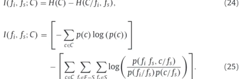
C/fi,fs)
, (24) I(
fi,fs;C)
= − c∈C p(
c)
log(
p(
c))
− c∈C fi∈F−S fs∈S log p(
fi fs,c/fs)
p(
fi/fs)
p(
c/fs)
. (25)The method uses the following iterative forward greedy search al-gorithm to find the relevant feature subset of sizekwithin the feature space:
Algorithm 1.Forward greedy search.
1. (Initialisation) SetF←“initial set ofnfeatures”;S←“empty set.” 2. (Computation of the MI with the output class) For∀fi ∈FcomputeI(C; fi). 3. (Choice of the first feature) Find a featurefithat maximisesI(C; fi); set
F ←F\{fi};setS←{fi}.
4. (Greedy selection) Repeat until|S|=k: (Selection of the next feature) Choose the featurefi=argmaxfi∈F−S(minfs∈S(I(fi,fs;C))); setF ←F\ {fi}; set S←S∪{fi}.
5. (Output) Output the setSwith the selected features.
5.2. Advantages over existing alternative methods
The Venn diagrams inFig. 1show different scenarios for the re-lationship between the candidate featurefi, the selected featurefs, and the class labelC.Fig. 1a illustrates the case in which methods like MIFS, NMIFS or mRMR will fail to selectfibecause it is redundant tofs, although each of them shares different information aboutC, and the correlation is not in the context ofC.
The goal function of JMIM is similar to the goal function of CMIM (Section 3), as CMIM also uses the ‘maximum of the mini-mum’ approach. The main difference is that CMIM maximises the amount of information the candidate featureficontributes given the pre-selected featurefs(i.e.fiis selected for any complementingfs), whereas JMIM selects the feature that maximises the joint mutual information withfs.Fig. 1b and c is used to explain this difference further. The figures represent two candidate featuresfiandfj, and the subsequent selection of one of them.I(fi, fs;C) is the union of areas 1, 2, and 3;I(fi;C/fs) is area 1 inFig. 1b. The CMIM method would se-lectfiinFig. 1b, even though its complementing featurefsfrom the subset does not carry as much information as the featurefjinFig. 1c. Conversely, JMIM would select the feature that maximises JMI, so it would select featurefiinFig. 1c. Therefore, the joint mutual infor-mation between the candidate feature and at least one of the pre-selected features will be high, which can increase the discrimination power of the selected subset.
5.3. Normalised Joint Mutual Information Maximisation (NJMIM)
The second method proposed in this paper uses a goal function, which is very similar to the one used in JMIM proposed inSection 5.1, with the difference being that symmetrical relevance is used as an alternative to MI. This method is called Normalised Joint Mutual Information Maximisation (NJMIM). It is proposed in order to study the effect of using normalised MI instead of MI. the proposed NJMIM selection criteria is presented inEq. (26).
FNJMIM=argmaxfi∈F−S
minfs∈S
(
SR(
fi,fs;C))
, (26)
where
Symmetrical rele
v
ance=SR(
F;C)
= I(
F;C)
H
(
F,C)
. (27)Which can be simplified as: FNJMIM=argmaxfi∈F−S
minfs∈S I(
fi,fs;C)
H(
fi,fs,C)
. (28)
The same iterative forward greedy search algorithm is used to find the subset of features within the candidate feature space.
6. Evaluation
The performance of the two proposed methods in this paper, JMIM and NJMIM, is compared with the results produced by five other methods: CMIM, DISR, mRMR, JMI, and IG. These methods are chosen for the following four reasons: (i) these methods are reported in the literature to provide good performance (Brown et al., 2012; Freeman et al., 2015); (ii) the choice of these methods allows the comparison of the ‘maximum of the minimum’ approach used by JMIM and NJMIM with the cumulative summation used by JMI and DISR; (iii) it enables the analysis of the effect of using the symmetrical relevance instead of MI on the algorithm’s performance; (iv) it allows the comparison of the effects of using joint mutual information and conditional mutual information, which are employed in JMIM and CMIM, respectively.
The seven methods are applied to data from different domains such as: life sciences, physical sciences, engineering, business, hand-writing recognition, and gene microarray. The features within these datasets have different characteristics, being binary, discrete or cate-gorical, or continuous. The continuous features are discretised into 10 equal intervals, using the Equal Width Discretisation (EWD) method (Dougherty, Kohavi, & Sahami, 1995).
Two classifiers are used to evaluate the quality of the selected sub-sets. These are Naïve-Bayes with kernel density estimation, and 3-Nearest Neighbours. Both classifiers are available in the Matlab Statis-tics Toolbox. The average classification accuracy is used as a measure of the quality of the selected features. Five-fold cross-validation is
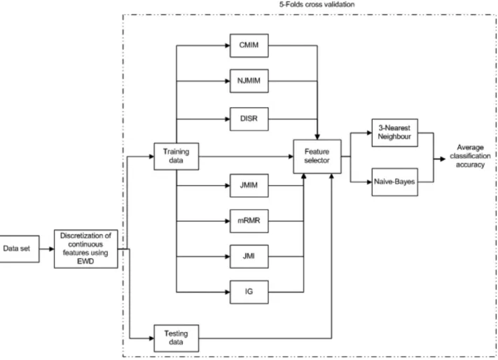
Fig. 2. Evaluation framework.
employed when processing feature selection and feature validation; therefore each fold is used for validation once. This means that 80% of the data is used for feature selection and classification training, whilst 20% is used for validation. This is repeated five times, using the whole dataset for validation over the course of five experiments. Overall, five different subsets of samples are used to generate five different sub-sets of features. Discretisation is performed as a pre-processing step for all data prior to the feature selection step.
Fig. 2shows the evaluation framework used in this experiment. To test the impact of adding each feature to the subset on the clas-sification accuracy, training and validation are performed after the selection of each feature in the subset.
6.1. Data
Eight datasets from the UCI Repository (Bache & Lichman, 2013) are used in the experiment (Table 1). These datasets have been pre-viously used in similar research (Brown et al., 2012; El Akadi et al., 2008; Cheng et al., 2011). They have different characteristics in terms of number of classes, features, instances and feature types.
An example-feature ratio (Brown et al., 2012) is used as an indica-tion of the difficulty of the feature selecindica-tion task for the dataset. This ratio is computed using N
mC, whereNis the number of instances,m is the median number of values that the features have, andCis the number of classes. The most challenging feature selection tasks are those performed using datasets with a small example-feature ratio. Thelibra movementdataset is the most challenging dataset.
To test the behaviour of the methods with an extremely small sample, datasets fromPeng et al. (2005)are also used in the evalu-ation process, and these are shown inTable 2.
Table 1
UCI datasets used in the experiment.
No Data set Number of Number of Number of Ratio features instances classes
1 Credit approval 15 690 2 54 2 Gas sensor 128 13874 6 198 3 Libra movement 90 483 15 3 4 Parkinson 22 195 2 11 5 Breast 30 569 2 28 6 Sonar 60 208 2 10 7 Musk 166 7074 2 354 8 Handwriting 649 2000 10 20 Table 2
Additional datasets used in the experiment (Peng et al., 2005).
No Data set Number of Number of Number of Ratio features instances classes
1 Colon 2000 62 2 10
2 Leukemia 7070 72 2 12
3 Lymphoma 4026 96 9 4
6.2. Performance analysis on low dimensional datasets
Figs. 3–5show the average classification accuracy of the three datasets with low numbers of features (Parkinson, credit approval and breast). The classification is computed over the whole size of the se-lected subset, from 1 feature up to 20 features (or all features of the dataset in the case of thecredit approvaldataset).
0 2 4 6 8 10 12 14 16 18 20 0.82 0.83 0.84 0.85 0.86 0.87 0.88 0.89 0.9 0.91 Classification accuracy CMIM NJMIM DISR JMIM mRMR JMI IG Number of features
Fig. 3.Average classification accuracy achieved with theParkinsondataset.
0 5 10 15 0.65 0.7 0.75 0.8 0.85 Number of features CMIM NJMIM DISR JMIM mRMR JMI IG C lass ifi c a tion ac c urac y
Fig. 4. Average classification accuracy achieved with thecredit approvaldataset.
0 2 4 6 8 10 12 14 16 18 20 0.82 0.84 0.86 0.88 0.9 0.92 0.94 0.96 0.98 1 Number of features C lassi fi ca tion a c cu ra cy CMIM NJMIM DISR JMIM mRMR JMI IG
As shown inFig. 3, which illustrates the experiment with the first dataset, JMIM achieves the highest average accuracy (90.77%) with just 8 features, which is higher than the accuracy of CMIM (90.26%) and JMI (88.97%). On the other hand, methods that use normalised MI, such as NJMIM and DISR, perform less well than JMIM and JMI, which use MI. This is expected for datasets with discrete features, because the normalisation may reduce the significance of the feature when it has high entropy and shares a high amount of information with the class label. The mRMR and IG methods perform poorly on this dataset. JMIM and JMI again achieve the highest classification accuracy on thecredit approvaldataset, using only 4 features to reach an accuracy of 82.92%. The accuracy of CMIM is 79.17% with the same number of features. The other methods perform worse compared to JMIM and JMI with the same number of features. The figure also shows that the methods using normalised MI do not perform as well as those which use MI. Features selected by the JMIM and JMI methods have a higher discriminative power than the features which are selected by NJMIM and DISR. NJMIM performs better than DISR, yet both perform poorly.
Thebreastdataset has 20 features selected. As seen inFig. 5, JMIM does not achieve the highest classification accuracy. However, it
produces a high accuracy (95.87%) with only 5 features, while mRMR requires 14 features to achieve the same accuracy. JMIM performs better in comparison with JMI and CMIM. The performance of NJMIM and DISR is not as good as JMIM and JMI, as with 4 features their classification accuracies are 87.61% and 89.28%, respectively.
6.3. Performance analysis on high dimensional datasets
The second experiment involves high dimensional data (musk, sonar, gas sensor, and handwritingdatasets. The experiment with the
gas sensorandsonardatasets includes the selection of 50 features, with JMIM achieving high classification accuracy with a relatively small number of features. The other methods require more features to achieve this level of accuracy (Figs. 6–7).
Fig. 8shows the results for thehandwritingdataset. 50 features are selected. JMIM performs well, but is inferior to JMI and mRMR. In terms of classification accuracy of the selected subset JMI per-formed better than JMIM in the subset with 11–21 features, by a maximum difference in accuracy of 0.5%. The mRMR method also performs well with this dataset; however JMIM produces the highest accuracy (97.68%) with the selected subset of 33 features.
0 5 10 15 20 25 30 35 40 45 50 0.2 0.3 0.4 0.5 0.6 0.7 0.8 0.9 Number of features Classi fi c a tion ac curac y CMIM NJMIM DISR JMIM mRMR JMI IG
Fig. 6. Average classification accuracy achieved with thegas sensordataset.
0 5 10 15 20 25 30 35 40 45 50 0.65 0.7 0.75 0.8 0.85 Number of features CMIM NJMIM DISR JMIM mRMR JMI IG Classification accuracy
0 10 20 30 40 50 60 70 80 90 100 0.4 0.5 0.6 0.7 0.8 0.9 1 Number of features y c ar u c c a n oit a cif i s s al C CMIM NJMIM DISR FIM JMIM mRMR JMI IG 32 34 36 38 40 42 44 0.9 0.91 0.92 0.93 0.94 0.95 0.96 0.97 0.98
Fig. 8.Average classification accuracy achieved with thehandwritingdataset.
0 5 10 15 20 25 30 35 40 45 50 0.2 0.3 0.4 0.5 0.6 0.7 0.8 0.9 1 Number of features Classification accuracy CMIM NJMIM DISR FIM JMIM mRMR JMI IG 14 16 18 20 22 24 0.65 0.7 0.75 0.8
Fig. 9.Average classification accuracy achieved with thelibra movementdataset.
The experimental results using the libra movementdataset are shown in Fig. 9, when 50 features are selected. JMIM is the best method with this dataset with almost any number of selected fea-tures, followed by NJMIM. JMIM outperforms JMI by up to 3% in terms of classification accuracy. NJMIM also outperforms DISR for all of the selected subsets.
The methods are also applied to themuskdataset.Fig. 10shows the result when 50 features are selected. With this dataset, JMIM se-lects the best subset and outperforms the other methods in terms of classification accuracy. NJMIM does not perform as well as JMIM, but produces better accuracy than DISR and mRMR for most of the fea-tures selected.
6.4. Performance analysis withPeng et al. (2005)datasets
The results using the three datasets employed byPeng et al. (2005) are shown inFig. 11. The leukemia dataset (Fig. 11a) has a small num-ber of samples. The results show that none of the feature selection
methods perform particularly well, confirming the findings reported in the review article byBrown et al. (2012). Thecolondataset, which is the least challenging dataset of the three in terms of the number of classes and features, is shown inFig. 11b. The results indicate the better performance of JMIM and JMI compared to the other meth-ods, especially CMIM, which performs poorly. However, CMIM is the method that provides the best accuracy with thelymphomadataset, while JMIM, JMI and mRMR also perform well, with JMIM being the best of these. NJMIM performs better than DISR with all of the subsets below 34 features.
6.5. Evaluating and validating results
ANOVA statistical test is employed to analyse the results, and to confirm that the results are systematic and they were not ob-tained by chance. The classification experiment is run five times for each dataset and the average accuracy results are submitted to the ANOVA test.Table 3shows the ANOVA results, whereP-value is the
0 5 10 15 20 25 30 35 40 45 50 0.55 0.6 0.65 0.7 0.75 0.8 0.85 0.9 0.95 Number of features C lassification accuracy CMIM NJMIM DISR JMIM mRMR JMI IG
Fig. 10. Average classification accuracy achieved with themuskdataset.
Table 3
ANOVA test.
Dataset MS F P-value
Credit approval 0.027537 731.3342 1.87E−37 Gas sensor 0.004117 77.17653 1.38E−16 Libra movement 0.009677 114.5907 2.94E−23 Parkinson 0.009677 114.5907 2.94E−23
Breast 0.001414 101.4627 2.37E−22
Sonar 0.00094 5.760126 9.62E−05
Musk 0.000505 304.4366 1.11E−30
Handwriting 8.84E−05 35.99929 6.35E−15
Colon 0.000411 3.532383 0.006395
Leukemia 0.000161 10.36207 2.21E−07 Lymphoma 0.011501 232.6585 1.28E−28
probability of the improvement to occur by chance, and MS is the mean square error. When the value of theP-value is less than 0.05 it is unlikely that the improvement in classification accuracy happened by chance. This is shown to be the case for all the datasets (Table 3).
6.6. Stability of the methods
This section focuses on the stability of the feature selection meth-ods discussed. The selected subset features are dependent on the datasets provided, and therefore any change to the data might lead to different selected features. In this context, the present study investigates the influence of changes in the data on the features selected.
Kuncheva’s measure of stability (Kuncheva, 2007), known as the consistency index, usesEq. (29)to compute the consistency between two selected feature subsets,S1andS2:
S1,S2
= rn−k2k
(
n−k)
, (29)whereS1andS2are selected feature subsets using different groups of
dataset samples, i.e.S1,S2∈FwhereFis the total set of the feature,
|
S1|
=|
S2|
=k,|
F|
=n, andr=|
S1∩S2|
. However, this method doesnot take into consideration the correlation between features.
Yu, Ding, and Loscalzo (2008)proposed a method for measuring
stability based on similarity. This method takes into account the cor-relation between features. It calculates the weight between each pair of features from the subsetsS1andS2, computes the similarity
be-tweenS1andS2, and constructs a bipartite graph. Iff
iis a feature
be-Table 4
Average stability, average accuracy and the compromise between accuracy and stability.
Method Accuracy Stability Accuracy/stability CIMIM 0.8488 0.8598 0.9197 NJMIM 0.8264 0.8344 0.8954 DISR 0.8129 0.9054 0.8807 JMIM 0.8578 0.8598 0.9294 mRMR 0.8278 0.8868 0.8969 JMI 0.8490 0.8838 0.9199 IG 0.8226 0.9228 0.8913 longing toS1andf
jis a feature belonging toS2, the value of the weight can be the correlation coefficient, or any other similarity measure.
This article uses symmetrical uncertainty (Yu & Liu, 2004) to cal-culate the weightw:
w
s1i,s2j=2 Is1 i,s 2 j Hs1 i +Hs2 j , (30) where 0≤w(
s1 i,s 2j
)
≤1.0. To find the maximum weighted bipartite matching, the Hungarian Algorithm (Kuhn, 1955) is used to find the optimal solution.This experiment uses the eight UCI datasets, as shown inTable 1. Each dataset is divided into 5 folds, 4 of which are used for feature selection using the CMIM, NJMIM, DISR, JMIM, mRMR, JMI, and IG methods.Eq. (30)is used to calculate the weight between the features within each pair of selected subsets from each dataset. The final cost is divided over the cardinality of the subset used, and therefore the magnitude of the final cost should be less than or equal to 0.5 (it is 0.5 if all selected subsets are the same).
The relationship between accuracy and stability is computed by comparing the average classification accuracy and the average stabil-ity with different numbers of features.
Table 4shows the average accuracy/stability for each method in no particular order. It is worth noting that the methods employing the ‘maximum of the minimum’ criterion (JMIM, NJMIM and CMIM) tend to have lower stability than the methods using the cumulative summation approximation (JMI and DISR). The best method in terms of stability is IG. JMIM has the best compromise between accuracy and stability. Moreover, it demonstrates the best average classifica-tion accuracy among all methods.
a-
Leukemia
0 5 10 15 20 25 30 35 40 45 50 0.84 0.86 0.88 0.9 0.92 0.94 0.96 0.98 1 Number of features Classification accuracy CMIM NJMIM DISR FIM JMIM mRMR JMI IGb-Colon
0 5 10 15 20 25 30 35 40 45 50 0.74 0.76 0.78 0.8 0.82 0.84 0.86 Number of features Classification accuracyc-Lymphoma
0 10 20 30 40 50 60 0.5 0.55 0.6 0.65 0.7 0.75 0.8 0.85 0.9 0.95 Number of features Classification accuracy7. Discussion
The JMIM method outperforms the other methods when tested with most of the datasets in terms of selecting the subset that pro-duces the best classification accuracy. JMIM also propro-duces the best accuracy with the datasets with a low number of features, such as the
Parkinson, credit approval and breastdatasets. In these experiments, the maximum average classification accuracy achieved by JMIM with theParkinsondataset was 90.77%. JMIM and JMI achieved the accu-racy of 82.92% with thecredit approvaldataset whilst JMI and CMIM achieved 93.83% and 95.22%, respectively. The JMIM method also per-formed well on high dimensional datasets, such as themusk, sonar, gas sensor and handwritingdatasets.
JMIM and JMI also outperform the other methods on extremely small sample datasets with a large number of features, such as the
colondataset. However, CMIM produces the best performance with thelymphomadataset. JMIM, JMI, and mRMR also perform better than the other three methods. Overall, JMIM decreases the average classi-fication error by 0.88% in absolute terms and almost 6% in relative terms in comparison to the next best performing method, JMI. The JMIM classification accuracy is also higher than that reported in lit-erature by other filter methods (Zhang et al., 2015), although no firm conclusions can be made on this account due to the variety of the datasets used in the most recent articles (Liang et al., 2014; Zhang et al., 2015).
In addition to the quantitative assessment of the accuracy of the proposed methods, several experiments are conducted to enable an in-depth comparison of different feature selection methods, accord-ing to several criteria. For example, the nonlinear approach, which uses the ‘maximum of the minimum’ criterion, is compared to the linear approach that employs cumulative summation approximation. In particular, JMIM is compared to JMI, with the results showing that the non-linear approach performed better than the linear approach when tested with most of the datasets.
The goal function based on joint mutual information is compared to the goal function based on conditional mutual information, with the result showing better performance of joint mutual information in combination with the non-linear criterion.
Finally, the effect of using normalised mutual information instead of mutual information is tested by comparing the performance of JMIM and JMI with NJMIM and DISR. The results show that, with the discretised datasets, the methods employing non normalised mutual information such as JMI and JMIM perform better than those using normalised mutual information, such as DISR and NJMIM. This sug-gests that division of the mutual information over the joint entropy does not improve performance.
In addition, the methods are compared in terms of their stability, as described in detail inSection 6.5. The results demonstrate that the methods employing ‘maximum of the minimum’ criterion, such as CMIM, JMIM, and NJMIM, show less average stability than the meth-ods which employ cumulative summation, although there is no dom-inant method.
8. Conclusion
This paper presents two new feature selection methods based on information theory: Joint Mutual Information Maximisation (JMIM) and Normalised Joint Mutual Information Maximisation (NJMIM). These methods are designed to resolve the problem of choosing redundant and irrelevant features in certain circumstances, which is characteristic of filter feature selection methods. The latter is achieved through the use of the mutual information and the ‘max-imum of the min‘max-imum’ nonlinear approach for the goal function design.
The methods have been evaluated using public datasets and com-pared with five other feature selection methods: Joint Mutual
Infor-mation (JMI), Conditional Mutual InforInfor-mation Maximisation (CMIM), Maximum Relevancy Minimum Redundancy (mRMR), Double Input Symmetrical Relevance (DISR), and Information Gain (IG) in terms of their ability to select features with high discriminative power, and their stability. To evaluate the performance of the proposed methods, an experiment is conducted using eight datasets from the UCI Reposi-tory. In addition, to test the behaviour of the methods with extremely small sample datasets, three other datasets fromPeng et al. (2005) are used.
Overall, JMIM decreases the average classification error by 0.88% in absolute terms and almost by 6% in relative terms in comparison to the next best performing method, JMI. The statistical significance of the reported results is further confirmed by ANOVA test. Moreover, this method produces the best trade-off between accuracy and stabil-ity. The limitations of our approach are those which are characteristic of other filter approaches: it disregards the interaction between the features and the classifier, as well as the higher dimensional joint mu-tual information between more than two features, which sometimes can lead to suboptimal choice of features.
Future work includes more experiments using other search strate-gies to validate the proposed method in a wider range of search algorithms, employing parallel computation techniques to estimate higher dimensional joint mutual information in which two or more of the features from the selected subset are used simultaneously to test the significance of the candidate feature, automating the selection of the optimal subset by introducing a cut-off parameter measuring the relevancy of the features.
Further improvements can be made by studying the information shared between features and class labels and classifying the fea-tures into strongly relevant, relevant, weakly relevant, and redundant based on the information that the feature adds to the selected subset. In terms of applications relevant to expert and intelligent systems, JMIM method would be of benefit for choosing the most relevant fea-tures in classification tasks. In addition to the analysis of the public datasets in this article, the method could be used in many other ap-plications where the relevance of the features for the classification task needs to be analysed.
References
Bache, K., & Lichman, M. (2013).UCI machine learning repository. Irvine, CA: Univer-sity of California, School of Information and Computer Science. (http://archive. ics.uci.edu/ml).
Bajwa, I., Naweed, M., Asif, M., & Hyder, S. (2009). Feature based image classification by using principal component analysis.ICGST International Journal on Graphics Vision and Image Processing, 9, 11–17.
Battiti, R. (1994). Using mutual information for selecting features in supervised neural net learning.IEEE Transactions on Neural Networks, 5, 537–550.
Bolón-Canedo, V., Sánchez-Maroño, N., & Alonso-Betanzos, A. (2013). A review of fea-ture selection methods on synthetic data.Knowledge and Information Systems, 34, 483–519.
Brown, G., Pocock, A., Zhao, M., & Lujan, M. (2012). Conditional likelihood maximisa-tion: a unifying framework for information theoretic feature selection.Journal of Machine Learning Research, 13, 27–66.
Chandrashekar, G., & Sahin, F. (2014). A survey on feature selection methods.Computers and Electrical Engineering, 40, 16–28.
Cheng, H., Qin, Z., Feng, C., Wang, Y., & Li, F. (2011). Conditional mutual information-based feature selection analysing for synergy and redundancy.Electronics and Telecommunications Research Institute, 33, 210–218.
Cover, T., & Thomas, J. (2006).Elements of information theory. New York: John Wiley & Sons.
Ding, C., & Peng, H. (2003). Minimum redundancy feature selection from microarray gene expression data. InProceedings of the computational systems bioinformatics: IEEE Computer Society(pp. 523–528).
Dougherty, J., Kohavi, R., & Sahami, M. (1995). Supervised and unsupervised discretiza-tion of continuous features. InProceedings of the twelfth international conference on machine learning(pp. 194–202).
Duda, R., Hart, P., & Stork, D. (2001).Pattern classification. New York: John Wiley and Sons.
El Akadi, A., El Ouardighi, A., & Aboutajdine, D. (2008). A powerful feature selection approach based on mutual information.International Journal of Computer Science and Network Security, 8, 116–121.
Estévez, P. A., Tesmer, M., Perez, A., & Zurada, J. M. (2009). Normalized mutual informa-tion feature selecinforma-tion.IEEE Transactions on Neural Networks, 20, 189–201.
Fleuret, F. (2004). Fast binary feature selection with conditional mutual information. Journal of Machine Learning Research, 5, 1531–1555.
Freeman, C., Kuli ´c, D., & Basir, O. (2015). An evaluation of classifier-specific filter mea-sure performance for feature selection.Pattern Recognition, 48, 1812–1826. Guyon, I., & Elisseeff, A. (2003). An introduction to variable and feature selection.
Jour-nal of Machine Learning Research, 3, 1157–1182.
Guyon, I., Gunn, S., Nikravesh, M., & Zadeh, L. A. (2006).Feature extraction foundations and applications. New York/Berlin, Heidelberg: Springer Studies in fuzziness and soft computing.
Hoque, N., Bhattacharyya, D. K., & Kalita, J. K. (2014). MIFS-ND: a mutual information-based feature selection method.Expert Systems with Applications, 41(14), 6371– 6385.
Jain, A. K., Duin, R. P. W., & Mao, J. (2000). Statistical Pattern Recognition: A Review. IEEE Transactions on Pattern Analysis and Machine Intelligence, 22, 4–37.
Jakulin, A. (2003).Attribute interactions in machine learning. (M.S.c thesis), Computer and Information Science, University of Ljubljana.
Jakulin, A. (2005).Machine learning based on attribute interactions (Ph.D. thesis), Com-puter and Information Science, University of Ljubljana.
Janecek, A., Gansterer, W., Demel, M., & Ecker, G. (2008). On the relationship between feature selection and classification accuracy.Journal of Machine Learning Research: Workshop and Conference Proceedings, 4, 90–105.
Karegowda, A. G., Jayaram, M. A., & Manjunath, A. S. (2010). Feature subset selection problem using wrapper approach in supervised learning.International Journal of Computer Applications, 1, 13–17.
Kira, K., & Rendell, L. (1992). A practical approach to feature selection. InProceedings of the 10th International Workshop on Machine Learning (ML92)(pp. 249–256). Kuhn, H. (1955). The Hungarian method for the assignment problem.Naval Research
Logistic Quarterly, 2, 83–97.
Kuncheva, L. (2007). A stability index for feature selection. InProceedings of the 25th IASTED International Multi-Conference on Artificial Intelligence and Applications (pp. 390–395).
Kwok, N., & Choi, C. (2002). Input feature selection for classification problems.IEEE Transactions on Neural Networks, 13, 143–159.
Lee, J., & Kim, D. (2015). Fast multi-label feature selection based on information-theoretic feature ranking.Pattern Recognition, 48, 2761–2771.
Liang, J., Wang, F., Dang, C., & Qian, Y. (2014). A group incremental approach to feature selection applying rough set technique.IEEE Transactions on Knowledge and Data Engineering, 26(2), 294–308.
Lin, T., Li, H., & Tsai, K. (2004). Implementing the fisher’s discriminant ratio in a k-means clustering algorithm for feature selection and dataset trimming.Journal of Chemical Information and Computer Sciences, 44, 76–87.
Liu, H., & Motoda, H. (2008).Computational methods of feature selection. New York: Chapman & Hall/CRC Taylor & Francis Group.
Liu, H., & Yu, L. (2005). Toward integrating feature selection algorithms for classification and clustering.IEEE Transactions on Knowledge and Data Engineering, 17, 491–502.
Meyer, P. E., & Bontempi, G. (2006). On the use of variable complementarity for feature selection in cancer classification. InProceedings of European workshop on applica-tions of evolutionary computing: Evo Workshops(pp. 91–102).
Meyer, P. E., Schretter, C., & Bontempi, G. (2008). Information-theoretic feature selec-tion in microarray data using variable complementarity.IEEE Journal of Selected Topics in Signal Processing, 2, 261–274.
Peng, H., Long, F., & Ding, C. (2005). Feature selection based on mutual information: cri-teria of max-dependency, max-relevance, and min-redundancy.IEEE Transactions on Pattern Analysis and Machine Intelligence, 27, 1226–1238.
Rodgers, J., & Nicewander, W. A. (1988). Thirteen ways to look at the correlation coeffi-cient.The American Statistician, 42, 59–66.
Qian, Y., Wang, Q., Cheng, H., Liang, J., & Dang, C. (2015). Fuzzy-rough feature selection accelerator.Fuzzy Sets and Systems, 258, 61–78.
Saeys, Y., Inza, I., & Larranaga, P. (2007). A review of feature selection techniques in bioinformatics.Bioinformatics, 23, 2507–2517.
Tang, E. K., Suganthana, P. N., Yao, X., & Qina, A. K. (2005). Linear dimensionality reduc-tion using relevance weighted LDA.Pattern Recognition, 38, 485–493.
Turk, M., & Pentland, A. (1991). Eigenfaces for recognition.Journal of Cognitive Neuro-science, 3, 72–86.
Vergara, J., & Estévez, P. (2014). A review of feature selection methods based on mutual information.Neural Computing and Applications, 24, 175–186.
Vidal-Naquet, M., & Ullman, S. (2003). Object recognition with informative features and linear classification. InProceedings of the 10th IEEE international conference on computer vision(pp. 281–289).
Yang, H., & Moody, J. (1999). Feature selection based on joint mutual information. In Proceedings of international ICSC symposium on advances in intelligent data analysis (pp. 22–25).
Yu, H., & Yang, J. (2001). A direct LDA algorithm for high-dimensional data with appli-cation to face recognition.Pattern Recognition, 34, 2067–2070.
Yu, L., & Liu, H. (2004). Efficient feature selection via analysis of relevance and redun-dancy.Journal of Machine Learning Research, 5, 1205–1224.
Yu, L., Ding, C., & Loscalzo, S. (2008). Stable feature selection via dense feature groups. InProceedings of the 14th ACM SIGKDD international conference on knowledge dis-covery and data mining(pp. 803–811).
Zhang, Y., Yang, A., Xiong, C., Wang, T., & Zhang, Z. (2014). Feature selection using data envelopment analysis.Knowledge-Based Systems, 64, 70–80.
Zhang, Y., Yang, C., Yang, A., Xiong, C. Y., Zhou, X., & Zhang, Z. (2015). Feature selection for classification with class-separability strategy and data envelopment analysis. Neurocomputing, 166, 172–184.