Edinburgh Research Explorer
Stochastic Dual Coordinate Ascent with Adaptive Probabilities
Citation for published version:
Csiba, D, Qu, Z & Richtárik, P 2015, 'Stochastic Dual Coordinate Ascent with Adaptive Probabilities' Paper presented at 32nd international conference on machine learning, Lille, France, 6/07/15 - 11/07/15, .
Link:
Link to publication record in Edinburgh Research Explorer
Document Version:
Early version, also known as pre-print
General rights
Copyright for the publications made accessible via the Edinburgh Research Explorer is retained by the author(s) and / or other copyright owners and it is a condition of accessing these publications that users recognise and abide by the legal requirements associated with these rights.
Take down policy
The University of Edinburgh has made every reasonable effort to ensure that Edinburgh Research Explorer content complies with UK legislation. If you believe that the public display of this file breaches copyright please contact [email protected] providing details, and we will remove access to the work immediately and investigate your claim.
arXiv:1502.08053v1 [math.OC] 27 Feb 2015
Stochastic Dual Coordinate Ascent with Adaptive Probabilities
Dominik Csiba [email protected]
Zheng Qu [email protected]
Peter Richt´arik [email protected]
University of Edinburgh
Abstract
This paper introduces AdaSDCA: an adap-tive variant of stochastic dual coordinate as-cent (SDCA) for solving the regularized empir-ical risk minimization problems. Our modifica-tion consists in allowing the method adaptively change the probability distribution over the dual variables throughout the iterative process. AdaS-DCA achieves provably better complexity bound than SDCA with the best fixed probability dis-tribution, known as importance sampling. How-ever, it is of a theoretical character as it is expen-sive to implement. We also propose AdaSDCA+: a practical variant which in our experiments out-performs existing non-adaptive methods.
1. Introduction
Empirical Loss Minimization. In this paper we consider
the regularized empirical risk minimization problem:
min w∈Rd " P(w)def= 1 n n X i=1 φi(A⊤i w) +λg(w) # . (1)
In the context of supervised learning,wis a linear predictor,
A1, . . . , An ∈ Rd are samples,φ1, . . . , φn : Rd → Rare
loss functions,g : Rd → Ris a regularizer and λ >0 a
regularization parameter. Hence, we are seeking to identify the predictor which minimizes the average (empirical) loss
P(w).
We assume throughout that the loss functions are 1/γ -smooth for some γ > 0. That is, we assume they are differentiable and have Lipschitz derivative with Lipschitz constant1/γ:
|φ′(a)−φ′(b)| ≤ γ1|a−b|
for alla, b∈R. Moreover, we assume thatgis1-strongly convex with respect to the L2 norm:
g(w)≤αg(w1) + (1−α)g(w2)−
α(1−α)
2 kw1−w2k 2
for allw1, w2 ∈domg,0≤α≤1andw=αw1+ (1−
α)w2.
The ERM problem (1) has received considerable attention in recent years due to its widespread usage in supervised statistical learning (Shalev-Shwartz & Zhang,2013b). Of-ten, the number of samples nis very large and it is im-portant to design algorithms that would be efficient in this regime.
Modern stochastic algorithms for ERM. Several highly efficient methods for solving the ERM prob-lem were proposed and analyzed recently. These include primal methods such as SAG (Schmidt et al.,
2013), SVRG (Johnson & Zhang, 2013), S2GD (Koneˇcn ´y & Richt´arik, 2014), SAGA (Defazio et al.,
2014), mS2GD (Koneˇcn ´y et al.,2014a) and MISO (Mairal,
2014). Importance sampling was considered in ProxSVRG (Xiao & Zhang,2014) and S2CD (Koneˇcn ´y et al.,2014b).
Stochastic Dual Coordinate Ascent. One of the most
suc-cessful methods in this category is stochastic dual
coor-dinate ascent (SDCA), which operates on the dual of the
ERM problem (1):
max
α=(α1,...,αn)∈Rn
h
D(α)def=−f(α)−ψ(α)i, (2)
where functionsfandψare defined by
f(α)def=λg∗ 1 λn n X i=1 Aiαi ! , (3) ψ(α)def= 1 n n X i=1 φ∗ i(−αi), (4) andg∗andφ∗
i are the convex conjugates1ofgandφi,
re-spectively. Note that in dual problem, there are as many variables as there are samples in the primal:α∈Rn.
SDCA in each iteration randomly selects a dual variable
αi, and performs its update, usually via closed-form 1
By the convex (Fenchel) conjugate of a function h : Rk
→ R we mean the functionh∗ : Rk
→ Rdefined by
formula – this strategy is know as randomized coor-dinate descent. Methods based on updating randomly selected dual variables enjoy, in our setting, a linear convergence rate (Shalev-Shwartz & Zhang,2013b;2012;
Tak´aˇc et al., 2013; Shalev-Shwartz & Zhang, 2013a;
Zhao & Zhang, 2014; Qu et al., 2014). These methods have attracted considerable attention in the past few years, and include SCD (Shalev-Shwartz & Tewari,2011), RCDM (Nesterov, 2012), UCDC (Richt´arik & Tak´aˇc,
2014), ICD (Tappenden et al., 2013), PCDM (Richt´arik & Tak´aˇc, 2012), SPCDM (Fercoq & Richt´arik,
2013), SPDC (Zhang & Xiao, 2014), APCG (Lin et al.,
2014), RCD (Necoara & Patrascu, 2014), APPROX (Fercoq & Richt´arik, 2013), QUARTZ (Qu et al.,
2014) and ALPHA (Qu & Richt´arik, 2014). Re-cent advances on mini-batch and distributed variants can be found in (Liu & Wright, 2014), (Zhao et al.,
2014b), (Richt´arik & Tak´aˇc, 2013a), (Fercoq et al.,
2014), (Trofimov & Genkin, 2014), (Jaggi et al., 2014), (Mareˇcek et al., 2014) and (Mahajan et al., 2014). Other related work includes (Nemirovski et al., 2009;
Duchi et al., 2011; Agarwal & Bottou, 2014; Zhao et al.,
2014a;Fountoulakis & Tappenden,2014;Tappenden et al.,
2014). We also point to (Wright, 2014) for a review on coordinate descent algorithms.
Selection Probabilities. Naturally, both the theoretical convergence rate and practical performance of random-ized coordinate descent methods depends on the proba-bility distribution governing the choice of individual co-ordinates. While most existing work assumes uniform distribution, it was shown by Richt´arik & Tak´aˇc (2014);
Necoara et al. (2012); Zhao & Zhang (2014) that coordi-nate descent works for an arbitrary fixed probability dis-tribution over individual coordinates and even subsets of coordinates (Richt´arik & Tak´aˇc, 2013b; Qu et al., 2014;
Qu & Richt´arik, 2014; Qu & Richt´arik, 2014). In all of these works the theory allows the computation of a fixed probability distribution, known as importance sampling, which optimizes the complexity bounds. However, such a distribution often depends on unknown quantities, such as the distances of the individual variables from their optimal values (Richt´arik & Tak´aˇc,2014;Qu & Richt´arik,
2014). In some cases, such as for smooth strongly con-vex functions or in the primal-dual setup we consider here, the probabilities forming an importance sampling can be explicitly computed (Richt´arik & Tak´aˇc, 2013b;
Zhao & Zhang, 2014; Qu et al., 2014; Qu & Richt´arik,
2014;Qu & Richt´arik,2014). Typically, the theoretical in-fluence of using the importance sampling is in the replace-ment of the maximum of certain data-dependent quantities in the complexity bound by the average.
Adaptivity. Despite the striking developments in the field,
there is virtually no literature on methods using an
adap-tive choice of the probabilities. We are aware of a few
pieces of work; but all resort to heuristics unsupported by theory (Glasmachers & Dogan, 2013; Lukasewitz, 2013;
Schaul et al.,2013;Banks-Watson,2012;Loshchilov et al.,
2011), which unfortunately also means that the methods are sometimes effective, and sometimes not. We observe
that in the primal-dual framework we consider, each dual variable can be equipped with a natural measure of progress which we call “dual residue”. We propose that the selection probabilities be constructed based on these quantities.
Outline: In Section2 we summarize the contributions of
our work. In Section3 we describe our first, theoretical methods (Algorithm1) and describe the intuition behind it. In Section4we provide convergence analysis. In Sec-tion5we introduce Algorithm2: an variant of Algorithm1
containing heuristic elements which make it efficiently im-plementable. We conclude with numerical experiments in Section6. Technical proofs and additional numerical ex-periments can be found in the appendix.
2. Contributions
We now briefly highlight the main contributions of this work.
Two algorithms with adaptive probabilities. We propose
two new stochastic dual ascent algorithms: AdaSDCA (Al-gorithm1) and AdaSDCA+ (Algorithm2) for solving (1) and its dual problem (2). The novelty of our algorithms is in adaptive choice of the probability distribution over the dual coordinates.
Complexity analysis. We provide a convergence rate
anal-ysis for the first method, showing that AdaSDCA enjoys
better rate than the best known rate for SDCA with a fixed sampling (Zhao & Zhang,2014;Qu et al.,2014). The probabilities are proportional to a certain measure of dual suboptimality associated with each variable.
Practical method. AdaSDCA requires the same com-putational effort per iteration as the batch gradient algo-rithm. To solve this issue, we propose AdaSDCA+ (Algo-rithm2): an efficient heuristic variant of the AdaSDCA. The computational effort of the heuristic method in a sin-gle iteration is low, which makes it very competitive with methods based on importance sampling, such as IProx-SDCA (Zhao & Zhang,2014). We support this with com-putational experiments in Section6.
Outline: In Section2 we summarize the contributions of
our work. In Section3 we describe our first, theoretical methods (AdaSDCA) and describe the intuition behind it. In Section 4 we provide convergence analysis. In Sec-tion 5we introduce AdaSDCA+: a variant of AdaSDCA
containing heuristic elements which make it efficiently im-plementable. We conclude with numerical experiments in Section6. Technical proofs and additional numerical ex-periments can be found in the appendix.
3. The Algorithm: AdaSDCA
It is well known that the optimal primal-dual pair
(w∗, α∗)∈Rd×Rnsatisfies the following optimality
con-ditions: w∗=∇g∗ 1 λnAα ∗ (5) α∗i =−∇φi(Ai⊤w∗), ∀i∈[n] def ={1, . . . , n}, (6) whereAis thed-by-nmatrix with columnsA1, . . . , An.
Definition 1 (Dual residue). The dual residue, κ = (κ1, . . . , κn)∈Rn, associated with(w, α)is given by:
κi
def
=αi+∇φi(A⊤i w). (7)
Note, thatκt
i = 0if and only ifαisatisfies (5). This
mo-tivates the design of AdaSDCA (Algorithm1) as follows: whenever|κt
i|is large, theith dual coordinateαiis
subop-timal and hence should be updated more often.
Definition 2 (Coherence). We say that probability vector
pt∈Rn is coherent with the dual residueκtif for alli∈
[n]we have
κt
i6= 0 ⇒ p t i >0.
Alternatively,ptis coherent withktif for
It def ={i∈[n] :κt i 6= 0} ⊆[n]. we havemini∈Itp t i>0.
AdaSDCA is a stochastic dual coordinate ascent method, with an adaptive probability vector pt, which could
po-tentially change at every iteration t. The primal and dual update rules are exactly the same as in standard SDCA (Shalev-Shwartz & Zhang, 2013b), which instead uses uniform sampling probability at every iteration and does not require the computation of the dual residueκ. Our first result highlights a key technical tool which ul-timately leads to the development of good adaptive sam-pling distributionsptin AdaSDCA. For simplicity we
de-note byEtthe expectation with respect to the random index
it∈[n]generated at iterationt.
Lemma 3. Consider the AdaSDCA algorithm during
iter-ationt≥0and assume thatptis coherent withκt. Then
Et D(αt+1)−D(αt) −θ P(wt)−D(αt) ≥ −2λnθ 2 X i∈It θ(v i+nλγ) pt i −nλγ |κti|2, (8) Algorithm 1 AdaSDCA
Init:vi=A⊤i Aifori∈[n];α0∈Rn;α¯0= λn1 Aα0
fort≥0do
Primal update:wt=∇g∗(¯αt)
Set:αt+1=αt
Compute residueκt:κt
i =αti+∇φi(A⊤i wt),∀i∈[n]
Compute probability distributionptcoherent withκt
Generate randomit∈[n]according topt
Compute: ∆αt it = arg max ∆∈R −φ∗it(−(α t it+ ∆)) −A⊤ itw t∆ − vit 2λn|∆| 2 Dual update:αti+1t =α t it+ ∆α t it Average update:α¯t= ¯αt+∆αit λn Ait end for Output:wt, αt for arbitrary 0≤θ≤min i∈It pt i. (9)
Proof. Lemma 3 is proved similarly to Lemma 2
in (Zhao & Zhang,2014), but in a slightly more general setting. For completeness, we provide the proof in the ap-pendix.
Lemma 3 plays a key role in the analysis of stochas-tic dual coordinate methods (Shalev-Shwartz & Zhang,
2013b; Zhao & Zhang, 2014; Shalev-Shwartz & Zhang,
2013a). Indeed, if the right-hand side of (8) is positive, then the primal dual errorP(wt)
−D(αt)can be bounded by
the expected dual ascentEt[D(αt+1)−D(αt)]times1/θ,
which yields the contraction of the dual error at the rate of
1−θ (see Theorem7). In order to make the right-hand side of (8) positive we can take anyθsmaller thanθ(κt, pt)
where the functionθ(·,·) :Rn
+×Rn+→Ris defined by: θ(κ, p)≡ nλγ P i:κi6=0|κi| 2 P i:κi6=0p −1 i |κi|2(vi+nλγ) . (10)
We also need to make sure that0 ≤ θ ≤ mini∈Itp
t i in
order to apply Lemma3. A “good” adaptive probabilitypt
should then be the solution of the following optimization problem: max p∈Rn + θ(κt, p) (11) s.t. n X i=1 pi= 1 θ(κt, p) ≤ min i:κt i6=0 pi
A feasible solution to (11) is the importance sampling (also known as optimal serial sampling)p∗defined by:
p∗ i def = Pnvi+nλγ j=1(vj+nλγ) , ∀i∈[n], (12)
which was proposed in (Zhao & Zhang, 2014) to obtain proximal stochastic dual coordinate ascent method with importance sampling (IProx-SDCA). The same optimal probability vector was also deduced, via different means and in a more general setting in (Qu et al.,2014). Note that in this special case, sinceptis independent of the residue
κt, the computation of κt is unnecessary and hence the
complexity of each iteration does not scale up withn. It seems difficult to identify other feasible solutions to program (11) apart from p∗, not to mention solve it
ex-actly. However, by relaxing the constraint θ(κt, p) ≤
mini:κt
i6=0pi, we obtain an explicit optimal solution. Lemma 4. The optimal solutionp∗(κt)of
max p∈Rn + θ(κt, p) (13) s.t. n X i=1 pi= 1 is: (p∗(κt)) i= | κt i| √ vi+nλγ Pn j=1|κtj| p vj+nλγ , ∀i∈[n]. (14)
Proof. The proof is deferred to the appendix.
The suggestion made by (14) is clear: we should update more often those dual coordinatesαiwhich have large
ab-solute dual residue|κt
i|and/or large Lipschitz constantvi.
If we letpt =p∗(κt)andθ=θ(κt, pt), the constraint (9)
may not be sastified, in which case (8) does not neces-sarily hold. However, as shown by the next lemma, the constraint (9) is not required for obtaining (8) when all the functions{φi}iare quadratic.
Lemma 5. Suppose that all{φi}iare quadratic. Lett≥0.
Ifmini∈Itp
t
i >0, then (8) holds for anyθ∈[0,+∞).
The proof is deferred to Appendix.
4. Convergence results
In this section we present our theoretical complexity results for AdaSDCA. The main results are formulated in Theo-rem7, covering the general case, and in Theorem11in the special case when{φi}ni=1are all quadratic.
4.1. General loss functions
We derive the convergence result from Lemma3.
Proposition 6. Let t ≥ 0. If mini∈Itp
t i > 0 and θ(κt, pt) ≤mini∈Itp t i, then Et D(αt+1)−D(αt) ≥θ(κt, pt) P(wt)−D(αt) .
Proof. This follows directly from Lemma 3 and the fact
that the right-hand side of (8) equals 0 whenθ=θ(κt, pt).
Theorem 7. Consider AdaSDCA. If at each iterationt≥ 0,mini∈Itp t i >0andθ(κt, pt)≤mini∈Itp t i, then E[P(wt)−D(αt)]≤ ˜1 θt t Y k=0 (1−θ˜k) D(α∗)−D(α0) , (15)
for allt≥0where
˜ θt def = E[θ(κ t, pt)(P(wt) −D(αt))] E[P(wt)−D(αt)] . (16)
Proof. By Proposition6, we know that
E[D(αt+1) −D(αt)] ≥E[θ(κt, pt)(P(wt) −D(αt))] (16) = ˜θtE[P(wt)−D(αt)] (17) ≥θ˜tE[D(α∗)−D(αt)], whence E[D(α∗)−D(αt+1)] ≤(1−θ˜t)E[D(α∗)−D(αt)]. Therefore, E[D(α∗)−D(αt)] ≤ t Y k=0 (1−θ˜k) D(α∗)−D(α0) .
By plugging the last bound into (17) we get the bound on the primal dual error:
E[P(wt) −D(αt)] ≤ ˜1 θt E[D(αt+1) −D(αt)] ≤ ˜1 θt E[D(α∗)−D(αt)] ≤ ˜1 θt t Y k=0 (1−θ˜k) D(α∗)−D(α0) .
As mentioned in Section 3, by letting every sam-pling probability pt be the importance sampling
(opti-mal serial sampling) p∗ defined in (12), AdaSDCA
re-duces to IProx-SDCA proposed in (Zhao & Zhang,2014). The convergence theory established for IProx-SDCA in (Zhao & Zhang,2014), which can also be derived as a direct corollary of our Theorem7, is stated as follows.
Theorem 8 ((Zhao & Zhang,2014)). Consider AdaSDCA
withpt=p∗defined in (12) for allt≥0. Then
E[P(wt) −D(αt)] ≤ 1 θ∗ (1−θ∗)t D(α∗)−D(α0) , where θ∗= nλγ Pn i=1(vi+λγn) .
The next corollary suggests that a better convergence rate
than IProx-SDCA can be achieved by using properly chosen adaptive sampling probability.
Corollary 9. Consider AdaSDCA. If at each iterationt≥
0,pt is the optimal solution of (11), then (15) holds and
˜
θt≥θ∗for allt≥0.
However, solving (11) requires large computational effort, because of the dimensionnand the non-convex structure of the program. We show in the next section that when all the loss functions{φi}i are quadratic, then we can get better
convergence rate in theory than IProx-SDCA by using the optimal solution of (13).
4.2. Quadratic loss functions
The main difficulty of solving (11) comes from the inequal-ity constraint, which originates from (9). In this section we mainly show that the constraint (9) can be released if all
{φi}iare quadratic.
Proposition 10. Suppose that all{φi}iare quadratic. Let
t≥0. Ifmini∈Itp t i >0, then Et D(αt+1)−D(αt) ≥θ(κt, pt) P(wt)−D(αt) .
Proof. This is a direct consequence of Lemma5 and the
fact that the right-hand side of (8) equals 0 when θ =
θ(κt, pt).
Theorem 11. Suppose that all{φi}iare quadratic.
Con-sider AdaSDCA. If at each iterationt≥0,mini∈Itp
t i>0,
then (15) holds for allt≥0.
Proof. We only need to apply Proposition10. The rest of
the proof is the same as in Theorem7.
Corollary 12. Suppose that all{φi}iare quadratic.
Con-sider AdaSDCA. If at each iterationt≥0,ptis the optimal
solution of (13), which has a closed form (14), then (15)
holds andθ˜t≥θ∗for allt≥0.
5. Efficient heuristic variant
Corollary 9 and 12 suggest how to choose adaptive sampling probability in AdaSDCA which yields a the-oretical convergence rate at least as good as IProx-SDCA (Zhao & Zhang, 2014). However, there are two main implementation issues of AdaSDCA:
1. The update of the dual residue κt at each iteration
costs O(nnz(A)) where nnz(A) is the number of nonzero elements of the matrixA;
2. We do not know how to compute the optimal solution of (11).
In this section, we propose a heuristic variant of AdaSDCA, which avoids the above two issues while staying close to the ’good’ adaptive sampling distribution.
5.1. Description of Algorithm Algorithm 2 AdaSDCA+
Parameter a numberm >1
Initialization Chooseα0∈Rn, setα¯0= 1
λnAα 0 fort≥0do Primal update:wt= ∇g∗(¯αt) Set:αt+1=αt if mod (t, n) == 0then Option I: Adaptive probability
Compute:κt i=αti+∇φi(A⊤i wt), ∀i∈[n] Set:pt i ∼ |κti| √ vi+nλγ, ∀i∈[n]
Option II: Optimal Importance probability
Set:pt
i ∼(vi+nλγ), ∀i∈[n]
end if
Generate randomit∈[n]according topt
Compute: ∆αt it = arg max ∆∈R −φ∗ it(−(α t it+ ∆)) −A⊤ itw t∆− vit 2λn|∆| 2 Dual update:αt+1 it =α t it+ ∆α t it Average update:α¯t= ¯αt+∆αit λn Ait Probability update: ptit+1∼p t it/m, p t+1 j ∼p t j,∀j6=it end for Output:wt, αt
AdaSDCA+ has the same structure as AdaSDCA with a few important differences.
Epochs AdaSDCA+ is divided into epochs of lengthn. At the beginning of every epoch, sampling probabilities are computed according to one of two options. During each epoch the probabilities are cheaply updated at the end of every iteration to approximate the adaptive model. The in-tuition behind is as follows. After i is sampled and the dual coordinateαi is updated, the residueκi naturally
de-creases. We then decrease also the probability that i is chosen in the next iteration, by settingpt+1to be
propor-tional to(pt
1, . . . pti−1, pti/m, pti+1, . . . , ptn). By doing this
we avoid the computation ofκat each iteration (issue 1) which costs as much as the full gradient algorithm, while following closely the changes of the dual residueκ. We
re-set the adaptive sampling probability after every epoch of lengthn.
ParametermThe setting of parametermin AdaSDCA+ directly affects the performance of the algorithm. Ifmis too large, the probability of sampling the same coordinate twice during an epoch will be very small. This will result in a random permutation through all coordinates every epoch. On the other hand, for mtoo small the coordinates hav-ing larger probabilities at the beginnhav-ing of an epoch could be sampled more often than it should, even after their cor-responding dual residues become sufficiently small. We don’t have a definitive rule on the choice ofmand we leave this to future work. Experiments with different choices of
mcan be found in Section6.
Option I & Option II At the beginning of each epoch, one
can choose between two options for resetting the sampling probability. Option I corresponds to the optimal solution of (13), given by the closed form (14). Option II is the optimal serial sampling probability (12), the same as the one used in IProx-SDCA (Zhao & Zhang,2014). However, AdaSDCA+ differs significantly with IProx-SDCA since we also update iteratively the sampling probability, which as we show through numerical experiments yields a faster convergence than IProx-SDCA.
5.2. Computational cost
Sampling and probability update During the algorithm
we sample i ∈ [n] from non-uniform probability distri-bution pt, which changes at each iteration. This process
can be done efficiently using the Random Counters algo-rithm introduced in Section 6.2 of (Nesterov,2012), which takesO(nlog(n))operations to create the probability tree andO(log(n))operations to sample from the distribution or change one of the probabilities.
Total computational cost We can compute the
computa-tional cost of one epoch. At the beginning of an epoch, we need O(nnz)operations to calculate the dual residue
κ. Then we create a probability tree usingO(nlog(n))
operations. At each iteration we need O(log(n)) opera-tions to sample a coordinate,O(nnz/n)operations to cal-culate the update toαand a furtherO(log(n))operations to update the probability tree. As a result an epoch needs
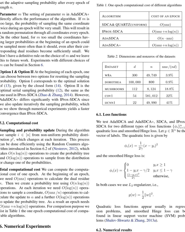
O(nnz +nlog(n))operations. For comparison purpose we list in Table1the one epoch computational cost of compa-rable algorithms.
6. Numerical Experiments
In this section we present results of numerical experiments.
Table 1. One epoch computational cost of different algorithms
ALGORITHM COST OF AN EPOCH
SDCA& QUARTZ(UNIFORM) O(nnz)
IPROX-SDCA O(nnz +nlog(n))
ADASDCA O(n·nnz)
ADASDCA+ O(nnz +nlog(n))
Table 2. Dimensions and nonzeros of the datasets
DATASET d n nnz/(nd) W8A 300 49,749 3.9% DOROTHEA 100,000 800 0.9% MUSHROOMS 112 8,124 18.8% COV1 54 581,012 22% IJCNN1 22 49,990 41% 6.1. Loss functions
We test AdaSDCA and AdaSDCA+, SDCA, and IProx-SDCA for two different types of loss functions{φi}ni=1:
quadratic loss and smoothed Hinge loss. Lety∈Rnbe the vector of labels. The quadratic loss is given by
φi(x) =
1
2γ(x−yi)
2
and the smoothed Hinge loss is:
φi(x) = 0 yix≥1 1−yix−γ/2 yix≤1−γ (1−yix)2 2γ otherwise,
In both cases we useL2-regularizer, i.e.,
g(w) = 1 2kwk
2.
Quadratic loss functions appear usually in regres-sion problems, and smoothed Hinge loss can be found in linear support vector machine (SVM) prob-lems (Shalev-Shwartz & Zhang,2013a).
6.2. Numerical results
We used 5 different datasets: w8a, dorothea, mushrooms, cov1 and ijcnn1 (see Table2).
AdaSDCA The results of the theory developed in Section4
can be observed through Figure1to Figure4. AdaSDCA needs the least amount of iterations to converge, confirming the theoretical result.
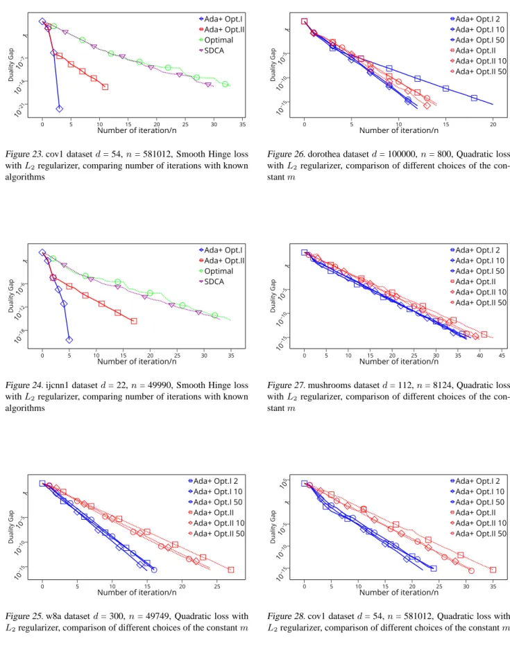
AdaSDCA+ V.S. others We can observe through Figure15
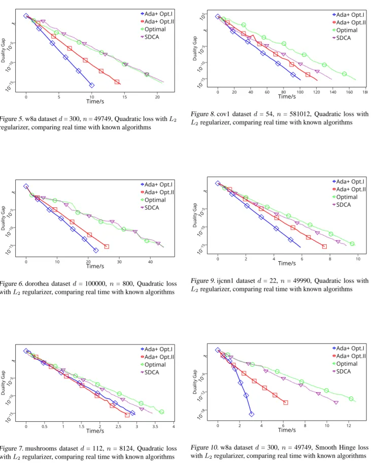
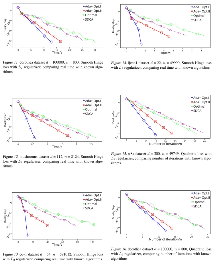
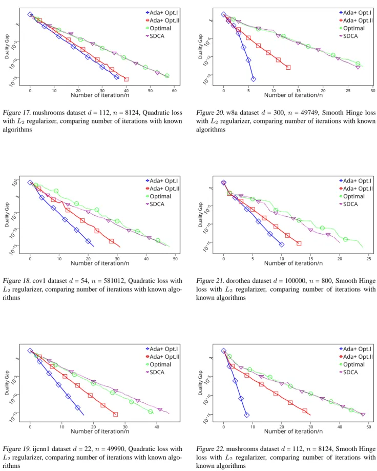
to24, that both options of AdaSDCA+ outperforms SDCA and IProx-SDCA, in terms of number of iterations, for quadratic loss functions and for smoothed Hinge loss func-tions. One can observe similar results in terms of time through Figure5to Figure14.
Option I V.S. Option II Despite the fact that Option I is
not theoretically supported for smoothed hinge loss, it still converges faster than Option II on every dataset and for ev-ery loss function. The biggest difference can be observed on Figure13, where Option I converges to the machine pre-cision in just 15 seconds.
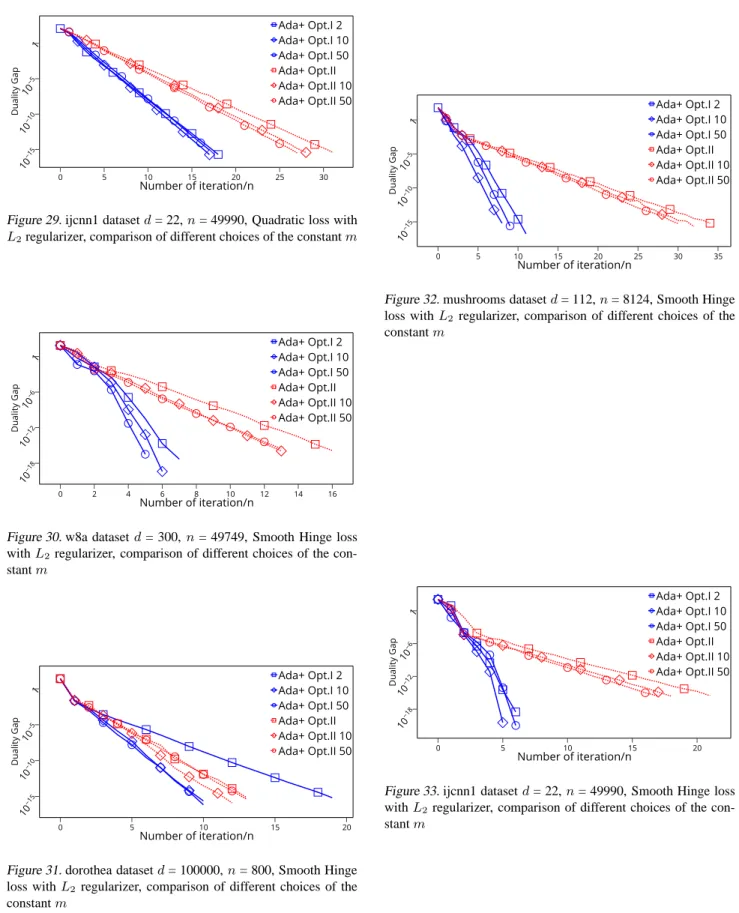
Different choices of m To show the impact of different choices of mon the performance of AdaSDCA+, in Fig-ures25to33we compare the results of the two options of AdaSDCA+ using differentmequal to2,10and50. It is hard to draw a clear conclusion here because clearly the op-timalmshall depend on the dataset and the problem type.
Figure 1. w8a dataset d= 300,n = 49749, Quadratic loss with
L2regularizer, comparing number of iterations with known
algo-rithms
Figure 2. dorothea datasetd= 100000,n= 800, Quadratic loss withL2regularizer, comparing number of iterations with known
algorithms
Figure 3. mushrooms datasetd= 112,n= 8124, Quadratic loss withL2regularizer, comparing number of iterations with known
algorithms
Figure 4. ijcnn1 datasetd= 22,n= 49990, Quadratic loss with
L2regularizer, comparing number of iterations with known
Figure 5. w8a datasetd= 300,n= 49749, Quadratic loss withL2
regularizer, comparing real time with known algorithms
Figure 6. dorothea datasetd= 100000,n= 800, Quadratic loss withL2regularizer, comparing real time with known algorithms
Figure 7. mushrooms datasetd= 112,n= 8124, Quadratic loss withL2regularizer, comparing real time with known algorithms
Figure 8. cov1 datasetd= 54,n= 581012, Quadratic loss with
L2regularizer, comparing real time with known algorithms
Figure 9. ijcnn1 datasetd= 22,n= 49990, Quadratic loss with
L2regularizer, comparing real time with known algorithms
Figure 10. w8a datasetd= 300, n= 49749, Smooth Hinge loss withL2regularizer, comparing real time with known algorithms
Figure 11. dorothea datasetd= 100000,n= 800, Smooth Hinge loss withL2 regularizer, comparing real time with known
algo-rithms
Figure 12. mushrooms datasetd= 112,n= 8124, Smooth Hinge loss withL2 regularizer, comparing real time with known
algo-rithms
Figure 13. cov1 datasetd= 54,n= 581012, Smooth Hinge loss withL2regularizer, comparing real time with known algorithms
Figure 14. ijcnn1 datasetd= 22,n= 49990, Smooth Hinge loss withL2regularizer, comparing real time with known algorithms
Figure 15. w8a datasetd= 300,n= 49749, Quadratic loss with
L2regularizer, comparing number of iterations with known
algo-rithms
Figure 16. dorothea datasetd= 100000,n= 800, Quadratic loss withL2regularizer, comparing number of iterations with known
Figure 17. mushrooms datasetd= 112,n= 8124, Quadratic loss withL2regularizer, comparing number of iterations with known
algorithms
Figure 18. cov1 datasetd= 54,n= 581012, Quadratic loss with
L2regularizer, comparing number of iterations with known
algo-rithms
Figure 19. ijcnn1 datasetd= 22,n= 49990, Quadratic loss with
L2regularizer, comparing number of iterations with known
algo-rithms
Figure 20. w8a datasetd= 300, n= 49749, Smooth Hinge loss withL2regularizer, comparing number of iterations with known
algorithms
Figure 21. dorothea datasetd= 100000,n= 800, Smooth Hinge loss withL2 regularizer, comparing number of iterations with
known algorithms
Figure 22. mushrooms datasetd= 112,n= 8124, Smooth Hinge loss withL2 regularizer, comparing number of iterations with
Figure 23. cov1 datasetd= 54,n= 581012, Smooth Hinge loss withL2regularizer, comparing number of iterations with known
algorithms
Figure 24. ijcnn1 datasetd= 22,n= 49990, Smooth Hinge loss withL2regularizer, comparing number of iterations with known
algorithms
Figure 25. w8a datasetd= 300,n= 49749, Quadratic loss with
L2regularizer, comparison of different choices of the constantm
Figure 26. dorothea datasetd= 100000,n= 800, Quadratic loss withL2regularizer, comparison of different choices of the
con-stantm
Figure 27. mushrooms datasetd= 112,n= 8124, Quadratic loss withL2regularizer, comparison of different choices of the
con-stantm
Figure 28. cov1 datasetd= 54,n= 581012, Quadratic loss with
Figure 29. ijcnn1 datasetd= 22,n= 49990, Quadratic loss with
L2regularizer, comparison of different choices of the constantm
Figure 30. w8a datasetd= 300, n= 49749, Smooth Hinge loss withL2regularizer, comparison of different choices of the
con-stantm
Figure 31. dorothea datasetd= 100000,n= 800, Smooth Hinge loss withL2regularizer, comparison of different choices of the
constantm
Figure 32. mushrooms datasetd= 112,n= 8124, Smooth Hinge loss withL2regularizer, comparison of different choices of the
constantm
Figure 33. ijcnn1 datasetd= 22,n= 49990, Smooth Hinge loss withL2regularizer, comparison of different choices of the
References
Agarwal, Alekh and Bottou, Leon. A lower bound for the optimization of finite sums. arXiv:1410.0723, 2014. Banks-Watson, Alexander. New classes of coordinate
de-scent methods. Master’s thesis, University of Edinburgh, 2012.
Defazio, Aaron, Bach, Francis, and Lacoste-Julien, Si-mon. Saga: A fast incremental gradient method with support for non-strongly convex composite objectives.
arXiv:1407.0202, 2014.
Duchi, John, Hazan, Elad, and Singer, Yoram. Adaptive subgradient methods for online learning and stochastic optimization. Journal of Machine Learning Research, 12(1):2121–2159, 2011.
Fercoq, Olivier and Richt´arik, Peter. Accelerated, parallel and proximal coordinate descent. SIAM Journal on
Opti-mization (after minor revision), arXiv:1312.5799, 2013.
Fercoq, Olivier and Richt´arik, Peter. Smooth minimization of nonsmooth functions by parallel coordinate descent.
arXiv:1309.5885, 2013.
Fercoq, Olivier, Qu, Zheng, Richt´arik, Peter, and Tak´aˇc, Martin. Fast distributed coordinate descent for mini-mizing non-strongly convex losses. IEEE International
Workshop on Machine Learning for Signal Processing,
2014.
Fountoulakis, Kimon and Tappenden, Rachael. Robust block coordinate descent. arXiv:1407.7573, 2014. Glasmachers, Tobias and Dogan, Urun. Accelerated
co-ordinate descent with adaptive coco-ordinate frequencies. In Asian Conference on Machine Learning, pp. 72–86, 2013.
Jaggi, Martin, Smith, Virginia, Takac, Martin, Terhorst, Jonathan, Krishnan, Sanjay, Hofmann, Thomas, and Jor-dan, Michael I. Communication-efficient distributed dual coordinate ascent. In Ghahramani, Z., Welling, M., Cortes, C., Lawrence, N.D., and Weinberger, K.Q. (eds.), Advances in Neural Information Processing
Sys-tems 27, pp. 3068–3076. Curran Associates, Inc., 2014.
Johnson, Rie and Zhang, Tong. Accelerating stochastic gradient descent using predictive variance reduction. In
NIPS, 2013.
Koneˇcn ´y, Jakub and Richt´arik, Peter. S2GD: Semi-stochastic gradient descent methods. arXiv:1312.1666, 2014.
Koneˇcn ´y, Jakub, Lu, Jie, Richt´arik, Peter, and Tak´aˇc, Mar-tin. mS2GD: Mini-batch semi-stochastic gradient de-scent in the proximal setting. arXiv:1410.4744, 2014a.
Koneˇcn ´y, Jakub, Qu, Zheng, and Richt´arik, Peter. Semi-stochastic coordinate descent. arXiv:1412.6293, 2014b. Lin, Qihang, Lu, Zhaosong, and Xiao, Lin. An accelerated proximal coordinate gradient method and its application to regularized empirical risk minimization. Technical Report MSR-TR-2014-94, July 2014.
Liu, Ji and Wright, Stephen J. Asynchronous stochastic coordinate descent: Parallelism and convergence prop-erties. arXiv:1403.3862, 2014.
Loshchilov, I., Schoenauer, M., and Sebag, M. Adap-tive Coordinate Descent. In et al., N. Krasnogor (ed.), Genetic and Evolutionary Computation
Confer-ence (GECCO), pp. 885–892. ACM Press, July 2011.
Lukasewitz, Isabella. Block-coordinate frank-wolfe opti-mization. A study on randomized sampling methods, 2013.
Mahajan, Dhruv, Keerthi, S. Sathiya, and Sundararajan, S. A distributed block coordinate descent method for train-ing l1 regularized linear classifiers. arXiv:1405.4544, 2014.
Mairal, Julien. Incremental majorization-minimization op-timization with application to large-scale machine learn-ing. Technical report, 2014.
Mareˇcek, Jakub, Richt´arik, Peter, and Tak´aˇc, Martin. Dis-tributed block coordinate descent for minimizing par-tially separable functions. arXiv:1406.0328, 2014. Necoara, Ion and Patrascu, Andrei. A random coordinate
descent algorithm for optimization problems with com-posite objective function and linear coupled constraints.
Computational Optimization and Applications, 57:307–
337, 2014.
Necoara, Ion, Nesterov, Yurii, and Glineur, Francois. Ef-ficiency of randomized coordinate descent methods on optimization problems with linearly coupled constraints. Technical report, Politehnica University of Bucharest, 2012.
Nemirovski, Arkadi, Juditsky, Anatoli, Lan, Guanghui, and Shapiro, Alexander. Robust stochastic approximation approach to stochastic programming. SIAM Journal on
Optimization, 19(4):1574–1609, 2009.
Nesterov, Yurii. Efficiency of coordinate descent methods on huge-scale optimization problems. SIAM Journal on
Optimization, 22(2):341–362, 2012.
Qu, Zheng and Richt´arik, Peter. Coordinate descent meth-ods with arbitrary sampling I: Algorithms and complex-ity. arXiv:1412.8060, 2014.
Qu, Zheng and Richt´arik, Peter. Coordinate Descent with Arbitrary Sampling II: Expected Separable Overapprox-imation. ArXiv e-prints, 2014.
Qu, Zheng, Richt´arik, Peter, and Zhang, Tong. Random-ized Dual Coordinate Ascent with Arbitrary Sampling.
arXiv:1411.5873, 2014.
Richt´arik, Peter and Tak´aˇc, Martin. Distributed co-ordinate descent method for learning with big data.
arXiv:1310.2059, 2013a.
Richt´arik, Peter and Tak´aˇc, Martin. On optimal prob-abilities in stochastic coordinate descent methods.
arXiv:1310.3438, 2013b.
Richt´arik, Peter and Tak´aˇc, Martin. Parallel coordi-nate descent methods for big data optimization prob-lems. Mathematical Programming (after minor revi-sion), arXiv:1212.0873, 2012.
Richt´arik, Peter and Tak´aˇc, Martin. Iteration complexity of randomized block-coordinate descent methods for min-imizing a composite function. Mathematical
Program-ming, 144(2):1–38, 2014.
Schaul, Tom, Zhang, Sixin, and LeCun, Yann. No more pesky learning rates. Journal of Machine Learning
Re-search, 3(28):343–351, 2013.
Schmidt, Mark, Le Roux, Nicolas, and Bach, Francis. Min-imizing finite sums with the stochastic average gradient.
arXiv:1309.2388, 2013.
Shalev-Shwartz, Shai and Tewari, Ambuj. Stochastic meth-ods forℓ1-regularized loss minimization. Journal of
Ma-chine Learning Research, 12:1865–1892, 2011.
Shalev-Shwartz, Shai and Zhang, Tong. Proximal stochas-tic dual coordinate ascent. arXiv:1211.2717, 2012. Shalev-Shwartz, Shai and Zhang, Tong. Accelerated
mini-batch stochastic dual coordinate ascent. In Advances
in Neural Information Processing Systems 26, pp. 378–
385. 2013a.
Shalev-Shwartz, Shai and Zhang, Tong. Stochastic dual coordinate ascent methods for regularized loss. Journal
of Machine Learning Research, 14(1):567–599, 2013b.
Tak´aˇc, Martin, Bijral, Avleen Singh, Richt´arik, Peter, and Srebro, Nathan. Mini-batch primal and dual methods for svms. CoRR, abs/1303.2314, 2013.
Tappenden, Rachael, Richt´arik, Peter, and Gondzio, Jacek. Inexact block coordinate descent method: complexity and preconditioning. arXiv:1304.5530, 2013.
Tappenden, Rachael, Richt´arik, Peter, and B¨uke, Burak. Separable approximations and decomposition methods for the augmented lagrangian. Optimization Methods
and Software, 2014.
Trofimov, Ilya and Genkin, Alexander. Distributed co-ordinate descent for l1-regularized logistic regression.
arXiv:1411.6520, 2014.
Wright, Stephen J. Coordinate descent al-gorithms. Technical report, 2014. URL
http://www.optimization-online.org/DB_FILE/2014/12/4
Xiao, Lin and Zhang, Tong. A proximal stochastic gradient method with progressive variance reduction.
arXiv:1403.4699, 2014.
Zhang, Yuchen and Xiao, Lin. Stochastic primal-dual coor-dinate method for regularized empirical risk minimiza-tion. Technical Report MSR-TR-2014-123, September 2014.
Zhao, Peilin and Zhang, Tong. Stochastic optimization with importance sampling. arXiv:1401.2753, 2014. Zhao, Tuo, Liu, Han, and Zhang, Tong. A general theory
of pathwise coordinate optimization. arXiv:1412.7477, 2014a.
Zhao, Tuo, Yu, Mo, Wang, Yiming, Arora, Raman, and Liu, Han. Accelerated mini-batch randomized block co-ordinate descent method. In Ghahramani, Z., Welling, M., Cortes, C., Lawrence, N.D., and Weinberger, K.Q. (eds.), Advances in Neural Information Processing
Appendix
Proofs
We shall need the following inequality.
Lemma 13. Functionf :Rn→Rdefined in (3) satisfies
the following inequality:
f(α+h)≤f(α) +h∇f(α), hi+ 1 2λn2h
⊤A⊤Ah, (18)
holds for∀α, h∈Rn.
Proof. Sincegis 1-strongly convex,g∗is 1-smooth. Pick
α, h∈Rn. Since,f(α) =λg∗( 1 λnAα), we have f(α+h) =λg∗( 1 λnAα+ 1 λnAh) ≤λ g∗( 1 λnAα) +h∇g ∗( 1 λnAα), 1 λnAhi+ 1 2k 1 λnAhk 2 =f(α) +h∇f(α), hi+ 1 2λn2h ⊤A⊤Ah.
Proof of Lemma3. It can be easily checked that the
follow-ing relations hold
∇if(αt) = 1 nA ⊤ i w t, ∀t≥0, i∈[n], (19) g(wt) +g∗(¯αt) = hwt,α¯t i, ∀t≥0, (20) where {wt, αt,α¯t}
t≥0 is the output sequence of
Algo-rithm1. Lett ≥0andθ ∈[0,minipti]. For eachi∈[n],
sinceφi is1/γ-smooth,φ∗i isγ-strongly convex and thus
for arbitrarysi∈[0,1], φ∗ i(−αti+siκti) =φ∗i (1−si)(−αit) +si∇φi(A⊤i w t ) ≤(1−si)φ∗i(−α t i) +siφ∗i(∇φi(A⊤i w t)) −γsi(1−si)|κ t i|2 2 . (21) We have: f(αt+1)−f(αt) (18) ≤ h∇f(αt), αt+1 −αt i + 1 2λn2hα t+1−αt, A⊤A(αt+1−αt) i =∇if(αt)∆αtit + vi 2λn2|∆α t it| 2 (19) = 1 nA ⊤ itw t∆αt it+ vi 2λn2|∆α t it| 2 (22) Thus, D(αt+1) −D(αt) (22) ≥ −n1A⊤itw t∆αt it− vit 2λn2|∆α t it| 2+ 1 n n X i=1 φ∗i(−αti) −n1 n X i=1 φ∗i(−α t+1 i ) =−1 nA ⊤ itw t∆αt it− vit 2λn2|∆α t it| 2+1 nφ ∗ it(−α t it) − 1 nφ ∗ it(− α t it+ ∆α t it ) = max ∆∈R− 1 nA ⊤ itw t∆ − vit 2λn2|∆| 2+ 1 nφ ∗ it(−α t it) −n1φ∗ it(− α t it + ∆ ),
where the last equality follows from the definition of∆αt it in Algorithm 1. Then by letting ∆ = −siκtit for some arbitrarysi∈[0,1]we get: D(αt+1)−D(αt) ≥ siA ⊤ itw tκt it n − s2 ivit|κ t it| 2 2λn2 + 1 nφ ∗ it(−α t it) −1nφ∗it(−α t it+siκ t it) (21) ≥ si n φ ∗ it(−α t it)−φ ∗ it(∇φit(A ⊤ itw t)) +A⊤ itw tκt it −s 2 ivit|κ t it| 2 2λn2 + γsi(1−si)|κtit| 2 2n .
By taking expectation with respect toitwe get:
EtD(αt+1)−D(αt) ≥ n X i=1 pt isi n φ∗ i(−α t i)−φ∗i(∇φi(A⊤i w t)) +A⊤ i w tκt i − n X i=1 pt is2i|κti|2(vi+λγn) 2λn2 + n X i=1 pt iγsi|κti|2 2n . (23) Set si= 0, i /∈It θ/pt i, i∈It (24) Thensi∈[0,1]for eachi∈[n]and by plugging it into (23)
we get: EtD(αt+1)−D(αt) ≥ θnX i∈It φ∗ i(−α t i)−φ∗i(∇φi(A⊤i w t)) +A⊤ i w tκt i −2λnθ 2 X i∈It θ(v i+nλγ) pt i −nλγ |κti|2
Finally note that: P(wt) −D(αt) = 1 n n X i=1 φi(A⊤i w t) +φ∗ i(−α t i) +λ g(wt) +g∗(¯αt) (20) = 1 n n X i=1 φ∗ i(−α t i) +φi(A⊤i w t) + 1 nhw t, Aαt i = 1 n n X i=1 φ∗i(−αti) +A⊤i wt∇φi(A⊤i wt) −φ∗ i(∇φi(A⊤i w t)) +A⊤ i w tαt i = 1 n n X i=1 φ∗ i(−α t i)−φ∗i(∇φi(A⊤i w t)) +A⊤ i w tκt i = 1 n X i∈It φ∗ i(−α t i)−φ∗i(∇φi(A⊤i w t)) +A⊤ i w tκt i
Proof of Lemma4. Note that (13) is a standard constrained
maximization problem, where everything independent ofp
can be treated as a constant. We define the Lagrangian
L(p, η) =θ(κ, p)−η(
n
X
i=1
pi−1)
and get the following optimality conditions:
|κt i|2(vi+nλγ) p2 i = |κ t j|2(vj+nλγ) p2 j , ∀i, j∈[n] n X i=1 pi= 1 pi≥0, ∀i∈[n],
the solution of which is (14).
Proof of Lemma5. Note that in the proof of Lemma3, the
conditionθ∈[0,mini∈Itp
t
i]is only needed to ensure that
si defined by (24) is in [0,1]so that (21) holds. Ifφi is
quadratic function, then (21) holds for arbitrarysi ∈ R.
Therefore in this case we only needθto be positive and the same reasoning holds.