Improving HIV-1 Integrase Inhibitors Prediction Using Hybrid Differential Evolution-Binary Particle Swarm Algorithm

(1)

(2)

Improving HIV-1 Integrase Inhibitors Prediction Using Hybrid Differential

Evolution-Binary Particle Swarm Algorithm

THESIS SUBMITTED IN PARTIAL FULLFILLMENT

OF THE REQUIREMENTS FOR THE DEGREE

MASTER OF SCIENCES

IN

COMPUTER SCIENCE

Author: Matinehalsadat Kashani Moghaddam

CALIFORNIA STATE UNIVERSITY SAN MARCOS

Department of Computer Science

(3)

Abstract

Due to the mutation of HIV enzymes and their resistance against current drugs, drug companies are exploring ways to develop stronger mutant resistant drugs. Dimeric aryl diketo acids have proven to be effective inhibitors to the HIV strand transfer mechanism of HIV-integrase. In order to create the best drug to fight HIV-integrase, it is important to know which features of the diketo acids have the biggest impact on reducing HIV enzyme activity. The use of evolutionary algorithms and predictive models, such as the differential evolutionary – binary particle swarm optimization (DE-BPSO) algorithm and Random Forest used in this research, can help find a small subset of the diketo acid’s chemical descriptors that are best able to predict the reduction in HIV enzyme activity. In this research the development of the DE-BPSO/MLR model is discussed and compared with the results against linear models tested in previous work. Also, through implementing Random Forest and TreeNet the results of linear models are compared with Non Linear models. Comparing both models will help determine which QSAR model yields the most effective HIV-IN inhibitors. Due to the nature of Acquired Immunodeficiency Syndrome (AIDS) and the current treatments’ numerous side effects and rapid emergence of drug resistant variants, maximizing the effectiveness of integrase inhibitors is an important milestone to current HIV research.

(4)

Acknowledgements

First, I would like to express my sincere gratitude to my MSc supervisor, Dr. Ahmad Reza Hadaegh for his continuous support, patience, motivation, enthusiasm, and immense knowledge.

Besides my supervisor, I would like to thank my thesis committee, Dr. Xiang Zhang. His insightful comments and helpful suggestions brought a new spirit to this thesis.

Furthermore, I would like to thank the Department of Computer Science at the California State University, San Marcos.

I wish to thank my classmates and friends. In particular, I would like to thank Richard Galvan and Simi Yusuf for their friendship and support.

Lastly, I would like to thank my close family. My utmost gratitude goes to my parents, Mitra Emamzadeh -Ghasemi and Mojtaba Kashani Moghaddam who have always been my greatest inspiration in life. They have showed me the true meaning of unconditional love. I will always be grateful to them for their strong faith in me and their tremendous support at every stage of my life.

I am thankful for the presence of my beautiful sister, Atieh , in my life. I would have not been the person I am without her pure love and friendship.

Finally, I am very grateful for having my loving and patient husband, Farsheed Mahmoudi, in my life. I appreciate his understanding, guidance and faithful support during all the stages of this MSc very much.

(5)

List of Figures

Figure 1 The workflow of a QSAR model ... 13

Figure 2: QSAR Models... 15

Figure 3.Drug Design ... 18

Figure 4: Outline of the Basic Genetic Algorithm ... 18

Figure 5: Outline of the Basic BPSO Algorithm ... 21

Figure 6: The DE Algorithm ... 22

Figure 7: QSAR model development using (DE-BPSO) ... 26

Figure 8: Representative structures of Aryl -diketo acid ... 27

Figure 9: Distribution of descriptors calculated for feature selection for QSAR development ... 27

Figure 10: General process for RF and TreeNet ... 30

Figure 11: Results by using DE-BPSO Algorithm and Multiple Linear Regression (DE-BPSO-MLR) for developing QSAR model (91 Aryl B-Diketo Acids) ... 33

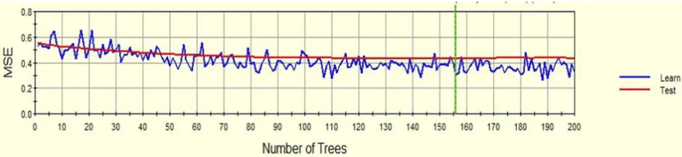
Figure 12: MSE vs. Number of Trees for learning and testing curves in TreeNet ... 36

Figure 13: MSE vs. Number of Trees for the learning curve in Random Forest ... 36

Figure 14: Architecture ... 37

Figure 15: The QSAR Modeling Database ... 38

Figure 16: Main Administrative Dashboard ... 39

Figure 17: Add any defined Entity type to the QSAR database ... 40

Figure 18: Adding a new (Model) entity to the QSAR Database ... 40

Figure 19: The newly added model then becomes available as a configuration option in the client view 40 Figure 20: Models can be changed, i.e. either updated or deleted ... 41

Figure 21: Additional administrator users can be added or changed from the main dashboard ... 41

Figure 22: Creating a New Session ... 41

Figure 23: Select Model Configuration ... 42

Figure 24: Create Session ID ... 43

Figure 25: Create Session ID ... 43

Figure 26: Uploading External Data ... 44

Figure 27: Starting Training Session ... 44

Figure 28: Get Training Status ... 45

Figure 29: Stopping Training Status ... 45

Figure 30: Downloading Training Status ... 46

Figure 31: Restoring an Existing Session ... 46

(7)

List of Tables

Table 1 Averaged Fitness Values of DE-BPSO Parameters... 28

Table 2: Model Performance (DE-BPSO-MLR)-(91 B-diketo acids) ... 32

Table 3: Selected Descriptors in β-Diketo Acid QSAR Model- 91 B-diketo acids (DE-BPSO-MLR) ... 33

Table 4: Descriptors used in QSAR Model (Data set of 37 β-Diketo Acids) ... 34

Table 5: pIC50 variable importance descriptors used in pIC50 using the TreeNet system, ranked by variable importance score ... 35

(8)

1. Introduction

Topic Overview

The human immunodeficiency virus type 1 (HIV-l) is a retrovirus responsible for the acquired immunodeficiency syndrome (AIDS) disease. According to estimates by World Health Organization (WHO), 35.3 million people were living with HIV at the end of 2012. That same year, some 2.3 million people became newly infected, and 1.6 million died of AIDS-related causes (HIV/AIDS, 2013). One of the biggest problems with current HIV drugs on the market is their lack of resistance to the mutation of HIV proteins. Involved in the replication process are three virally encoded enzymes, HIV-Protease, Integrase, and Reverse Transcriptase. The majority of the drugs on the market target the HIV-Protease and Reverse Transcriptase enzymes. In order to develop a stronger HIV mutant resistant drug, it is important to know which physiochemical properties (features) of the drug will lead to the biggest reduction in HIV enzyme activity.

Role of Data mining and Machine Learning in Drug Design

Data mining is a multi-disciplinary field which is a combination of machine learning, artificial intelligence statistics and database technology. By means of data analysis, Data mining attempts to explain the past and predict the future.

Machine learning is the study of computer algorithms to learn in order to improve automatically through experience. Machine learning and data mining have some similarities. Both systems look for patterns by searching. However, in data mining applications data is extracted for human comprehension, in machine learning that data is used to improve the program's own understanding. Machine learning programs detect patterns in data and adjust program actions accordingly.

The objective in Data mining is to reduce complexity and extract, or mine, as much relevant and useful information from a large data set as possible. Data mining uses machine learning as well as statistical and visualization methodologies. The result is discovery and representation knowledge in a form that is easily understood by humans.

In order to deal with the huge amounts of biological information of different forms that the biopharmaceutical industry collects, industry is increasingly employing a variety of data-mining methodologies. Data mining tools are backbone of Computer aided drug designing. It is used for feature

(9)

selection, model building and reducing the feature dimension by removing similar and non-significant descriptors.

Model Development

Quantitative structure-activity relationship (QSAR) models and evolutionary algorithms can be used in combination to determine which chemical descriptors of a drug will lead to the biggest reduction in enzyme activity. Given a set of quantitative features and an associated target variable, QSAR models determine the relationship each feature has with the target variable (Csermely, 2013) (Ko, 2012).

For example, if feature X is decreased, a QSAR model will determine whether the target variable should increase or decrease. In our case, the set of features is the chemical descriptors that make up a drug and the target variable is the scaled concentration level of the drug at which point the enzyme activity is reduced by 50%. Evolutionary algorithms help in selecting a subset of features that will have the biggest impact on the predictability of a QSAR model. Through the use of QSAR models and evolutionary algorithms, we can create a model with the decent set of features to predict the effect a drug has on enzyme activity and thus how well the drug should be able to overcome the mutation of HIV proteins. Knowing which chemical descriptors have the biggest impact on enzyme activity helps drug manufacturers focus on the descriptors that will produce the best HIV mutant resistant drug.

Overview of a Model

A model can be thought of as an equation that predicts the outcome of something. A simple example of a model is a weighted average. The feature values, or x’s, in the equation represent different features (independent variables) and the weights, w’s, represent how each feature relates to a target variable (dependent variable). In order to train a model to predict a target variable as accurately as possible, samples must be provided, each with a set of features and an associated target value. Training of a model is done in an iterative manner. To initialize a model, a random weight, a, b, c, … are assigned to features X1, X2, X3, …..

Y = aX1, bX2, cX3, …+ error

Using these weights, the value of the target variable for each sample is predicted. The error of each prediction is then calculated. Using the overall error, weights are updated in such a way that the next time predictions are calculated, the overall error should decrease.

(10)

Research Contribution

In this Thesis, the related work of the linear and non-linear approaches has been studied. The focus is on inhibitors that can stop the activity of HIV-Integrase by using both linear (MLR) and non-linear models (RF and TreeNet) along with evolutionary algorithms(DE-BPSO) to select the best features that lead to the most accurate prediction of drug performance. Also, the result is compared with the results of the linear approach that had been previously done on the data. The architectural model of the work is shown in Error! Reference source not found..

The work has been currently executed with 91 drugs extracted from -Diketo compound. The metric we will use for drug performance is the drug’s pCI-50 level, or the scaled concentration of the drug at which point the HIV enzyme activity is reduced by 50%. Using models to select the best features will help speed up the drug development process and reduce costs. Without using models, drug research firms would need to test many different combinations of drug features. This is practically not possible because testing all combination is an NP-complete problem which is not accepted at this stage.

The second part of this thesis is to develop a repository database where data can be submitted and appropriate programs can be chosen to execute on a set of data to generate models. I developed the back-end database, set up the constraints , and designed efficient front-end tool where clients can submit their data and receive the results within acceptable time frame.

In brief this research makes the following contribution:

 It improves the evolutionary algorithm (DE-BPSO) to produce better results compare to the work that has been previously done (Qi Shen, 2004) (Micheal Fernandez, 2010).

 It uses data mining tools such as commercial product of Salford Predictive Modeling (SPM) to do non-linear modeling using “Random Forest” and “Tree Net” (Salford Systems).

 It compares and discusses the results generated from the linear models and non-linear models on the data

 It creates a repository database (with capability of becoming a warehouse) that can perform linear and non-linear modeling using variety of algorithms. The database can be extended to

(11)

link to existing free products such as “R” and “Rattle” and commercial products such as “Salford Productive Modeling” tools to do the modeling.

The rest of this paper is organized as follow. Chapter 2 provides the related work on QSAR, and machine learning related to this thesis. It discusses all the information to linear and non-linear models in detail. Chapter 3 explains about the modeling tools and evolutionary algorithms. It discusses how commercial tools such as “Salford Predictive Modeling” works. Chapter 4 illustrates the architectural model of our work. It explains the steps required to do linear modeling with evolutional algorithms, and the general picture of non-linear models we plan to address in this paper. The results of the implementations of the models are discussed and compared in chapter 5. Chapter 6 presents the design and implementation of repository database. Finally, Chapter 7 provides the conclusion and points out the related open problems.

(12)

2. Background:

2.1 QSAR in Bioinformatics

The biological activity of a chemical compound is a function of its physiochemical properties. It was demonstrated in the early 1960, by the pioneer work of Hansch et al[Parlodos,2007]. Examples of these physiochemical properties include the dipole moment, molecular weight, total energy, solvent accessible area, and so on. The physiochemical properties are called quantitative structure-activity relationship (QSAR) and are usually derived from the compound’s structure. A number of different QSAR properties have been developed so far and they are used widely to model and analyze chemical compounds within the pharmaceutical industry (Wang, 2005).

Depending on the property, the amount of time required to compute QSAR properties varies. Some of them such as molecular weight can be computed very fast, while some others such as dipole moment and total energy can be performed only for small datasets and require time-consuming numerical simulations.

2.2 QSAR and Computational Chemistry

In computational chemistry, molecular structures are represented as numerical models and their behavior is simulated with the equations of quantum and classical physics. Scientists use specific programs to generate and present molecular data such as energies, geometries and associated properties (electronic, spectroscopic and bulk). A table is the standard model for presenting and employing these data. In this table, rows are to present compounds and related columns are for presenting molecular properties (descriptors).

A QSAR is used early in the drug development stage to filter out potential failures. For a series of compounds, the role of QSAR is to find the consistent relationships between the values of molecular properties and the biological activity. These rules are then used to evaluate new chemical entities. In a simple word QSAR is a mathematical relationship between biological activity of molecular system and its geometric and chemical characteristics:

Activity = f (molecular or fragmental properties)

QSAR works on the assumption that structurally similar compounds have similar activities. It attempts to understand drug action, design new compounds, and screen chemical libraries. Therefore, QSAR has both predictive and diagnostic abilities. A QSAR generally takes the form of a linear equation:

(13)

Biological Activity = Const + (C1 * P1) + (C2 * P2) + (C3 * P3) +…

For each molecule in the series, the parameters P₁ through P_n are calculated. The coefficients C1 through Cn are computed by fitting variations in the parameters and the biological activity.

2.3 General workflow of developing a QSAR model

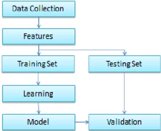
Figure 1: The workflow of a QSAR model

A QSAR workflow starts with collecting data for the property of interest while considering the quality of the data which means excluding the low-quality data. Representation of the collected molecules is done by using features such as molecular descriptors which describes important information of the molecules. Then, the full data set is divided into a training set and a testing set for correction and validation of the QSAR model. The optimal model is the result of searching for the optimal modeling parameters and feature subset simultaneously. Finally, the finalized model built from the optimal parameters would go through validation with a testing set to ensure that the model is correct and useful, (Faulon, 2010).

2.4 Methods for constructing QSAR

QSAR models are constructed by various modeling methods. No method is useful for all QSAR problems and the simplest method that provides the desired performance level should be used.

(14)

 Methods for regression problems which include: Multiple Linear Regression (MLR), Partial Least Squares (PLSs), Feed forward Back propagation Neural Network (ANN), General Regression Neural Network, Gaussian Processes (GP).

 Methods for classification problems such as Support Vector Machine (SVM), Logistic Regression (LR), Linear Discriminant Analysis (LDA), Decision Tree and Random Forest (DT), k-Nearest Neighbor (KNN), Probabilistic Neural Network (PNN).

Three components are required for the development of a QSARs model:

1) A data set that provides activity (usually measured experimentally) for a group of chemicals (i.e., the dependent variable). This group of chemicals is typically defined by some selection criteria.

2) A structural criteria (structure-related property data) set for the same group of chemicals (i.e., the independent variables).

3) A method of relating these two data arrays (usually a statistical analysis method). Methods for relating structure to activity range from the simple linear regression, through more complex approaches such as partial least squares analysis to the most complex machine learning techniques such as neural networks.

2.5 Linear vs Non-Linear Models

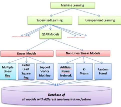
In general, machine learning techniques are divided into two general areas of supervised and unsupervised learning. QSAR models are supervised learning models that are used in the chemical and biological sciences and engineering.

When creating a supervised model, there are two types of models, linear and non-linear. With linear models, each feature is assigned a weight. A target value can be predicted by calculating the weighted average. Linear models are structured in such a way that when you increase the value of a feature by a certain amount, the target variable will change by a proportional amount. The proportional amount is determined by the weight of the feature in the model. For example, if the weight of a feature has a value of 1.5 and the feature value changes by 2.0, the target variable prediction will increase by 3.0. With non-linear models, similar changes in a feature’s value will have a varying effect on target variable depending on the feature’s beginning value. Non-linear models are often better than linear models at predicting a target variable because they can better adjust to the data.

Examples of QSAR linear models are MLR, PLSR, and SVM. Examples of non-linear models are RF, ANN, and KNN.

(15)

Figure 2: QSAR Models

2.5.1 Linear Models

Multiple Linear Regression (MLR)

MLR method is used for studying the relationship between a dependent variable and two or more independent variables. A multiple linear regression model with two predictor (Independent) variables, X1 and X2 is shown as:

Y= β

0

+ β

1

X

1

+ β

2

X

2

+ ϵ

Partial Least Square Regression (PLSR)

PLSR is an extension of the MLR model. As in MLR, the main purpose of PLSR is to build a linear model. PLSR has been used in various disciplines where predictive linear modeling, especially with a large number of predictors, is necessary. MLR can be a good method to use when three conditions are present: the number of factors is few, factors are not considerably redundant (collinear), and factors have a well-understood relationship to the responses. However, in the absence of any of these three

(16)

conditions, MLR can be ineffective or incorrect. When the factors are many and highly collinear, PLSR is a good method to use for constructing predictive models. This is when the importance is on predicting the responses and determining the underlying relationship between the variables is not the main purpose.

Basically, MLR can be used with very many factors. But, when the number of factors gets too large (for example, greater than the number of observations), over-fitting is likely to happen. It happens when we get a model that fits the sampled data perfectly but that will fail to predict new data well. In such situation, although there are many obvious factors, there may be only a few underlying or hidden factors that account for most of the variation in the response. The general idea of PLS is to try to extract these hidden factors, accounting for as much of the obvious factor variation as possible while modeling the responses well.

Support Vector machine (SVM)

The support vector machine (SVM) is a data-driven method which is used for solving classification tasks. Generally, it results in lower prediction error compared to classifiers based on other methods like Artificial Neural Networks (ANN), especially when there is large numbers of features for sample description. SVM always tries to classify objects with large assurance, which prevents from over-fitting while no strong assumption on the data generation process (contrary to Bayesian approaches). User of Support Vector Machines is able to prevent over-fitting by controlling the margins. SVM minimizes the expected generalization error rather than apparent error. Theoretical bounds on the expected

generalization error are given. Therefore, it is an efficient method [ĆWIKLIŃSKA-JURKOWSK, 2009].

2.5.2 Non-Linear Models

Decision Tree

Decision trees are used for constructing classification or regression models in the form of a tree structure. It can handle both categorical and numerical data. Decision tree divides a dataset into smaller and smaller subsets and simultaneously a related decision tree is incrementally built. As the final result a tree with decision nodes and leaf nodes will be generated. A decision node contains two or more branches Leaf node represents a classification or decision. The root node in a tree is the top most decision node which represents the best predictor.

(17)

Random Forest

Random Forests also thought of as a form of nearest neighbor predictor, are an ensemble learning method for classification and regression. Random Forests are an ideal tool for making predictions since they do not over-fit as the result of the law of large numbers. To make them accurate classifiers and regressors the right kind of randomness should be introduced. At training time, Random Forest builds a number of decision trees and outputting the class that is the mode of the classes output by individual trees. The basic principle is that a group of “weak learners” can come together to form a “strong learner”. Random Forests are a combination of tree predictors. Each tree depends on the values of a random vector experimented independently with the same distribution for all trees in the forest.

Artificial Neural Network

An artificial neutral network (ANN) is based on the biological neural network, such as the brain.

An ANN consists of a network of artificial neurons, known as "nodes". There are three types of neurons in an ANN, input nodes, hidden nodes, and output nodes. These nodes are connected to each other. Based on their strength, inhibition (maximum being -1.0) or excitation (maximum being +1.0), the strength of their connections to one another is assigned a value. The high value of the connection indicates that there is a strong connection. A transfer function is built in within each node's design.

K-Nearest Neighbor

KNN is used in statistical estimation and pattern recognition as a non-parametric technique. It is a simple algorithm to store all available cases and classify new cases based on a similarity measure (e.g., distance functions).

2.6 Models and Methods used in this thesis

In this thesis, the non-linear RF and linear model Multiple Linear Regression (MLR) are developed to help find a subset of the diketo acid’s chemical descriptors that are best able to predict the reduction in HIV enzyme activity. The models are implemented by the Evolutionary Algorithms (EA), differential evolutionary - binary particle swarm optimization (DE-BPSO). Random Forest and TreeNet serve as a predictive modeling tool that can address multiple outcomes and numerous variables. Then, the results are compared against other linear and non-linear models tested in previous works [GeneKo,2012] . Comparing models will help determine which QSAR model yields the most effective HIV-IN inhibitors.

(18)

3. Methods

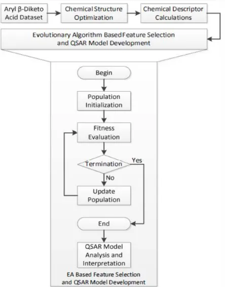
3.1 Evolutionary Algorithms as feature selection techniques for the QSAR modeling

In recent times, a large number of biologically inspired algorithms have been invented, and are being used for solving many complex tasks. They have successfully been used in many bioinformatics problems that need intelligent search, optimization and machine learning approaches (Kelemen, 2008).

Figure 3.Drug Design 3.1.1 Genetic Algorithms

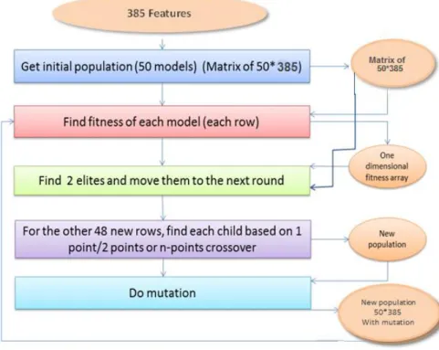
Genetic algorithms are randomized search and optimization techniques conducted by the principles of evolution and natural genetics which are producing near optimal solutions. GA’s are executed iteratively on a set of coded solutions, called population, with three basic operators: selection/reproduction, crossover, and mutation.

(19)

Algorithm initiates with a set of solutions (population). Solutions from one population are taken and used to create a new population. The hope is that the new population will be better than the old one. Solutions which are selected to build new solutions (offspring) are selected according to their fitness. The more appropriate they are the more chances they have to reproduce. This is reiterated until some condition is satisfied (for example number of populations or improvement of the best solution).

1. [Start] Generate random population of n solutions ( rows)

2. [Fitness] Evaluate the fitness f(x) of each row in the population. The closer f(x) is to zero, the better is the MSE. MSE is the mean square error that is the sum of the square of target value minus the predictive value of f(x).

3. [New population] Create a new population by repeating following steps until the new population is complete:

a) [Selection] Select two of the best parent rows from a population according to their fitness (the lower is the fitness, the bigger chance to be selected)and move them to the new population

b) [Crossover] With a crossover probability cross over the parents to build a new offspring (children).

c) [Mutation] With a mutation probability mutate new offspring. Mutation value should be very small number close to zero (ex: 0.02)).

d) [Accepting] Place new offspring in a new population

4. [Replace] Use new generated population for a further run of algorithm

5. [Test] If the end condition is satisfied, stop, and return the best solution in current population 6. [Loop] Go to step 2

3.1.2 Particle Swarm Optimization

Particle swarm optimization (PSO) simulates the behaviors of bird flocking. In PSO, each single solution is like a "bird" that is in the search space looking for food. This single solution is called "particle".

Particles generally move toward the target. The position of each particle is determined based on three data: personal /local best (pbest), global best (gbest) and the velocity of the particle. Each particle has a local best which is the best position a particle has had relative to the target. gbest is the best position obtained so far by any particle in the population and the velocity determines the direction and speed of the particle toward the target.

(20)

A particle also has a measure of the quality of its current position, the particle’s best known position (that is, a previous position with the best known quality), and the quality of the best known position. After finding the two best values, the particle updates its velocity and positions according to the following equation (a) and (b):

v[ ]=v[ ]+c1*rand( )*(pbest[ ]-present[ ])+c2*rand( )*(gbest[ ]-present[ ]) (a)

present [ ] = present[ ] + v[ ] (b)

where v[ ] is the particle velocity, present[ ] is the current particle (solution) and rand ( ) is a random number between (0,1). c1, c2 are learning factors. Usually c1 = c2 = 2. (pbest[ ] and gbest[ ] are defined as stated before).

The velocity is calculated based how far the particle is away from the target. The direction is set toward the target where particle (bird) finds food. The further the article from the target the higher is its speed. PSO algorithms are usually using population topologies, or "neighborhoods". They are smaller, localized subsets of the global best value. These neighborhoods can include two or more particles which are preset to act together, or subsets of the search space that particles happen into during testing. The use of neighborhoods often help the algorithm to avoid getting stuck in local minima [14].

A discrete binary version of PSO for binary problems has been introduced by Kennedy and Eberhart [15]. In their model a particle will decide on "yes" or "no", "true" or "false", "include" or "not to include" etc. Also a real value in binary search space can be represented by this binary. It is not just the interpretation of the velocity and particle paths that changes for the binary PSO. The meaning and behavior of the velocity clamping and the inertia weight is also different from the real-valued PSO. Actually, the effects of these parameters are the opposite of those for the real valued PSO (R.W.Kennard, 1969).

In continuous version of PSO large numbers for maximum velocity of the particle promote exploration. But in binary PSO, even if a good solution is found, small numbers for V max encourages exploration,. And if max V = 0, then the search changes into a pure random search. Exploration is limited by large values for V max.

Updating the particle’s personal best and global best is the same in the binary PSO and in continuous version. The main difference between binary PSO with continuous version is that velocities of the particles are rather defined in terms of probabilities that a bit will change to one. Based on this definition a velocity must be limited within the range [0,1] (Mojtana Ahmadia Khanehsar, 2007). The pseudo code is as follows:

(21)

for each particle:

initialize particle do:

for each particle:

calculate fitness value *

if the fitness value is better than the best fitness value(pbest) in history then set current value as the new pbest

end for

for each particle:

find in the particle neighborhood, the particle with the best fitness calculate particle velocity according to the velocity equation(1) apply the velocity constriction

update particle position according to the position equation (2) apply the position constriction

end for

while (maximum iterations or minimum error criteria is not attained) *Calculating Fitness value:

(22)

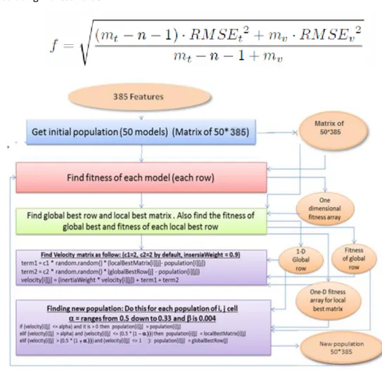
The root mean square error of the training (RMSEt ) and validation (RMSEv ) sets is designed to

decrease the effects of over- fitting. “m “ refers to the number of samples in the training (t) and validation (v) sets, and “n” refers to the number of descriptors in the model .

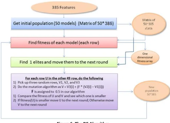
3.1.3 Differential Evolution Algorithm

The DE algorithm is a population based algorithm and like genetic algorithms it uses crossover, mutation and selection. The main difference is that DE relies on mutation operation while genetic algorithms depend on crossover. This main operation is based on the differences of randomly sampled pairs of solutions in the population. As a search mechanism, the algorithm uses mutation operation and to guide the search toward the potential regions in the search space the selection operation is used.

The main steps of the DE algorithm are Initialization, Evaluation, (Repeat: Mutation, Recombination, Evaluation, Selection, until the termination criteria are met. We have used a common simple approach of DE algorithm that is shown below.

(23)

for each particle:

initialize particles randomly do:

- find the fitness of all particles

- find the elite row and move it to the next round - for each particle U:

- select three random distinct rows V1, V2, and V3

- calculate V[ ] = V3[ ] + F (V2[ ] – V1[ ])Calculate fitness value - if (fitness of U is better than V

move U to the next round else

move V to the next round. end for

3.1.4 Differential Evolution – Binary swarm Optimization algorithm (DE-BPSO)

To create the descriptor subsets which are then used in the development of quantitative structure-activity relationship (QSAR) models, a hybrid differential evolution-binary particle swarm optimization (DE-BPSO) algorithm is suggested as a feature selection algorithm:

1) First the BPSO is used as a feature selection algorithm (according to Figure 5: Outline of the Basic BPSO Algorithm). In the first generation, the velocity and position vector of BPSO are initialized according to:

(1-a)



is the probability of selecting a descriptor. To retain the total number of selected descriptors low for each particle we have chosen



= 0 .01.

In previous research, they had 10% of the particles to search the space randomly. The goal is to overcome local optima convergence issues [GeneKo,2012]. Instead of a random particle search, in DE-BPSO the set of rules have been used to incorporate a positional bit mutation factor:

(24)



is the percent chance of flipping the position bits. In this research, to find its optimal value and compared it to the original BPSO algorithm (in with 10% of the particles randomly searching the descriptor space according to the (1-a )rules ),



is varied from 0 to 0.05 in increments of 0.001[GeneKo,2012].

2) Next, the velocities of the particle swarm is developed using DE. The purpose is obtaining the position vector using the above rule. These rules are applied to calculate the velocity vector Vi of each individual particle at each iteration :

𝑣𝑖` = 𝑣𝑎+ 𝐹(𝑣𝑏− 𝑣𝑐) (2-a) 𝑣𝑖𝑑 = { 𝑣𝑖𝑑, 𝑖𝑓 𝑟𝑎𝑛𝑑(0, 1) < 𝐶𝑅 𝑣_𝑖𝑑` , 𝑜𝑡ℎ𝑒𝑟𝑤𝑖𝑠𝑒 (2-b)

Then according to the set of rules in Eq. (2-b) the values of the position vector Vi is computed.

In this research, to get the optimal DE parameters, F and CR were varied from 0.1 to 0.9 in increments of 0.2 using the optimal value of



from the BPSO algorithm in Eq. (1-b) found previously[GeneKo,2012].

DE-BPSO was found to perform better than the standalone BPSO algorithm. The DE-BPSO algorithm was then used to develop multiple linear regression models for the analysis of aryl β-diketo acid compounds for the inhibition of HIV-1 integrase. This algorithm is used as the feature selection method to select the features with the most significant influence on the compounds for the inhibition of HIV-1 integrase. In this research we are working with 91 aryl β-diketo acid compounds which is more than the twice of the compounds have been previously analyzed in other researches.

(25)

3.2 Data mining tool used in this research

Salford Predictive Modeler software suite

The SPM Salford Predictive Modeler® software suite is an analytics and data mining platform. This software is used for creating predictive, descriptive, and analytical models from databases.

The SPM helps to accelerate the process of model building by conducting substantial portions of the model exploration and refinement process for the analyst. Both Salford Systems Predictive Modeler Random Forest and TreeNet systems are automated machine learning technique that are constructed from a defined or randomized number of decision trees, and are commercially developed systems. SPM combines four software products into a single suite. It includes:

 MARS (Multivariate Adaptive Regression Splines):

o MARS is an extension of ANN. It builds its model by piecing together a series of straight lines with each allowed its own slope. This software while capturing essential nonlinearities and interactions, prepares results in a form similar to traditional regression. MARS can trace out any pattern detected in the data.

 CART (Classification and Regression Trees):

o CART is the classification tree that has developed the entire field of advanced analytics and data mining. CART is designed for both non-technical and technical users. It can quickly reveal the important data relationships that could remain hidden using other analytical tools.

 Random Forests:

o Random Forests is a bagging tool. Random Forest helps multiple alternative analyses, randomization strategies, and ensemble learning to produce more accurate models. It spots outliers and anomalies in data, displaying proximity clusters, identifying important predictors, predicting future outcomes, replacing missing values with imputations , discovering data patterns and providing insightful graphics.

 TreeNet:

o TreeNet is an extension of Random Forest and in many cases it works better than Random Forest. Experiments have shown that TreeNet has good performance for both regression and classification. TreeNet’s level of correctness usually cannot be achieved by single models or by ensembles such as bagging or conventional boosting. The algorithm typically generates thousands of small decision trees built in a sequential error–correcting process to converge to an accurate model.

(26)

4. Models

4.1 Differential Evolution-Binary Particle Swarm Optimization Algorithm coupled with

linear Models

DE-BPSO Optimization Algorithm coupled with linear Models (MLR, SVM, PLSR) has been used for the Analysis of Aryl -Diketo Acids for HIV-l Integrase Inhibition.QSAR models are generated according to the flowchart in Figure 7: QSAR model development using (DE-BPSO)

Figure 7: QSAR model development using (DE-BPSO)

pIC₅₀ represents an inhibition and activation measure in log units for dose-dependent assays.

pIC₅₀ = -log(IC₅₀). IC₅₀ represents the compound/substance concentration required for 50% inhibition. So, the larger pIC50 means the more potent compound.

(27)

In this research, to identify the physiochemical properties conducive for inhibition, a series of 91 aryl, -diketo acids with high experimental inhibitory activities are analyzed , in terms of pIC50, towards the strand transfer reaction of HIV-l integrase Figure 8: Representative structures of Aryl -diketo acid

Figure 8: Representative structures of Aryl -diketo acid

This research, we considered 385 constitutional, geometrical, topological, electrostatic, and quantum-chemical descriptors for development of QSAR model. All descriptor values were rescaled to have a zero mean and a standard deviation of one.

The dataset is divided randomly into a training, validation, and test set with 55, 18, and 18 compounds in each set.

Figure 9: Distribution of descriptors calculated for feature selection for QSAR development

Evolutionary algorithm (DE-BPSO) has been used as the feature subset algorithm which serves as input to QSAR Models.

(28)

Previous studies have shown that using the hybridized form of DE and BPSO for building QSAR

models result in better descriptor search performance comparing to using the existing BPSO.

To conclude the ideal parameters for the BPSO and DE-BPSO feature selection algorithms on this dataset, 500 simulations were run for each of the variable parameters and averaged the fitness over 2000 generations [GeneKo,2012].

F=scaling Factor, CR = Crossover Rate

Table 1 Averaged Fitness Values of DE-BPSO Parameters

Because of their simplicity of mechanistic interpretation, linear methods are common modeling methods for QSAR. However, non-linear models such as artificial neural networks, Random Forest or support vector machines may provide a better predictive model.

So, in this research the linear based QSAR models (MLR, SVM, PLSR) coupled with DE-BPSO algorithm are improved and the results have been compared with the result of non-linear models, Random Forest and TreeNet.

4.2 Non-linear models Random Forest and TreeNet

In this research, to determine new compounds with higher inhibitory effects towards HIV-l Integrase, Non-linear models Random Forest and TreeNet are used as predictive tool.

Through implementing Random Forests and TreeNet, 91 β-diketo acids is studied which have been shown experimentally to inhibit the strand transfer reaction of HIV-1 Integrase. The biological activity of each molecule was reported in terms of pIC50, a measure of half the maximal inhibitory concentration. A total of 385 constitutional, geometrical, topological, electrostatic, and quantum-chemical descriptors were considered for the study. (Figure 9: Distribution of descriptors calculated for feature selection for QSAR development

By developing a non-linear QSAR model, Random Forest and TreeNet will yield new relationships that will propose new inhibitors. After running each system with our data, a few statistical values, such as R2 (coefficient of variation) and MSE (mean-squared error), are computed and compared to the

(29)

classification and regression linear QSAR models. These values aid in determining which models provide more specific and effective inhibitory drug proposals.

Random Forest

Random forest algorithms, in general, begin with building the first tree (parent tree), which sorts data through a sequence of determining nodes [Breiman&Cutler]. First, each tree randomly selects 60% of the descriptors and keeps the remaining 40% for out-of-bag testing.

Eventually, each data object being sorted will reach a bottom-leaf node in each tree, which represents the variable importance score, and is comparable to a decision-tree process. Those variable

importance scores are averaged, and non-sorted data (out-of-bag) are used to test the proposed

model’s accuracy. Once the forest has been built, all variables are listed by variable importance score. A random forest builds 500 trees simultaneously, and each tree is built independently of each other. Then, it takes the average of all trees combined to propose a model. If the MSE is relatively small, then there is less deviation among the coordinates in the non-linear model then the linear models. If the R2 value is closer to 1, or greater than the linear models R2 value, then the non-linear model predicts the curve better than the linear model could predict the linear line.

TreeNet

TreeNet, although just an improved version of the random forest algorithm, has a few distinctive features that yield more precise and decisive results. It builds trees, in a similar decision-tree fashion, but it cannot grow the 2nd tree until you have the results of the first tree because the output of the previous tree is required to build additional trees. It required that the T+1st st tree can only be built if the Tth tree results have been found. This is an active rule to prevent two identical trees to be built, thus maximizing predictive findings. Also, TreeNet automatically handles missing data values within data sets, whereas random forests cannot excuse missing data, and falsely calculates statistical values in return. Like random forests, however, if the Mean Square Error (MSE) is relatively small, then there is less deviation among the coordinates in the non-linear model than the linear models. If the R2 value is closer to 1, or greater than the linear models R2 value, then the non-linear model predicts the curve better than the linear model could predict the linear line. R2 is the coefficient of determination which

(30)

represents the goodness of fit of a model. It shows how close the result is to the fitted regression line. An R2of 1 indicates that the regression line perfectly fits the data.

In this research, Salford System Predictive Modeler (SPM) has been used. SPM Random Forest and TreeNet systems are automated; machine learning techniques based on a defined or randomized number of decision trees, and are commercially developed systems. Like classification and regression, Random Forest and TreeNet serve as a predictive modeling tool that can address multiple outcomes and numerous variables. A flow chart is represented below that depicts the general process for both Random Forest and TreeNet (Figure 10: General process for RF and TreeNet (Dan Stienber).

Figure 10: General process for RF and TreeNet

5. Results

In this chapter, we discuss the results of developing the linear QSAR models and non-linear

QSAR models, Random Forest and TreeNet in detail. We reviewed the results of both linear and

non-linear models to provide a comprehensive comparison. The results of linear and non-

linear models are covered in details in the following sub-sections.

5.1 The result of developing linear QSAR models

A total of 385 constitutional, geometrical, topological, electrostatic, quantum-chemical

descriptors were considered for the study. The dataset is divided into a training (n=55),

validation (n=18), and test (n=18) set using the Kennard Stone algorithm (R.W.Kennard, 1969).

This ensures maximization of the chemical space during model training and accurate tests

within the space.

DE-BPSO Algorithm is used to select the individual descriptors. Machine learning models are

then developed from each of the selected descriptor sets by each individual particle. The fitness

(𝑐𝑜𝑠𝑡) of the selected descriptors is measured by the RMSE, sample size (𝑚) of both the training

(31)

(𝑡) and validation (𝑣) set, number of descriptors in the model (𝑛), and a parsimonious penalty

factor

.

Over-fitting vs. Under-fitting

One of major goals of any Machine Learning method is to provide solutions that perform well

not only on the cases used for learning but also on cases never seen before. This is known as

generalization, how well a model performs on new data, and failure to do so is called

over-fitting. Over-fitting occurs when a solution performs well on the training cases but poorly on the

testing cases. When over-fitting starts to occur the search process is stopped. This points out

that the underlying relationships of the whole data were not learned, and instead a set of

relationships existing only on the training cases were learned, but these have no

correspondence over the whole known cases.

In simple words, Over- fitting is when model is too complex and test errors are large although

training errors are small. There should be always a balance between good classification of the

training set, and good classification of future objects (generalization performance). Over-fitting

means fitting too much the training data, which reduces the generalization performance. This is

very important in large dimensions, or with complex non-linear classifiers. On the other hand,

Under-fitting is when model is too simple and both training and test errors are large. Both

over-fitting and under-over-fitting lead to poor predictions on new data sets.

Understanding these two phenomena allows to thread the needle and go into the space

between the two extremes. It is in this gap where the model has predictive power in the

validation set lies.

The role of value of

is to control the balance between finding models with over-fit and

under-fit and must be monitored to find a value under-fit for a given dataset. Through previous researches

by trial and error, for this data set, it has been found out that



= 3.3 to be suitable for the EA to

obtain predictive QSAR models.

To evaluate the MLR models generated from the descriptors selected by the EA, we should use

fitness function. The fitness function is designed to prevent over-fitting and minimize the

number of descriptors in the model.

(32)

The top ranked models with the lowest cost are analyzed and interpreted to understand the

physiochemical properties of dimeric aryl diketo acids conducive for biological activity.

In our simulations we found the optimal values as



= 0.004, F = 0.7, CR = 0.7) and used them

to develop models for the analysis of



-aryl -diketo acids, (

Table 1 Averaged Fitness Values of DE-BPSO Parameters

)The population size in the particle swarm is 50 individuals and we had

1000 generations for the DE-BPSO feature selection algorithm.

Specifically, each model is evaluated in terms of the coefficient of determination, R

2

, mean

squared error (MSE) and root-mean squared error (RMSE). To calculate R

2

for all models, we

use the following definition, whereby

y

represents the target’s mean value:

It should be noted that this version of R

2

would be negative if predictions are poorer than

always forecasting the mean. Basically, R

2

represents the amount of variation of the

dependent variable explained by the model so, it is considered as singular measure of

predictive accuracy.

MLR models with high correlation (R

2

> 0.6), high predictive correlation with the validation (R

2 v

> 0.5) and test (R

2

test

> 0.5) sets, and cross-validated quality of fit (Q

2

> 0.5) is considered for

analysis.

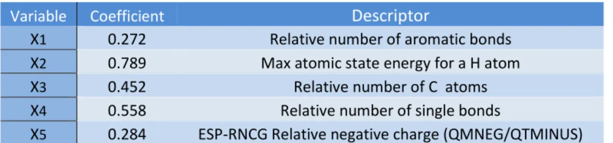
The model with the lowest cost function has test set statistics R

2

train

= 0.8967.

The model has 5 descriptors:

pIC50

= 5.134 + 0.272 X

₁

- 0.789 X

₂

+ 0.452 X

₃

+ 0.558 X

₄

+ 0.284 X

₅

Model performance:

(33)

Variable Coefficient

Descriptor

X1 0.272 Relative number of aromatic bonds

X2 0.789 Max atomic state energy for a H atom

X3 0.452 Relative number of C atoms

X4 0.558 Relative number of single bonds

X5 0.284 ESP-RNCG Relative negative charge (QMNEG/QTMINUS) Table 3: Selected Descriptors in β-Diketo Acid QSAR Model- 91 B-diketo acids (DE-BPSO-MLR)

Based on this QSAR model the descriptors with the highest influence on the biological activity

of aryl B-diketo acids are the Relative number of single bonds and Relative number of C atoms.

Model Accuracy plot:

Figure 11: Results by using DE-BPSO Algorithm and Multiple Linear Regression (DE-BPSO-MLR) for developing QSAR model (91 Aryl B-Diketo Acids)

Comparison of our work with the previous researches:

Since, the DE-BPSO is totally a new hybrid algorithm that has been introduced recently; no

significant work had been done previously using this algorithm. The only earlier research

(34)

available to compare has been on 37 dimeric aryl



-diketo acids acids (Train set =23, Validation

set = 7 and Test set = 7) using Linear Model (MLR) and DE-BPSO algorithm as the feature

selection method (GeneKo,2012). So, we are comparing the result from that research with our

result. The comparison between this work (the data set of 91 dimeric aryl



-diketo acids) and

the previous one (the data set of 37 dimeric aryl



-diketo acids) shows improvement in the

value of R

2

for all the train, validation and test sets.

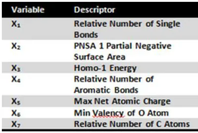
The final QSAR model and R

2

values obtained from previous research are:

pIC50

= 5.134 – 0.360 X1 + 0.628 X2 + 0.619 X3 + 0.157 X4 + 0.242 X5R

2

= 0.886 (n = 23), R

2

v =

0.765 (n = 7), R

2

test= 0.722 (n = 7)

Table 4: Descriptors used in QSAR Model (Data set of 37 β-Diketo Acids)

Based on this QSAR model, hydrophobicity of the compounds (X2) and partial positive charges

on the hydrogen atoms on the molecular surface (X3) have the highest significance in the

biological activities (GeneKo,2012).

However, MLR is a common modelling method for QSAR development, comparing the results of

linear model with Non-Linear Models such as Random Forest will lead to a more accurate

analysis and comparison.

5.2 Results of using Non-linear model: random Forest and TreeNet

Salford System’s RandomForests and TreeNet Predictive Modeling software (Salford Systems)is

used to evaluate our data. Both systems are a decision-tree model that sorts the data to find

the most impactful descriptors.

After running our data set on both the Random Forest and TreeNet systems, two separate

results were obtained. The most interest was in the R

2

value of each model first. For the

Random Forest model, an R

2out-of-bag(test)

value of 0.43 was obtained (testing). This was

(35)

significantly smaller than linear model, DE-BPSO, R

2test

value of 0.8677.The R

2train

value

obtained from TreeNet was 0.648. It has been found that the R

2test

for TreeNet was 0.475.

Because the obtained TreeNet R

2train

value was greater than 0.5, the research proceeded with

formulating the pIC50 with the variables with the highest scores in TreeNet. The following

formula is to represent pIC50 using the TreeNet system. Additionally, the variable importance

descriptors in the pIC50 are shown in Table 5: pIC50 variable importance descriptors used in pIC50

using the TreeNet system, ranked by variable importance score

Table 5: pIC50 variable importance descriptors used in pIC50 using the TreeNet system, ranked by variable importance score

Next, the MSE charts for both the TreeNet (Figure 12: MSE vs. Number of Trees for learning and

testing curves in TreeNet) and Random Forest (Figure 13: MSE vs. Number of Trees for the learning curve in Random Forest) models were generated and evaluated. Figure 12: MSE vs. Number of Trees

for learning and testing curves in TreeNetrepresents the TreeNet model, depicts the learning

graph, which is defined by each individual tree built, and the test line is defined by the

randomly selected data objects used to test each tree’s model. The mean squared error for 200

trees was found to be 0.3457.

In Figure 13: MSE vs. Number of Trees for the learning curve in Random Forest, the Random Forest

MSE for 500 trees was about 0.412

(36)

Figure 12: MSE vs. Number of Trees for learning and testing curves in TreeNet

Figure 13: MSE vs. Number of Trees for the learning curve in Random Forest

Clearly, our linear model (data set of 91 acids) with the help of Evolutionary Algorithm

(DE-BPSO) has shown better results comparing the previous research on linear model (data set of

37 acids). Also, it clearly shows better results than Random Forest and Tree-Net of SPM

provided by the SPM (shown in

Table 6: Comparing Coefficient of Determination

). One reason is

that based on our research we have realized that SPM works much better against large dataset

i

.

So, the algorithm does poorly when we only have a few observations. Another reason is that it

is possible that our data are more appropriate for linear models than none-linear ones.

Data Set Coefficient Of Determination

37 B-aryl -diketo acids (Linear - MLR) 0.886

91 B-aryl-diketo acids ( Linear - MLR) 0.8967

91 B-diketo acids ( NonLinear- RF) 0.434

91 B-diketo acids(NonLinear- TreeNet) 0.648

Table 6: Comparing Coefficient of Determination (Goodness of Fit) for linear and non-linear models

(37)

6. The QSAR Database

6.1 The QSAR Database repository and Web modeling system

The CSUSM QSAR Web Modelling System is designed to be a scalable web application

framework used to train quantitative structure-activity relationship (QSAR) models for purposes

of identifying unique optimal physicochemical properties in bio-pharmaceutical chemical drug

compound data sets.

Figure 14: Architecture

Requirements

The following software components comprise the CSUSM QSAR Web Modelling System.

● Supported Web Browser

○ Internet Explorer 10+, Chrome, FireFox ● Anaconda Python 2.7 by Continuum Analytics

○ Provides the Python language along with core scientific computing libraries ● Django 1.7

(38)

○ Core web application platform

● RabbitMQ

○ Message broker platform used as the modelling system’s core inter-process communication system implementing the Advanced Message Queuing Protocol ● Pika Python-driver for RabbitMQ

○ Python driver to support message passing with RabbitMQ ● Celery 3.1 Distributed Task Queue

○ Distributed worker platform used for run training tasks in parallel ● PostgreSQL 9.3 or greater

○ Relational database platform used as the main data repository for training configuration, input and output data entities.

6.2 Creating the QSAR Database

The CSUSM QSAR Web Modelling System relies on a relational database backend for its session management and model configuration metadata. This platform supports the user-session context persistence workflow and stores both configuration and input and output metadata as entities in a relational-database model. Postgres was chosen due to its stricter adherence to current SQL standards and cross-platform support, both of these among other aspects help make the CSUSM QSAR Web Modelling System a more extendible and cross-platform application

(39)

To create the database that supports the backend of the CSUSM QSAR Web Modelling System, the above Entity Relationship Model (ERD) has been designed and developed. This database consists of six entities, to create the relationship(s) between these entities the efficiency of retrieving all the required information by query on the “Session” entity has been considered.

The result is 6 tables as follows:

● Input (Input_id, Input_File_Loc) ● Output (Output_Id, Output_File_Loc) ● Implementation (Imp_Id, Imp_Desc)

● Evo_Alg (Impl_Id, Evp_Alg_Name, Evo_Alg_Desc)

● Model (Impl_Id, Evp_Alg_Name, Model_Name, Type_Name)

● Session (Session_Id, sessionhash, sessionsalt, Creation_Date, , Input_Id, Output_Id, Impl_Id, Elv_Alg_Name, Model_Name)

6.3 Managing & Working with the QSAR Database

The CSUSM QSAR Web Modelling System provides a convenient interface to its backend database through a common web browser. This interface is accessible using the (optional) administrative account created as part of the Section III setup procedure. The following snapshots show how you can

manipulate entities in the QSAR database.

(40)

After choosing the related database(Qsar), each entity should be added to the database ( by database administrator).

Figure 17: Add any defined Entity type to the QSAR database

Now that the “Models” is a defined entity in the database, the admin can add a new model to the database.

Figure 18: Adding a new (Model) entity to the QSAR Database

After the new model is added ( as a linear or a non linear model ), it will be visible to the user through the Machine Learning Models window.

(41)

Also, it is possible to change, update or delete any model.

Figure 20: Models can be changed, i.e. either updated or deleted

It is possible to authorize multiple administer users, add them or change them through this system.

Figure 21: Additional administrator users can be added or changed from the main dashboard

6.4 Interacting with the QSAR Web Modelling System

The QSAR Web Modelling System uses a standard web browser as its primary user interface. The following sections describe how a user can interact with the system to train a model using an uploaded example data set.

(42)

A. Creating a New Session

Right after connecting to the system, the following page will be visible to the visitor as the first page. On this page the user clicks “Choose Model and Data”

At first the user should choose Machine Learning Model Type, Machine Learning Model, Evolutionary Algorithm and Implementation Method. Two types are supported: linear and non-linear. For the linear model we have currently supported: Multiple Linear Regression (MLR), Support Vector Machine (SVM) and Partial Least Squares Regression (PLSR). For the non-linear models we have currently supported: Random Forest (RF) and Artificial Neural Network (ANN). We have also supported Evolutionary Algorithms such as: Genetic algorithm (GA), Binary Particle Swarm Optimization algorithm(BPSO), Differential Evolution algorithm(DE) and The Hybrid Differential Evolutionary – Binary Particle Swarm Optimization algorithm (DE-BPSO). There are several ways that each algorithm can be implemented and there are several parameters that can be used to make the changes to twist the result in different ways. The last option, “Implementation Methods” helps the users to select how they prefer to execute their models against their data.

Figure 23: Select Model Configuration

(43)

Figure 24: Create Session ID

(44)

B. Uploading External Data

A user has the ability to upload a training set data file. Currently only csv files are supported.

Figure 26: Uploading External Data

C. Starting a Training Session

Once a new data set file has been uploaded for session, a user can start training their configured model

(45)

D. Get Training Status

After training has started, a user can click “Get Training Status” from the main configuration console to retrieve messages about the state of any in-progress model training.

Figure 28: Get Training Status

E. Stopping a Training Session

A user, at any time, has the ability to halt any in-progress model training/

(46)

F. Downloading Training Results

A user may download training results from a successfully completed training model

Figure 30: Downloading Training Status

G. Restoring an Existing Session

A user can also restore their session using a reference to the session’s unique identifier. This makes it convenient and possible for the user to easily restore an active session at any time event when model training is in progress.

(47)

By clicking the “Copy Session ID to Clipboard”, and then paste it as the extension of the current URL The system restores and shows the session ID.

(48)

7. Conclusion and future work

The TreeNet algorithm performed well in searching for a set of descriptors with good statistical

performance. The selected QSAR model for the analysis of β-diketo acids had a correlation of

R

2

= 0.648 and predictive statistics of R

2test

= 0.475 for TreeNet and

R

2outofbag

= 0.43 for Random Forest.

Random Forest’s R

2

was significantly smaller than the linear model, DE-BPSO, which had a

R

test2

value of 0.8098 and R

train2

was 0.8967. In addition, any R

2

value under 0.5 has been

labeled as non-predictive for this research purposes. However, an encouraging value using

TreeNet is found.

The R

2

train

value obtained from TreeNet was 0.648. It is found that the R

2

test

for TreeNet was

0.475. Because the TreeNet R

2

value was greater than 0.5, we proceeded with formulating the

pIC50 with the variables with the highest scores in TreeNet. Based on this model, the

descriptors with the greatest influence on the biological activity of β-diketo acids are those

which are related to molecular volume, topology, and electrostatic effects, with large molecular

volumes having the greatest impact.

The TreeNet model found the two most important features to be a relative number of single

bonds, and a partial negative surface area. This is encouraging because the HIV-1 integrase

active site is considered to be hydrophobic in nature with a single Mg

2+

ion available for

chelation with a drug compound for enzymatic inhibition. The negative charged surface area

descriptors capture the plausibility of electrostatic interactions with the Mg

2+

ion in the active

site (Gonzalez). Because the R

2

Improving HIV-1 Integrase Inhibitors Prediction Using Hybrid Differential Evolution-Binary Particle Swarm Algorithm