A Novel Algorithm for Detecting Protein Complexes with the Breadth First Search

(1)

Georgia State University

ScholarWorks @ Georgia State University

Computer Science Faculty Publications

Department of Computer Science

2014

A Novel Algorithm for Detecting Protein

Complexes with the Breadth First Search

Xiwei Tang

Central South University

Jianxin Wang

Central South University, [email protected]

Min Li

Central South University, [email protected]

Yiming He

Central South University

Yi Pan

Georgia State University, [email protected]

Follow this and additional works at:

http://scholarworks.gsu.edu/computer_science_facpub

Part of the

Computer Sciences Commons

This Article is brought to you for free and open access by the Department of Computer Science at ScholarWorks @ Georgia State University. It has been accepted for inclusion in Computer Science Faculty Publications by an authorized administrator of ScholarWorks @ Georgia State University. For more information, please [email protected].

Recommended Citation

Tang, Xiwei; Wang, Jianxin; Li, Min; He, Yiming; and Pan, Yi, "A Novel Algorithm for Detecting Protein Complexes with the Breadth First Search" (2014).Computer Science Faculty Publications.Paper 24.

(2)

Research Article

A Novel Algorithm for Detecting Protein Complexes with the

Breadth First Search

Xiwei Tang,

1,2

Jianxin Wang,

1

Min Li,

1

Yiming He,

1

and Yi Pan

1,3 1_{School of Information Science and Engineering, Central South University, Changsha 410083, China} 2_{School of Information Science and Engineering, Hunan First Normal University, Changsha 410205, China} 3_{Department of Computer Science, Georgia State University, Atlanta, GA 30302-4110, USA}

Correspondence should be addressed to Jianxin Wang; [email protected] Received 27 January 2014; Accepted 19 March 2014; Published 10 April 2014 Academic Editor: FangXiang Wu

Copyright © 2014 Xiwei Tang et al. This is an open access article distributed under the Creative Commons Attribution License, which permits unrestricted use, distribution, and reproduction in any medium, provided the original work is properly cited. Most biological processes are carried out by protein complexes. A substantial number of false positives of the protein-protein interaction (PPI) data can compromise the utility of the datasets for complexes reconstruction. In order to reduce the impact of such discrepancies, a number of data integration and affinity scoring schemes have been devised. The methods encode the reliabilities (confidence) of physical interactions between pairs of proteins. The challenge now is to identify novel and meaningful protein complexes from the weighted PPI network. To address this problem, a novel protein complex mining algorithm ClusterBFS (Cluster with Breadth-First Search) is proposed. Based on the weighted density, ClusterBFS detects protein complexes of the weighted network by the breadth first search algorithm, which originates from a given seed protein used as starting-point. The experimental results show that ClusterBFS performs significantly better than the other computational approaches in terms of the identification of protein complexes.

1. Introduction

Protein complexes are molecular aggregations of proteins assembled by multiple protein-protein interactions. Many proteins are functional only after they are assembled into a protein complex and interact with other proteins in this complex [1–4]. The vast amount of genes and proteins that participate in biological networks imposes the need for determination of protein complexes within the network in order to reduce the complexity, while these complexes will be the first step in deciphering the composite genetic or cellular interactions of the overall network.

High-throughput experimental technologies, along with computational predictions, have produced a large amount of protein interactions [5–11], which make it possible to uncover protein complexes from protein-protein interaction (PPI) networks. Pair-wise protein interactions can be modeled as a graph or network, where vertices represent proteins and edges are protein-protein interactions. Protein complexes are groups of proteins that interact with one another, so they generally correspond to dense subgraphs in PPI networks.

Different research groups have developed a wealth of algo-rithms to identify protein complexes from the PPI networks [12–18]. In these approaches, the protein networks are con-sidered as unweighted graphs. These methods work well on PPI networks and extract successfully protein complexes. Nevertheless, it has been noticed that protein interaction data produced by high-throughput experiments are often associated with high false positive rate and false negative rate due to the limitations of the associated experimental techniques, which may have a negative impact on the complex discovery algorithms [19–23].

In order to address that particular question, a number of data integration and affinity scoring schemes have been devised [10, 23–30]. In the paper of Gavin et al. [11], the weights of the interactions were defined by using the so-called socio-affinity index introduced in [11] that is based on the log-odds of the number of times two proteins were observed together in a purification, relative to the expected frequency of such a cooccurrence based on the number of times the proteins appeared in purifications. Krogan et al. [10] have used MALDI-TOF mass spectrometry and LC-MS/MS

Volume 2014, Article ID 354539, 8 pages http://dx.doi.org/10.1155/2014/354539

(3)

2 BioMed Research International

to identify protein-protein interactions, based on the obser-vation that either mass spectrometry method often fails to identify a protein, and the usage of two independent methods can increase the coverage and confidence of the obtained interactome. The results of the two methods were combined by supervised machine learning methods with two rounds of learning, using hand-curated protein complexes in the MIPS reference database as a gold standard dataset. Collins et al. [23] have combined the experimentally derived PPI networks of Krogan et al. [10] and Gavin et al. [11] by re-analyzing the raw primary affinity purification data of these experiments using a novel scoring technique called purification enrich-ment (PE). The PE scores were motivated by the probabilistic socio-affinity scoring framework of Gavin et al. [11] but also take into account negative evidence (i.e., pairs of proteins where one of them fails to appear as a prey when the other one is used as a bait). These affinity scores encode the reliabilities (confidence) of physical interactions between pairs of pro-teins. Therefore, the challenge now is to mine meaningful and novel complexes from protein interaction networks derived by combining multiple high-throughput datasets and by making use of these affinity scoring schemes. In this direc-tion, some algorithms have also been proposed [25,31–34].

In this study, we propose a novel algorithm to derive yeast complexes from weighted (affinity-scored) PPI network and call it ClusterBFS (Cluster with Breadth First Search). ClusterBFS builds clusters in terms of breadth first search algorithm, starting from local seeds and adding nodes that maintain the weighted density of the clusters. The experi-mental results show that our ClusterBFS method outperforms existing computational methods, such as MCL [31], Clus-terONE [32], HC-PIN [33], SPICi [34], and MCODE [14].

2. Methods

2.1. Preliminaries. Given a weighted network, the goal of our algorithm is to output a set of disjoint dense subgraphs. We model the network as a undirected graph𝐺 = (𝑉, 𝐸)with a confidence score0 < 𝑤_𝑢,V ≤ 1, for every edge(𝑢,V) ∈ 𝐸. For any two vertices,𝑢andVwithout an edge between them, we set𝑤_𝑢,V = 0. For each set of vertices𝑆 ⊂ 𝐸, we define its weighted density as the sum of the weights of the edges among them divided by the total number of possible edges (i.e., the density of a set is measure of how close the induced subgraph is to clique, and varies from 0 to 1):

𝐷_𝑤(𝑆) = _{|𝑆| ∗ (|𝑆| − 1) /2}∑(𝑢,V)∈𝑆𝑤𝑢,V . (1)

2.2. Algorithm Overview. We use a breadth first search approach to build clusters. ClusterBFS builds one cluster at a time, and each cluster is expanded from an original seed protein. The unclustered node is added, if it has the highest edge weight and the density of the cluster remains higher than a user-defined threshold Td; otherwise, the cluster is output. The growth process is repeated from different seeds to form multiple, possibly, overlapping groups. Although some overlaps are likely to have biological importance, groups overlapping to a very high extent in comparison to their

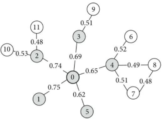
9 6 8 4 7 0 3 2 11 10 1 5 0.75 0.62 0.51 0.48 0.49 0.52 0.65 0.69 0.74 0.48 0.53 0.51

Figure 1: Example to illustrate the clustering process. This example network has 12 vertices, and every edge has confidence. Suppose the weighted density threshold𝑇𝑑 = 0.2. The vertex 0 is taken as a seed protein and the original cluster 0 is constructed. In the first step of the breadth first search, the vertex 1 has the highest edge weight 0.75 among the neighbors of the vertex 0. We add vertex 1 to the cluster and this cluster{0, 1}now has the weighted density 0.75 that is bigger than the density threshold 0.2. Similarly, the vertices 2, 3, 4, and 5 are added to the cluster in sequence and the cluster{0, 1, 2, 3, 4, 5} now has the weighted density 0.23 which is still more than the threshold 0.2. Next, the neighbors of vertex 4 are considered. Of these, vertex 6 has the highest edge weight 0.52 and is added to the cluster. However, the weighted density of the cluster{0, 1, 2, 3, 4, 5, 6} is 0.19 and less than the threshold 0.2. Thus, the vertex 6 is removed and the neighbor of the vertex 3 is examined. Because the weighted value between the vertex 3 and its neighboring vertex 9 is 0.51 and less than 0.52, the vertex 9 is not added to the cluster. When the neighbors of the vertex 2 are checked, the vertex 10 is added to the cluster. Since the weighted density of the cluster{0, 1, 2, 3, 4, 5, 10} is less than 0.2, the vertex 10 is removed. And, likewise, the vertex 11 is not added to the cluster. We stop extending the cluster and output the final cluster{0, 1, 2, 3, 4, 5}. For simplicity, the elimination of redundant clusters is not shown in this figure.

sizes should likely be discarded. We quantify the extent of overlap between each pair of groups and discard the smaller group, if the overlap score [14] is above a specified threshold. ClusterBFS thus has two parameters:Td, the weighted density threshold and𝑅. For threshold𝑅, we set a firm value 0.8 [32]. (SeeFigure 1for a simplified example.)

2.3. Seed Selection. Every vertex in the yeast PPI network is used as the seed and is equally important.

2.4. Cluster Expansion. After obtaining the seed vertex, we use the breadth first search method to grow each cluster in terms of the weighted density. At each step, we have a current vertex set𝐶for the cluster, which initially contains one seed proteinV. We search for the vertex𝑢with maximum value of the edge weight amongst all the unclustered vertices that are adjacent to the seed Vin breadth first. If the weighted density of the cluster is smaller than a threshold, we stop expanding this cluster and output it. If not, we put vertex𝑢 into𝐶and update the density value. If the density value is smaller than our density thresholdTd, we do not include𝑢in the cluster and output𝐶. We repeat this procedure until all vertices in the graph are clustered.Algorithm 1illustrates the

(4)

Input:

weighted PPI network𝐺 = (𝑉, 𝐸_𝑤); weighted density threshold𝑇𝑑; overlap score threshold𝑅;

Output:

set of protein complexes SC discovered from𝐺;

Description:

(1) SC= 𝜙;//initialization (2) for each vertexV∈ 𝑉do

(3) construct the complex,𝐶 =BFS(𝐺,V);

//𝐷_𝑤(𝐶) > 𝑇𝑑

(4) 𝑉 = 𝑉 − {V};

(5) Redundancy-filtering (𝐶);

Algorithm 1: ClusterBFS algorithm.

(1)𝑟𝑒𝑠𝑢𝑙𝑡𝑠 =V

(2) create a queue𝑄

(3)𝑄 = {V_𝑖|V_𝑖∈ 𝑉 ∩ 𝑑𝑖𝑠(V, V_𝑖) = 1}

(4) while𝑄is not empty: (5) begin (6) 𝑡 ← 𝑄.𝑑𝑒𝑞𝑢𝑒𝑢𝑒() (7) 𝑟𝑒𝑠𝑢𝑙𝑡𝑠 = 𝑟𝑒𝑠𝑢𝑙𝑡𝑠 ∪ {𝑡} (8) if𝐷_𝑤(𝑟𝑒𝑠𝑢𝑙𝑡𝑠) ≤ 𝑇𝑑: (9) 𝑟𝑒𝑠𝑢𝑙𝑡𝑠 = 𝑟𝑒𝑠𝑢𝑙𝑡𝑠 − {𝑡} (10) else (11) 𝑄 = 𝑄 ∪ {V_𝑖|V_𝑖∈ 𝑉 ∩ 𝑑𝑖𝑠(𝑡, V_𝑖) = 1} (12) end (13) return results

Algorithm 2: Breadth First Search: BFS(𝐺,V).

over framework to detect protein complexes.Algorithm 2is the breadth first search procedure.

Since all vertices in the graph have been selected as seeds, the clusters produced have large overlaps, which will result in high redundancy. Hence, a Redundancy-filtering procedure is designed to process candidate clusters and finally generate protein complexes by eliminating such kind of redundancy.Algorithm 3shows details of the redundancy process. Suppose that SC is the set of all currently detected complexes and𝐶 = (𝑉_𝐶, 𝐸_𝐶)is a newly identified complex. We will first selected an element𝐵 = (𝑉_𝐵, 𝐸_𝐵)in SC, which has the highest similarity (OS, overlap score) [14] with𝐶. In

Algorithm 3, the procedure Redundancy-filtering (𝐶) is used to check and decide whether to discard or preserve the newly selected Complex𝐶. If𝐵and𝐶are not quite similar (with

OS < 𝑅),𝐶will be inserted into SC in lines 2-3; otherwise,

we prefer to preserve the complexes that have larger size in lines 4–8. For instance, suppose Complex 𝐵of Figure 2 is one complex belonging to the complex set SC and is the most similar to the new complex, that is, Complex𝐶. After computing the OS of the two complexes, we obtain a score 0.11 which is less than the threshold𝑅 = 0.8. So Complex𝐶 will be inserted into the complex set SC.

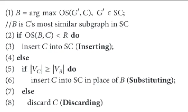
(1)𝐵 =arg max OS(𝐺󸀠, 𝐶), 𝐺󸀠∈SC;

//𝐵is𝐶’s most similar subgraph in SC (2) if OS(𝐵, 𝐶) < 𝑅do

(3) insert𝐶into SC (Inserting); (4) else

(5) if 󵄨󵄨󵄨󵄨𝑉_𝐶󵄨󵄨󵄨󵄨 ≥ 󵄨󵄨󵄨󵄨𝑉_𝐵󵄨󵄨󵄨󵄨do

(6) insert𝐶into SC in place of𝐵(Substituting); (7) else (8) discard𝐶(Discarding) Algorithm 3: Redundancy-filtering (𝐶). Complex C Complex B A A B B C C D D E F G H I J K L M _N O P Q T S R

Figure 2: Example to illustrate the Redundancy-filtering. Complex

𝐵and Complex𝐶contain 14 and 10 proteins, respectively. They share 4 proteins A, B, C, and D.

3. Results

We test the performance of our ClusterBFS method with other five competing algorithms, Markov cluster (MCL) [31], clustering with overlapping neighborhood expansion (Clus-terONE) [32], hierarchical clustering on protein interaction network (HC-PIN) [33], speed and performance in clustering (SPICi) [34], and molecular complex detection (MCODE) [14] using the weighted Collins [23] and Krogan datasets [10]. For each algorithm, the final results are obtained after having optimized the algorithm parameters to yield the best possible results. We compare predicted complexes to the reference complex set CYC2008 [35]. We assess the quality of the predicted complexes by two scores: the fraction of protein complexes matched by at least one predicted complex and the maximum matching ratio (MMR) [32]. Our benchmarks show that ClusterBFS outperforms the other approaches on weighted networks, matching more complexes with a higher𝐹-measure and providing a better one-to-one map-ping with reference complexes in three datasets. To examine the biological relevant of detected complexes we calculate the colocalization and coannotation scores of the entire identified complex set [24]. Comparison of colocalization and coannotation scores of ClusterBFS complexes and other algorithms reveals that ClusterBFS has higher scores on three datasets.

(5)

3.1. Data Sources. Yeast has long been known as a highly effective model organism for mammalian biological func-tions and diseases. We evaluate the effectiveness of Clus-terBFS using three different yeast PPI weighted networks. The first dataset is prepared by Collins et al. [23]. For the weighted interaction map of Collins et al., we use the top 9074 interactions as suggested by the authors. These interactions among 1622 proteins have very high confidence scores. The second dataset is the Krogan core dataset [10]. It consists of 7123 reliable interactions involving 2708 proteins. We also use Krogan’s extended dataset [10] containing 3672 nodes and 14317 edges to test ClusterBFS. For evaluating our identified complexes, the set of real complexes from [35] is selected as benchmark.

3.2. Evaluation Measures. One evaluation method we use is to match the generated complexes with known complex set [35] and calculate sensitivity, positive predictive value (PPV),

𝐹-measure, and MMR, respectively. In information retrieval, positive predictive value is called precision, and sensitivity is called recall. We derive 408 typical complexes including two or more proteins from the CYC2008 [35] as the benchmark complex set and use the same scoring scheme used by [14] to determine how effectively a predicted complex matches a reference complex. If two complexes overlap each other, they must share one or more proteins. The overlap score (OS) of a predicted complex versus a benchmark complex is then a measure of biological significance of the prediction, assuming that the benchmark set of complexes is biologically relevant. The overlap score between a predicted and a real complex is calculated using

OS= 𝑖

2

𝑔 × ℎ, (2)

where𝑖refers to the number of proteins shared by a predicted complex and a benchmark complex, 𝑔 is the number of proteins in the predicted complex, andℎis the number of proteins in the benchmark complex. If OS is 1, it means that a complex has the same proteins as a benchmark complex. On the contrary, when OS is more than 0, there is not a shared protein between the predicted complex and the benchmark complex [14].

The number of true positives (TP) is defined as the num-ber of predicted complexes with OS over a threshold value and the number of false positives (FP) is the total number of predicted complexes minus TP. The number of false negatives (FN) equals the number of known complexes not matched by predicted complexes. 𝑅𝑒𝑐𝑎𝑙𝑙 and 𝑃𝑟𝑒𝑐𝑖𝑠𝑖𝑜𝑛 are defined as TP/(TP + FN) and TP/(TP + FP), respectively [14]. 𝐹 -measure, or the harmonic mean of 𝑅𝑒𝑐𝑎𝑙𝑙 and 𝑃𝑟𝑒𝑐𝑖𝑠𝑖𝑜𝑛, can then be used to evaluate the overall performance of the clustering algorithms:

𝐹-measure=2 × 𝑅𝑒𝑐𝑎𝑙𝑙 × 𝑃𝑟𝑒𝑐𝑖𝑠𝑖𝑜𝑛

𝑅𝑒𝑐𝑎𝑙𝑙 + 𝑃𝑟𝑒𝑐𝑖𝑠𝑖𝑜𝑛 . (3)

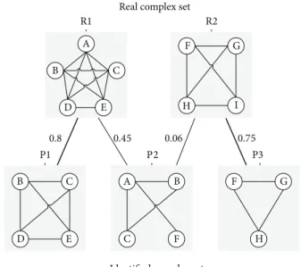
MMR score is proposed by Nepusz et al. [32] based on a maximal one-to-one mapping between detected and refer-ence complexes.Figure 3illustrates the maximum matching ratio.

Real complex set

R1 A _F _G B C D D E H I 0.8 0.45 0.06 0.75 P1 P3 C A B B F G E C F H Identified complex set

P2

R2

Figure 3: Example to illustrate the maximum matching ratio. R1 and R2 are real complexes, while P1, P2, and P3 are three predictions. An edge connects a reference complex and a predicted complex, if their overlap score is larger than zero. The maximum matching is shown by the thick edges. Note that P2 was not matched to R1 since P1 provides a better match with R1. The maximum matching ratio in this example is (0.8 + 0.75)/2 = 0.775.

Owing to the fact that gold standard protein complex sets are incomplete [36], a predicted complex that does not match any of the reference complexes may belong to a valid but previously uncharacterized complex as well. To this end, the matching measures should be complemented with scores that assess the biological relevance of predicted complexes based on the colocalization and coannotation of the constituent proteins instead of relying on a predefined gold standard. Since protein complexes are formed to perform a specific cellular function, proteins within the same complex tend to share common functions and be colocalized [37]. Generally, higher coannotation and colocalization scores [24] show that proteins within the same protein complexes tend to share higher functional similarity. We employ the software suite ProCope (http://www.bio.ifi.lmu.de/Complexes/ProCope/) to compute the colocalization and coannotation scores in our experiment.

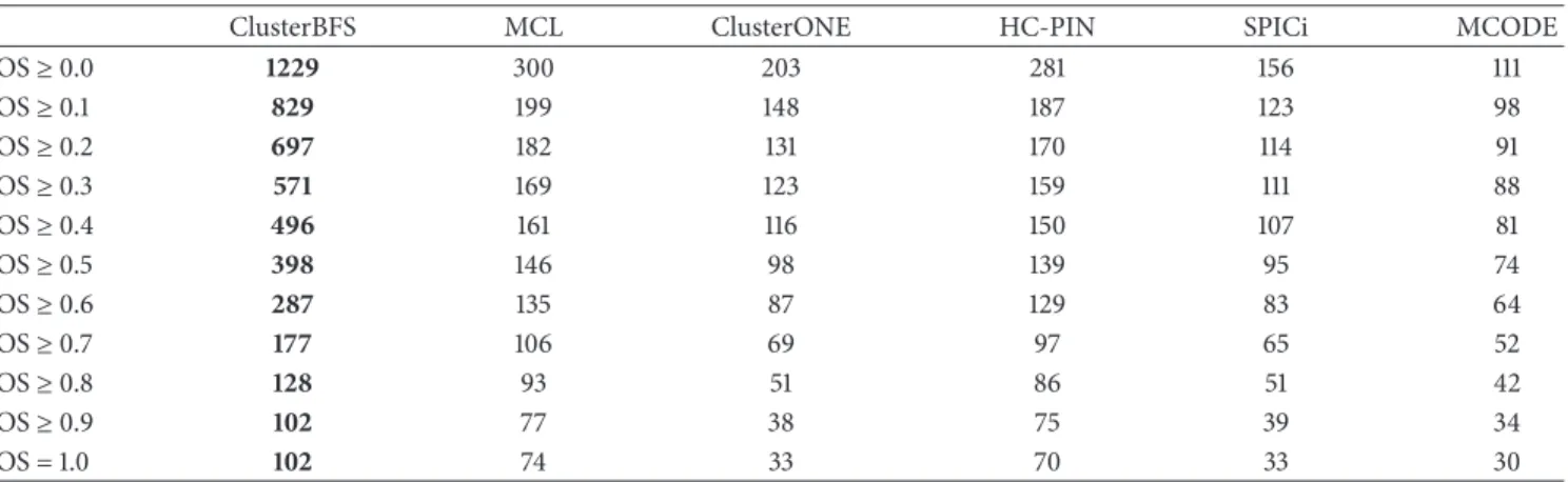
3.3. Comparison with the Real Complexes on the Collins Dataset. Table 1 shows the number of detected complexes that match at least one real complex over a range of OS thresholds from threshold of 0 to 1.0 (in 0.1 increments). From

Table 1, it can be found that the ClusterBFS algorithm detects the most complexes which match at least one known complex over every interval of OS. The second line inTable 1shows the number of all complexes discovered by each approach. For instance, ClusterBFS predicts altogether 1229 complexes from the Collins dataset, whereas MCL, ClusterONE, HC-PIN, SPICi, and MCODE find 300, 203, 281, 156, and 111 complexes, respectively. The third line displays that when OS is more than 0.1, ClusterBFS curates 829 complexes matched at least

(6)

Table 1: Comparison of the number of predictions matching at least one known complex.

ClusterBFS MCL ClusterONE HC-PIN SPICi MCODE

OS≥0.0 1229 300 203 281 156 111 OS≥0.1 829 199 148 187 123 98 OS≥0.2 697 182 131 170 114 91 OS≥0.3 571 169 123 159 111 88 OS≥0.4 496 161 116 150 107 81 OS≥0.5 398 146 98 139 95 74 OS≥0.6 287 135 87 129 83 64 OS≥0.7 177 106 69 97 65 52 OS≥0.8 128 93 51 86 51 42 OS≥0.9 102 77 38 75 39 34 OS = 1.0 102 74 33 70 33 30

Table 2: Comparison of the number of real complexes matching at least one detected complex.

ClusterBFS MCL ClusterONE HC-PIN SPICi MCODE

OS≥0.0 408 408 408 408 408 408 OS≥0.1 298 256 195 244 176 142 OS≥0.2 269 227 164 209 142 113 OS≥0.3 239 196 149 185 129 103 OS≥0.4 224 181 137 171 117 92 OS≥0.5 206 159 111 150 104 82 OS≥0.6 181 145 96 136 88 70 OS≥0.7 133 109 73 100 68 54 OS≥0.8 115 94 52 87 53 42 OS≥0.9 102 77 38 75 39 34 OS = 1.0 102 74 33 70 33 30

one real complex but MCL, ClusterONE, HC-PIN, SPICi, and MCODE merely mine 199, 148, 187, 123, and 98 complexes like that, respectively.Table 2gives the number of real complexes which match at least a predicted one. Table 2 shows that the number of real complexes matched by predicted ones from ClusterBFS is also the largest. The experimental results demonstrate that although ClusterBFS obtains the largest number of complexes, the matched complexes from Clus-terBFS are much more than those from the other techniques. That is, ClusterBFS identifies a vast amount of high-quality complexes from the weighted Collins network.

In addition, as shown in Tables 1 and 2, when OS is 1, ClusterBFS identifies 102 real complexes. In other words, 102 predicted complexes from ClusterBFS also belong to the known complex set [35] and are much more than ones from one of the other approaches including MCL, ClusterONE, HC-PIN, SPICi, and MCODE, respectively. More importantly, we observe that the reference set includes 408 real complexes, of which 259 complexes are the small size complex only containing 2 or 3 proteins. Actually, our statistical results (not presented in the tables of the paper) show that, in the 102 real complexes predicted by ClusterBFS, there are 78 small size complexes like that. However, MCL, HC-PIN, SPICi, and MCODE only find 74, 70, 33, and 30 real complexes, respectively. At the same time, MCL, HC-PIN, SPICi, and MCODE just detect 54, 49, 15, and 9 small

size real complexes. Since ClusterONE discards the complex candidates that contain less than three proteins, we do not compare it with ClusterBFS. The experimental results show that ClusterBFS has the significant performance advantage over the other algorithms in terms of the identification of small size complexes.

Next, we calculate the𝐹-measure and MMR scores of the complex sets detected by various techniques. When the𝐹 -measure is computed, the OS between a predicted complex and a real complex in the benchmark is set as 0.2 [14].

Figure 4 displays the overall comparison according to 𝐹 -measure and MMR. On Collins dataset, the 𝐹-measure of ClusterBFS is 0.68, which is 23.6%, 51.1%, 30.8%, 58.1%, and 83.8% higher than MCL, ClusterONE, HC-PIN, SPICi, and MCODE, respectively. ClusterBFS can achieve the highest𝐹 -measure, which shows that our method can predict protein complexes very accurately. FromFigure 4, it also can be found that our ClusterBFS method obtains the highest MMR of 0.64, which is 21.8%, 33.3%, 21.8%, 25.5%, and 36.2% higher than MCL, ClusterONE, HC-PIN, SPICi, and MCODE, respectively. That is, ClusterBFS provides a better one-to-one mapping with real complexes in the Collins dataset.

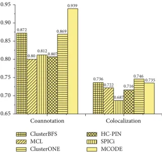
3.4. Biological Coherence of Predicted Complexes on Collins Dataset. Figure 5shows the colocalization and coannotation scores of complexes detected by various methods. From

(7)

6 BioMed Research International ClusterBFS MCL 0.70 _0.68 ClusterONE HC-PIN 0.64 0.65 SPICi MCODE 0.60 0.55 0.55 _0.52 0.53 0.53 0.51 0.50 _0.48 _0.47 0.45 0.45 0.43 0.40 0.37 0.35 0.30 F-measure MMR

Figure 4: The 𝐹-measure and MMR of various algorithms on Collins dataset. ClusterBFS MCL ClusterONE HC-PIN SPICi MCODE 0.95 0.939 0.90 0.872 _0.869 0.85 0.812 0.80 0.80 0.807 0.75 0.736 0.7460.735 0.722 0.716 0.70 0.687 0.65 Coannotation Colocalization

Figure 5: Co-localization and co-annotation scores of complexes identified by various methods on Collins dataset.

Figure 5, it can be observed that ClusterBFS has the second highest colocalization score in the five methods after SPICi. However, SPICi cannot handle overlaps. Proteins may have multiple functions, and therefore the corresponding nodes may belong to more than one cluster; for example, 207 of 1,628 proteins in the CYC2008 hand-curated yeast complex dataset [35] participate in more than one complex. So it is important to detect the overlapping complexes. In addition, it can be seen that the coannotation score of ClusterBFS is lower than that of MCODE. It means that the complexes mined by MCODE have the highest biological significance. How-ever, the disadvantage of MCODE is that it only discovers 111 complexes. In other words, the high-quality complexes identified by MCODE are not too many. In terms of the

ClusterBFS MCL ClusterONE HC-PIN SPICi MCODE 0.53 0.54 0.52 0.50 0.50 0.48 0.45 0.46 0.43 0.44 _0.42 _0.42 _0.42 0.42 0.40 0.40 0.39 _0.38 0.38 0.36 0.34 0.32 0.29 0.30 0.28 0.26 0.24 _0.22 0.22 0.20 F-measure MMR

Figure 6:𝐹-measure and MMR of various methods for Krogan’s core dataset.

coannotation and colocalization, the complexes predicted by our ClusterBFS method are observed to have comparable quality with those predicted by SPICi and MCODE but much better than those predicted by MCL, ClusterONE, and HC-PIN.

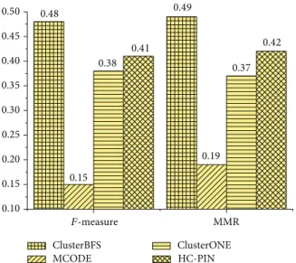
3.5. Results Using Krogan Dataset. To support the credibility of our method, we perform our ClusterBFS on Krogan’s core dataset [10]. The𝐹-measure and MMR of each method using this data are shown in Figure 6. The 𝐹-measure of our ClusterBFS is 0.50, which is 25.0%, 19.0%, 28.2%, 19.0%, and 127.3% higher than MCL, ClusterONE, HC-PIN, SPICi, and MCODE, respectively. From the perspective of MMR, ClusterBFS obtains the score 0.53, which is 39.5%, 23.2%, 26.2%, 17.8%, and 82.76%higher than MCL, ClusterONE, HC-PIN, SPICi, and MCODE, respectively. Additionally, we also test the biological coherence on Krogan’s core data and gain the results which are similar to ones from Collins data. For simplicity, the results are not shown in the paper. In order to evaluate whether ClusterBFS can apply to the larger scale dataset, we test it on Krogan’s extended dataset. The results are shown inFigure 7. FromFigure 7, it can be found that ClusterBFS still obtains the highest scores of𝐹-measure and MMR. The experimental results demonstrate that ClusterBFS is not dependent to a particular kind of dataset and can run well on the larger dataset. Besides, it takes around 1 second on an IBM PC with 3.19 GHz processor and 2 GB RAM to generate clusters from Krogan’s extended dataset.

3.6. Effect of the Parameter Td. In this experiment, we study the effect of the thresholdsTdand𝑅on the performance of ClusterBFS. Nepusz et al. have merged pairs of complexes with an overlap score OS larger 0.8 [32]. So we also set the parameter𝑅0.8 in order to investigate the performance of ClusterBFS under different Td values. Figure 8 shows the 𝐹-measure of ClusterBFS under different values of Td

(8)

ClusterBFS ClusterONE HC-PIN MCODE 0.50 0.48 0.49 0.45 _0.42 0.41 0.40 _0.38 0.37 0.35 0.30 0.25 0.19 0.20 0.15 0.15 0.10 F-measure MMR

Figure 7:𝐹-measure and MMR of various methods for Krogan’s extended dataset. F-measure 0.68 0.67 0.66 0.65 0.64 0.63 0.62 0.61 0.60 0.02 0.04 0.06 0.08 0.10 0.12 0.14 0.16 0.18 0.20 0.22 Td

Figure 8: The effect of parameter Td. Figure 8 shows how the variation of parameterTdaffects the𝐹-measure of ClusterBFS.

based Collins dataset. As shown in Figure 8, when 0.01 ≤ Td≤0.22, the𝐹-measure score of ClusterBFS is more than 0.6 and much higher than those of the other algorithms (SeeFigure 4). Besides, Figure 8also shows that when𝑇 ∈

[0.09, 0.11], ClusterBFS gets the highest 𝐹-measure score.

In this interval, the 𝐹-measure score remains unchanged. Therefore, the parameterTdis set as 0.1 in our experiment.

4. Conclusion

Protein complexes are important for understanding princi-ples of cellular organization and function. Therefore, much work has been concerned with the prediction of protein complexes from the PPI networks. However, the PPI datasets from high-throughput techniques are flooded with false interactions. In response, some research groups propose a

number of data integration and affinity scoring schemes and construct various weighted networks.

In this research, we devise a novel algorithm called ClusterBFS to identify protein complexes from the weighted PPI networks. ClusterBFS derives from the breadth first search method and constitutes protein complexes that orig-inate from a protein seed based on the weighted density. In order to characterize these clusters as protein complexes, we check their biological relevance. This is achieved through some criteria such as𝐹-measure, MMR, colocalization, and coannotation measures. The evaluation of our predictions demonstrates the following advantages of ClusterBFS over the compared approaches. First, ClusterBFS has achieved significantly higher𝐹-measure and MMR than the existing methods. Thus, our predicted complexes match very well with benchmark complexes. Second, ClusterBFS also performs very well in terms of other measures such as coannotation and colocalization, indicating that ClusterBFS can predict protein complexes very accurately. Last but not least, as mentioned above, the real complex set CYC2008 contains a lot of small complexes and so it is necessary to mine them. In comparison with the other approaches, ClusterBFS discovers much more small size complexes. Our identified complexes, therefore, could be probably the true complexes to help the biologists to get novel biological insights.

Conflict of Interests

The authors declare that there is no conflict of interests regarding the publication of the paper.

Acknowledgments

This work is supported in part by the National Natural Science Foundation of China under Grant nos. 61232001, 61370024, and 61379108, the Program for New Century Excellent Talents in University (NCET-12-0547), the Hunan Provincial Natural Science Foundation of China nos. 13JJ6086 and 12JJ6056, and the Hunan Provincial Soft Science Major Program of China no. 2013ZK2014.

References

[1] R. Sharan, I. Ulitsky, and R. Shamir, “Network-based prediction of protein function,”Molecular Systems Biology, vol. 3, pp. 1–13, 2007.

[2] A. D. King, N. Prˇzulj, and I. Jurisica, “Protein complex predic-tion via cost-based clustering,”Bioinformatics, vol. 20, no. 17, pp. 3013–3020, 2004.

[3] C. von Mering, R. Krause, B. Snel et al., “Comparative assess-ment of large-scale data sets of protein-protein interactions,”

Nature, vol. 417, no. 6887, pp. 399–403, 2002.

[4] J. Wang, X. Peng, M. Li, and Y. Pan, “Construction and application of dynamic protein interaction network based on time course gene expression data,”Proteomics, vol. 13, no. 2, pp. 301–312, 2013.

[5] T. Ito, T. Chiba, R. Ozawa, M. Yoshida, M. Hattori, and Y. Sakaki, “A comprehensive two-hybrid analysis to explore the yeast protein interactome,”Proceedings of the National Academy

(9)

of Sciences of the United States of America, vol. 98, no. 8, pp. 4569–4574, 2001.

[6] O. Puig, F. Caspary, G. Rigaut et al., “The tandem affinity purification (TAP) method: a general procedure of protein complex purification,”Methods, vol. 24, no. 3, pp. 218–229, 2001. [7] Y. Ho, A. Gruhler, A. Heilbut et al., “Systematic identification of protein complexes in Saccharomyces cerevisiae by mass spectrometry,”Nature, vol. 415, no. 6868, pp. 180–183, 2002. [8] M. Schena, D. Shalon, R. W. Davis, and P. O. Brown,

“Quantita-tive monitoring of gene expression patterns with a complemen-tary DNA microarray,”Science, vol. 270, no. 5235, pp. 467–470, 1995.

[9] G. Ramsay, “DNA chips: state-of-the art,”Nature Biotechnology, vol. 16, no. 1, pp. 40–44, 1998.

[10] N. J. Krogan, G. Cagney, H. Yu et al., “Global landscape of protein complexes in the yeastSaccharomyces cerevisiae,”

Nature, vol. 440, no. 7084, pp. 637–643, 2006.

[11] A.-C. Gavin, P. Aloy, P. Grandi et al., “Proteome survey reveals modularity of the yeast cell machinery,”Nature, vol. 440, no. 7084, pp. 631–636, 2006.

[12] V. Spirin and L. A. Mirny, “Protein complexes and functional modules in molecular networks,”Proceedings of the National Academy of Sciences of the United States of America, vol. 100, no. 21, pp. 12123–12128, 2003.

[13] G. Palla, I. Der´enyi, I. Farkas, and T. Vicsek, “Uncovering the overlapping community structure of complex networks in nature and society,”Nature, vol. 435, no. 7043, pp. 814–818, 2005. [14] G. D. Bader and C. W. V. Hogue, “An automated method for finding molecular complexes in large protein interaction networks,”BMC Bioinformatics, vol. 4, no. 1, p. 2, 2003. [15] J. Wang, P. Tan, J. Yao, Q. Feng, and J. Chen, “On the minimum

link-length rectilinear spanning path problem: complexity and algorithms,”IEEE Transactions on Computers, 2014.

[16] M. Wu, X. Li, C.-K. Kwoh, and S.-K. Ng, “A core-attachment based method to detect protein complexes in PPI networks,”

BMC Bioinformatics, vol. 10, no. 1, article 169, 2009.

[17] X. Ding, W. Wang, X. Peng, and J. Wang, “Mining protein complexes from PPI networks using the minimum vertex cut,”

Tsinghua Science and Technology, vol. 17, no. 6, pp. 674–681, 2012. [18] B. Zhao, J. Wang, M. Li, F. Wu, and Y. Pan, “Detecting protein complex based on uncertain graph model,”IEEE/ACM Transac-tions on Computational Biology and Bioinformatics, 2013. [19] E. Sprinzak, S. Sattath, and H. Margalit, “How reliable are

exper-imental protein-protein interaction data?”Journal of Molecular Biology, vol. 327, no. 5, pp. 919–923, 2003.

[20] J. Chen and B. Yuan, “Detecting functional modules in the yeast protein-protein interaction network,”Bioinformatics, vol. 22, no. 18, pp. 2283–2290, 2006.

[21] G. D. Bader and C. W. V. Hogue, “Analyzing yeast protein-protein interaction data obtained from different sources,”

Nature Biotechnology, vol. 20, no. 10, pp. 991–997, 2002. [22] N. N. Batada, L. D. Hurst, and M. Tyers, “Evolutionary and

physiological importance of hub proteins,”PLoS Computational Biology, vol. 2, article e88, 2006.

[23] S. R. Collins, P. Kemmeren, X.-C. Zhao et al., “Toward a com-prehensive atlas of the physical interactome of Saccharomyces cerevisiae,”Molecular and Cellular Proteomics, vol. 6, no. 3, pp. 439–450, 2007.

[24] C. C. Friedel, J. Krumsiek, and R. Zimmer, “Bootstrapping the interactome: unsupervised identification of protein complexes

in yeast,”Journal of Computational Biology, vol. 16, no. 8, pp. 971–987, 2009.

[25] X. Tang, Q. Feng, J. Wang, Y. He, and Y. Pan, “Clustering based on multiple biological information: approach for predicting protein complexes,”IET Systems Biology, vol. 7, no. 5, pp. 223– 230, 2013.

[26] M. Wu, Z. Xie, X. Li, C. K. Kwoh, and J. Zheng, “Identifying pro-tein complexes from heterogeneous biological data,”Proteins: Structure, Function, and Bioinformatics, vol. 81, no. 11, pp. 2023– 2033, 2013.

[27] X. Tang, J. Wang, J. Zhong, and Y. Pan, “Predicting essen-tial proteins based on weighted degree centrality,”IEEE/ACM Transactions on Computational Biology and Bioinformatics, 2014.

[28] M. Li, R. Zheng, H. Zhang, J. Wang, and Y. Pan, “Effective identification of essential proteins based on priori knowledge, network topology and gene expressions,”Methods, 2014. [29] W. Kim, “Prediction of essential proteins using topological

properties in GO-pruned PPI network based on machine learning methods,”Tsinghua Science and Technology, vol. 17, no. 6, pp. 645–658, 2012.

[30] G. Liu, L. Wong, and H. N. Chua, “Complex discovery from weighted PPI networks,”Bioinformatics, vol. 25, no. 15, pp. 1891– 1897, 2009.

[31] A. J. Enright, S. van Dongen, and C. A. Ouzounis, “An efficient algorithm for large-scale detection of protein families,”Nucleic Acids Research, vol. 30, no. 7, pp. 1575–1584, 2002.

[32] T. Nepusz, H. Yu, and A. Paccanaro, “Detecting overlapping protein complexes in protein-protein interaction networks,”

Nature Methods, vol. 9, no. 5, pp. 471–472, 2012.

[33] J. Wang, M. Li, J. Chen, and Y. Pan, “A fast hierarchical clustering algorithm for functional modules discovery in protein inter-action networks,”IEEE/ACM Transactions on Computational Biology and Bioinformatics, vol. 8, no. 3, pp. 607–620, 2011. [34] P. Jiang and M. Singh, “SPICi: a fast clustering algorithm for

large biological networks,”Bioinformatics, vol. 26, no. 8, pp. 1105–1111, 2010.

[35] S. Pu, J. Wong, B. Turner, E. Cho, and S. J. Wodak, “Up-to-date catalogues of yeast protein complexes,”Nucleic Acids Research, vol. 37, no. 3, pp. 825–831, 2009.

[36] R. Jansen and M. Gerstein, “Analyzing protein function on a genomic scale: the importance of gold-standard positives and negatives for network prediction,” Current Opinion in Microbiology, vol. 7, no. 5, pp. 535–545, 2004.

[37] R. Jansen, H. Yu, D. Greenbaum et al., “A bayesian net-works approach for predicting protein-protein interactions from genomic data,”Science, vol. 302, no. 5644, pp. 449–453, 2003.

(10)

Submit your manuscripts at

http://www.hindawi.com

Hindawi Publishing Corporation

http://www.hindawi.com Volume 2014 Anatomy

Research International

Peptides

http://www.hindawi.com Volume 2014

Hindawi Publishing Corporation http://www.hindawi.com

International Journal of

Volume 2014

Zoology

Molecular Biology International

Genomics

International Journal of

The Scientific

World Journal

Bioinformatics

Advances in

Marine Biology

Journal of

http://www.hindawi.com Volume 2014 Hindawi Publishing Corporation

Signal Transduction

Journal of

http://www.hindawi.com Volume 2014 BioMed

Evolutionary Biology

International Journal of Hindawi Publishing Corporation

http://www.hindawi.com Volume 2014 Biochemistry Research International

Archaea

http://www.hindawi.com Volume 2014 Hindawi Publishing Corporation

Genetics

Hindawi Publishing Corporation

http://www.hindawi.com Volume 2014

Advances in

Virology

Hindawi Publishing Corporation http://www.hindawi.com

Nucleic Acids

Journal of

Volume 2014

Stem Cells

International

Enzyme

Research

International Journal of