Edith Cowan University Edith Cowan University
Research Online
Research Online
Theses: Doctorates and Masters Theses
2018
Extraction of patterns in selected network traffic for a precise and
Extraction of patterns in selected network traffic for a precise and
efficient intrusion detection approach
efficient intrusion detection approach
Priya Naran RabadiaEdith Cowan University
Follow this and additional works at: https://ro.ecu.edu.au/theses
Part of the Computer Engineering Commons, and the Computer Sciences Commons
Recommended Citation Recommended Citation
Rabadia, P. N. (2018). Extraction of patterns in selected network traffic for a precise and efficient intrusion detection approach. https://ro.ecu.edu.au/theses/2142
This Thesis is posted at Research Online. https://ro.ecu.edu.au/theses/2142
Edith Cowan University
Copyright Warning
You
may
or
download
ONE
copy
of
this
document
for
the
purpose
of
your
own
research
or
study.
The
University
does
not
authorize
you
to
copy,
communicate
or
otherwise
make
available
electronically
to
any
other
person
any
copyright
material
contained
on
this
site.
You
are
reminded
of
the
following:
Copyright
owners
are
entitled
to
take
legal
action
against
persons
who
infringe
their
copyright.
A
reproduction
of
material
that
is
protected
by
copyright
may
be
a
copyright
infringement.
Where
the
reproduction
of
such
material
is
done
without
attribution
of
authorship,
with
false
attribution
of
authorship
or
the
authorship
is
treated
in
a
derogatory
manner,
this
may
be
a
breach
of
the
author’s
moral
rights
contained
in
Part
IX
of
the
Copyright
Act
1968
(Cth).
Courts
have
the
power
to
impose
a
wide
range
of
civil
and
criminal
sanctions
for
infringement
of
copyright,
infringement
of
moral
rights
and
other
offences
under
the
Copyright
Act
1968
(Cth).
Higher
penalties
may
apply,
and
higher
damages
may
be
awarded,
for
offences
and
infringements
involving
the
conversion
of
material
into
digital
or
electronic
form.
Extraction of patterns in selected network traffic for a precise
and efficient intrusion detection approach
by
Priya Naran Rabadia
This thesis is presented for the degree of
Doctor of Philosophy
School of Science
Edith Cowan University
Perth, Western Australia
I
Abstract
This thesis investigates a precise and efficient pattern-based intrusion detection approach by extracting patterns from sequential adversarial commands. As organisations are further placing assets within the cyber domain, mitigating the potential exposure of these assets is becoming increasingly imperative. Machine learning is the application of learning algorithms to extract knowledge from data to determine patterns between data points and make predictions. Machine learning algorithms have been used to extract patterns from sequences of commands to precisely and efficiently detect adversaries using the Secure Shell (SSH) protocol. Seeing as SSH is one of the most predominant methods of accessing systems it is also a prime target for cyber criminal activities.
For this study, deep packet inspection was applied to data acquired from three medium interaction honeypots emulating the SSH service. Feature selection was used to enhance the performance of the selected machine learning algorithms. A pre-processing procedure was developed to organise the acquired datasets to present the sequences of adversary commands per unique SSH session. The pre-processing phase also included generating a reduced version of each dataset that evenly and coherently represents their respective full dataset. This study focused on whether the machine learning algorithms can extract more precise patterns efficiently extracted from the reduced sequence of commands datasets compared to their respective full datasets. Since a reduced sequence of commands dataset requires less storage space compared to the relative full dataset. Machine learning algorithms selected for this study were the Naïve Bayes, Markov chain, Apriori and Eclat algorithms
The results show the machine learning algorithms applied to the reduced datasets could extract additional patterns that are more precise, compared to their respective full datasets. It was also determined the Naïve Bayes and Markov chain algorithms are more efficient at processing the reduced datasets compared to their respective full datasets. The best performing algorithm was the Markov chain algorithm at extracting more precise patterns efficiently from the reduced datasets. The greatest improvement in processing a reduced dataset was 97.711%. This study has contributed to the domain of pattern-based intrusion detection by providing an approach that can precisely and efficiently detect adversaries utilising SSH communications to gain unauthorised access to a system.
II
I certify that this thesis does not, to the best of my knowledge and belief:
i. incorporate without acknowledgment any material previously submitted for a degree or diploma in any institution of higher education;
ii. contain any material previously published or written by another person except where due reference is made in the text of this thesis; or iii. contain any defamatory material;
Signed:
III
Acknowledgement
Firstly, I would like to thank my family (Dad, Mum, Davina and Parisha) you have
wholeheartedly supported and encouraged me throughout this journey. There had been rough
times, but your words of encouragement have got me through. This journey would have been
a lot harder without you all.
To my partner, Harish, thank you for boosting my spirits when I needed it the most. In addition
to listening to my long rants through the tough times and celebrating every small achievement.
I would have struggled without you constantly pushing me to finish this journey one day at a
time.
Of course, my gratitude to my supervisory panel Craig, Zubair, Andrew and Peter. Your
guidance and support had been pivotal to the completion of this journey. Thank you for sharing
your knowledge and for the feedback provided. Special thank you to Tony Watson for
providing valuable feedback and comments.
To ECU’s School of Science and the Security Research Institute (SRI) for giving me the
opportunity to undertake this degree. In addition to opportunities that had been presented
during this time
.IV
Table of Contents
1 Introduction ... 1
1.1 Background of the Study ... 1
1.2 Purpose and Scope of Study ... 4
1.3 Research Questions and associated Hypotheses ... 5
1.4 Thesis Structure ... 6
2 Literature Review ... 7
2.1 Overview of Intrusion Detection Approaches ... 7
2.1.1 Open-source Intrusion Detection Datasets ... 8
2.1.2 Honeypots ... 9
2.1.3 Issues in Intrusion Detection ... 13
2.2 Deep Packet Inspection (DPI) ... 13
2.2.1 Adversary Pattern-Based Intrusion Detection ... 14
2.3 Machine learning ... 16
2.3.1 Probability Theory ... 18
2.3.2 Probabilistic Classification algorithms ... 20
2.3.3 Association Rule Mining Algorithm ... 23
2.3.4 Enhancing Intrusion Detection Approaches ... 26
2.4 Conclusion ... 28
3 Research Methodology and Design ... 30
3.1 Research Methodology ... 30
3.2 Research Questions ... 33
3.3 Research Variables ... 34
3.3.1 Dependent Variables ... 34
3.3.2 Independent Variables ... 34
3.3.3 Controlled Variables ... 35
3.3.4 Confounding Variables ... 35
3.4 Research Procedure ... 35
3.4.1 Phase One, Project Understanding Phase ... 37
3.4.2 Phase Two, Data Understanding Phase ... 39
3.4.3 Phase Three, Pre-Processing Phase ... 41
3.4.4 Phase Four, Experimental Phase ... 43
3.4.5 Phase Five, Evaluation and Analysis Phase ... 45
3.5 Data Analysis ... 47
3.6 Equipment and Resources ... 49
3.6.1 Equipment ... 49
3.6.2 Resources ... 49
3.7 Ethical Considerations ... 51
4 Preliminary Analysis ... 52
4.1 Data Understanding ... 52
4.1.1 Dataset One ... 52
4.1.2 Dataset Two ... 54
4.1.3 Dataset Three ... 55
4.1.4 Summary of the Data Understanding Phase ... 55
4.2 Pre-Processing ... 56
4.2.1 Dataset One ... 58
V
4.2.3 Dataset Three ... 67
4.2.4 Data Wrangling ... 70
4.3 Summary of the Preliminary Analysis ... 71
5 Results ... 73
5.1 Probabilistic Classification Algorithms ... 73
5.1.1 Naïve Bayes Algorithm ... 73
5.1.2 Markov Chain Algorithm ... 84
5.2 Association Rule Mining ... 95
5.2.1 Apriori algorithm ... 97
5.2.2 Eclat algorithm ... 120
5.3 Aggregation of Results ... 143
5.3.1 Hypothesis One ... 144
5.3.2 Hypothesis Two ... 145
5.3.3 Hypothesis Three ... 146
5.3.4 Hypothesis Four ... 149
5.3.5 Hypothesis Five ... 151
5.3.6 Hypothesis Six ... 152
6 Discussion and Findings ... 154
6.1 Outcomes of Research Questions ... 154
6.1.1 RQ1: Is there an increase in the number of patterns extracted from the reduced
datasets by the machine learning algorithms, compared to the number of patterns
extracted from their respective full datasets? ... 154
6.1.2 RQ2: Are the extracted patterns from the reduced datasets by the machine learning
algorithms overall more precise, compared to those extracted from their relevant full
datasets? ... 155
6.1.3 RQ3: Are the machine learning algorithms more efficient at extracting patterns
from the reduced datasets, compared to the processing time of their respective full
datasets? ... 157
6.2 Implication of the Research ... 160
6.2.1 Deep Packet Inspection (DPI) ... 160
6.2.2 Enhance Machine Learning for Pattern-Based Intrusion Detection ... 160
6.3 Critical Review of the Research Process ... 162
7 Conclusion ... 164
7.1 Research Overview ... 164
7.1.1 Problem Space in Precise and Efficient Intrusion Detection ... 164
7.1.2 Research Methodology and Procedure ... 165
7.2 Implications and Conclusions of This Study ... 166
7.2.1 Is there an increase in the number of patterns extracted from the reduced datasets
by the machine learning algorithms, compared to the number of patterns extracted from
their respective full datasets? ... 166
7.2.2 Are the extracted patterns from the reduced datasets by the machine learning
algorithms overall more precise, compared to those extracted from their relevant full
datasets? ... 166
7.2.3 Are the machine learning algorithms more efficient at extracting patterns from the
reduced datasets, compared to the processing time of their respective full datasets? ... 167
7.3 Recommendations and Future Research ... 168
7.4 Final Thoughts ... 169
VI
Table of Tables
Table 1.1, Shows the global forecasted increase in the Exabytes per month of Internet
Protocol (IP) traffic sent for the years between 2016 and 2021. Adapted from (Cisco,
2017)
... 2
Table 2.1, Shows the detection methods and properties of the two common intrusion detection
categories (Butun, Morgera, & Sankar, 2014)
... 7
Table 2.2, Shows the three types of honeypots and their properties including examples of
existing SSH honeypots (Rabadia et al., 2017)
... 10
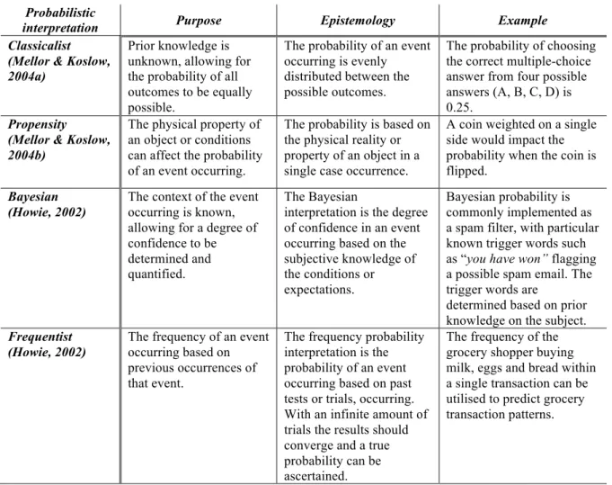
Table 2.3, Shows the four interpretations of probability. Along with the purpose and
epistemology of the four interpretations of probability ... 19
Table 3.1, Shows the reason for research, ontology, epistemology, mode of inquiry for the
four research paradigms. Adapted from Creswell (2014), Mackenzie and Knipe (2006)
and Williamson and Johnson (2013)
... 31
Table 3.2, Shows a confusion matrix used to measure the performance of a classification
learning algorithm.
... 47
Table 3.3, Shows the hardware equipment, specification and a description of the task
conducted on the device used in this study
... 49
Table 3.4, Shows the software, version and a description of the task conducted using the
application within this study
... 50
Table 4.1, Shows the three SSH datasets that will be utilised in this study
... 52
Table 4.2, Shows the number of samples in the input table of the six Kippo SSH honeypots
combined to form SSH dataset one
... 54
Table 4.3, Shows a sample of the transposed and tidied dataset
... 60
Table 4.4, Shows a sample of the formatted, transposed and tidied dataset
... 61
Table 5.1, Shows the precision, accuracy, sensitivity, F1 score and error rate of the classified
instances using the trained Naïve Bayes algorithm for RD1 and FD1. Calculated using
the confusion matrices for each dataset, the measurements are on a scale between 0 and
1, where 1 is the highest.
... 76
Table 5.2, Shows the precision, accuracy, sensitivity, F1 score and error rate of the classified
instances using the trained Naïve Bayes algorithm for RD2 and FD2. Calculated using
the confusion matrices for each dataset, the measurements are on a scale between 0 and
1, where 1 is the highest.
... 79
Table 5.3, Shows the precision, accuracy, sensitivity, F1 score and error rate of the classified
instances using the trained Naïve Bayes algorithm for RD3 and FD3. Calculated using
the confusion matrices for each dataset, the measurements are on a scale between 0 and
1, where 1 is the highest.
... 82
Table 5.4, Shows the mean and standard deviation values for the standard error matrix,
lower endpoint matrix and upper endpoint matrix of the transition matrices generated
by the Markov chain algorithm for RD1 and FD1.
... 86
Table 5.5, Shows the mean and standard deviation values for the standard error matrix,
lower endpoint matrix and upper endpoint matrix of the transition matrices generated
by the Markov chain algorithm for RD2 and FD2.
... 89
Table 5.6, Shows the mean and standard deviation values for the standard error matrix,
lower endpoint matrix and upper endpoint matrix of the transition matrices generated
by the Markov chain algorithm for RD3 and FD3.
... 93
Table 5.7, Shows the results from the initial analysis conducted on the three distinct datasets,
in order to determine the minimum support and confidence values to be set along with
the length of the rules to be extracted.
... 98
VII
Table 5.8, Shows the total number of rules extracted, number of unique rules after removing
the duplicate rules and the percentage of duplicate rules extracted by the Apriori
algorithm applied to RD1 and FD1.
... 98
Table 5.9, Shows the distribution of the support, confidence and lift values for the top 50
support based rules extracted by the Apriori algorithm applied to RD1 and FD1.
... 101
Table 5.10, Shows the total number of rules extracted, number of unique rules after removing
the duplicate rules and the percentage of duplicate rules extracted by the Apriori
algorithm applied to RD2 and FD2.
... 106
Table 5.11, Shows the distribution of the support, confidence and lift values for the top 50
support based rules extracted by the Apriori algorithm applied to RD2 and FD2.
... 109
Table 5.12, Shows the total number of rules extracted, number of unique rules after removing
the duplicate rules and the percentage of duplicate rules extracted by the Apriori
algorithm applied to RD3 and FD3.
... 113
Table 5.13, Shows the distribution of the support, confidence and lift values for the top 50
support based rules extracted by the Apriori algorithm applied to RD3 and FD3.
... 116
Table 5.14, Shows the total number of rules extracted, number of unique rules after removing
the duplicate rules and the percentage of duplicate rules extracted by the Eclat
algorithm applied to RD and FD1.
... 121
Table 5.15, Shows the distribution of the support, confidence and lift values for the top 50
support based rules extracted by the Eclat algorithm applied to RD1 and FD1.
... 125
Table 5.16, Shows the total number of rules extracted, the number of unique rules after
removing the duplicate rules and the percentage of duplicate rules extracted by the
Eclat algorithm applied to RD2 and FD2.
... 129
Table 5.17, Shows the distribution of the support, confidence and lift values for the top 50
support based rules extracted by the Eclat algorithm applied to RD2 and FD2.
... 132
Table 5.0.18, Shows the total number of rules extracted, number of unique rules after
removing the duplicate rules and the percentage of duplicate rules extracted by the
Eclat algorithm applied to RD3 and FD3.
... 136
Table 5.19, Shows the distribution of the support, confidence and lift values for the top 50
support based rules extracted by the Eclat algorithm applied to RD3 and FD3.
... 140
Table 5.20, Shows the aggregated True Positive (TP) rate of the trained Naïve Bayes
classifier applied to the test sets of the three reduced datasets and their respective full
datasets, along with the difference between the rates.
... 144
Table 5.21, Shows the aggregated degree of freedom for reduced datasets and their
respective full datasets calculated by the Markov chain algorithm.
... 145
Table 5.22, Shows the aggregated unique rule sets for the reduced datasets and their
respective full datasets after the duplicated rules had been removed by the Apriori
algorithm
... 145
Table 5.23, Shows the aggregated unique rule sets for the reduced datasets and their
respective full datasets after the duplicated rules had been removed by the Eclat
algorithm
... 146
Table 5.24, Shows the aggregated precision of the trained Naïve Bayes classifier applied to
the three reduced datasets and their respective full datasets
... 147
Table 5.25, Shows the mean and standard deviation values for the standard error matrix,
lower endpoint matrix and upper endpoint matrix of the transition matrices generated
by the Markov chain algorithm for the three reduced datasets and their respective full
datasets.
... 149
Table 5.26, Shows the distribution of the support, confidence and lift values for the top 50
support based rules extracted by the Apriori algorithm applied to the three reduced
datasets and the respective full datasets.
... 150
VIII
Table 5.27, Shows the distribution of the support, confidence and lift values for the top 50
support based rules extracted by the Eclat algorithm applied to the three reduced
datasets and the respective full datasets.
... 151
Table 5.28, Shows the mean processing time in seconds(s) for the Naïve Bayes, Markov
chain, Apriori and Eclat algorithms to process reduced datasets and their respective full
datasets iterated 100 times (Test 1) and 1,000 times (Test 2)
... 153
IX
Table of Figures
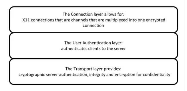
Figure 2.1, illustrates the three main components of SSH-2, transport layer protocol, user
authentication layer protocol and connection layer protocol ... 12
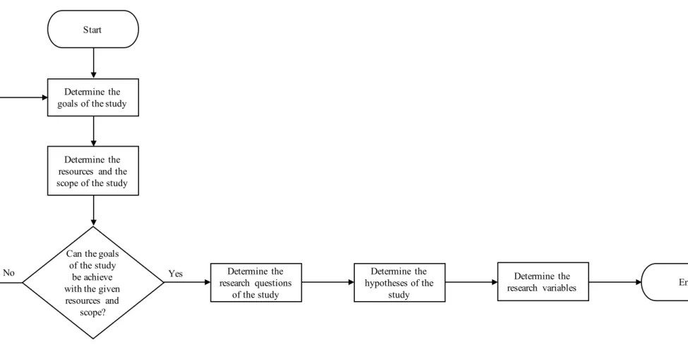
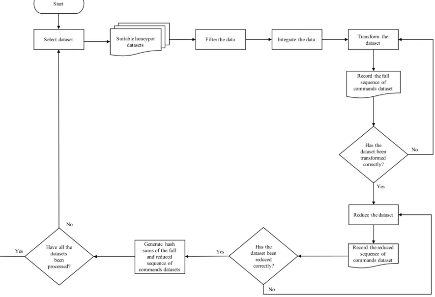
Figure 3.0.1, Illustrates the research procedure designed for this study consisting of five
phases. ... 37
Figure 3.0.2, Illustrates a flowchart showing the process of phase 1, the project
understanding phase ... 38
Figure 3.0.3, Illustrates a flowchart showing the process of phase 2, the data understanding
phase. ... 40
Figure 3.0.4, Illustrates a flowchart showing the process of phase 3, the pre-processing
understanding phase. ... 42
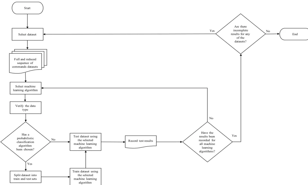
Figure 3.0.5, Illustrates a flowchart showing the process of phase 4, the experimental phase.
... 44
Figure 3.0.6, Illustrates a flowchart showing the process of phase 5, evaluation and analysis
phase ... 46
Figure 4.0.1, Illustrates the MySQL dataset structure for Kippo honeypot (Rabadia et al.,
2017) ... 53
Figure 4.0.2, Depicts the five steps in the pre-processing procedure used in this study. The
data wrangling step is outside the boundary as the step will occur prior to applying a
chosen machine learning algorithm. ... 57
Figure 4.0.3, Depicts the three stages of data massaging in the data filtering step of the
pre-processing procedure ... 64
Figure 5.0.1, Illustrates the processing time in seconds(s) for the Naïve Bayes algorithm to
process RD1 and FD1. The process was iterated 100 times, with the black lines
represent the mean processing time for the datasets after the outliers had been removed.
... 77
Figure 5.0.2, Illustrates the processing time in seconds(s) for the Naïve Bayes algorithm to
process RD1 and FD1. The process was iterated 1,000 times, with the black lines
represent the mean processing time for the datasets after the outliers had been removed.
... 77
Figure 5.0.3, Illustrates the processing time in seconds(s) for the Naïve Bayes algorithm to
process RD2 and FD2. The process was iterated 100 times, with the black lines
represent the mean processing time for the datasets after the outliers had been removed.
... 80
Figure 5.0.4, Illustrates the processing time in seconds(s) for the Naïve Bayes algorithm to
process RD2 and FD2. The process was iterated 1,000 times, with the black lines
represent the mean processing time for the datasets after the outliers had been removed.
... 80
Figure 5.0.5, Illustrates the processing time in seconds(s) for the Naïve Bayes algorithm to
process RD3 and FD3. The process was iterated 100 times, with the black lines
represent the mean processing time for the datasets after the outliers had been removed.
... 83
Figure 5.0.6, Illustrates the processing time in seconds(s) for the Naïve Bayes algorithm to
process RD3 and FD3. The process was iterated 1,000 times, with the black lines
represent the mean processing time for the datasets after the outliers had been removed.
... 83
Figure 5.0.7, Illustrates the processing time in seconds(s) for the Markov chain algorithm to
X
iterated 100 times, with the black lines represent the mean processing time for the
datasets after the outliers had been removed. ... 87
Figure 5.0.8, Illustrates the processing time in seconds(s) for the Markov chain algorithm to
converge the transition matrices for RD1 and FD1, scaled to log
10. The process was
iterated 1,000 times, with the black lines represent the mean processing time for the
datasets after the outliers had been removed. ... 88
Figure 5.0.9, Illustrates the processing time in seconds(s) for the Markov chain algorithm to
converge the transition matrices for RD2 and FD2. The process was iterated 100 times,
with the black lines represent the mean processing time for the datasets after the outliers
had been removed. ... 91
Figure 5.0.10, Illustrates the processing time in seconds(s) for the Markov chain algorithm to
converge the transition matrices for the RD2 and FD2. The process was iterated 1,000
times, with the black lines represent the mean processing time for the datasets after the
outliers had been removed. ... 91
Figure 5.0.11, Illustrates the processing time in seconds(s) for the Markov chain algorithm to
converge the transition matrices for RD3 and FD3. The process was iterated 100 times,
with the black lines represent the mean processing time for the datasets after the outliers
had been removed. ... 94
Figure 5.0.12, Illustrates the processing time in seconds(s) for the Markov chain algorithm to
converge the transition matrices for RD3 and FD3. The process was iterated 1,000
times, with the black lines represent the mean processing time for the datasets after the
outliers had been removed. ... 95
Figure 5.0.13, Illustrates a scatter plot of support, confidence and lift values of the total rule
set extracted by the Apriori algorithm from FD1. ... 99
Figure 5.0.14, Illustrates a scatter plot of support, confidence and lift values of the total rule
set extracted by the Apriori algorithm from RD1. ... 99
Figure 5.0.15, Illustrates a scatter plot of support, confidence and lift values of the top 50
support based rule set extracted by the Apriori algorithm from FD1. ... 100
Figure 5.0.16, Illustrates a scatter plot of the support, confidence and lift values of the top 50
support based rule set extracted by the Apriori algorithm from RD1. ... 101
Figure 5.0.17, is a visual representation of the support, confidence and lift values of the top
50 support based rule set extracted by the Apriori algorithm from FD1. ... 102
Figure 5.0.18, is a visual representation of the support, confidence and lift values of the top
50 support based rule set extracted by the Apriori algorithm from RD1. ... 103
Figure 5.0.19, Illustrates the processing time in seconds(s) of the Apriori algorithm process
RD1 and FD1. The process was iterated 100 times, with the black lines represent the
mean processing time for the datasets after the outliers had been removed. ... 104
Figure 5.0.20, Illustrates the processing time in seconds(s) of the Apriori algorithm process
RD1 and FD1. The process was iterated 1,000 times, with the black lines represent the
mean processing time for the datasets after the outliers had been removed. ... 105
Figure 5.0.21, Illustrates a scatter plot of support, confidence and lift values of the total rule
set extracted by the Apriori algorithm from FD2. ... 106
Figure 5.0.22, Illustrates a scatter plot of support, confidence and lift values of the total rule
set extracted by the Apriori algorithm from RD2. ... 107
Figure 5.0.23, Illustrates a scatter plot of support, confidence and lift values of the top 50
support based rule set extracted by the Apriori algorithm from FD2. ... 108
Figure 5.0.24, Illustrates a scatter plot of the support, confidence and lift values of the top 50
support based rule set extracted by the Apriori algorithm from RD2. ... 108
Figure 5.0.25, is a visual representation of the support, confidence and lift values of the top
XI
Figure 5.0.26, is a visual representation of the support, confidence and lift values of the top
50 support based rule set extracted by the Apriori algorithm from RD2. ... 110
Figure 5.0.27, Illustrates the processing time in seconds(s) of the Apriori algorithm process
RD2 and FD2. The process was iterated 100 times, with the black lines represent the
mean processing time for the datasets after the outliers had been removed. ... 111
Figure 5.0.28, Illustrates the processing time in seconds(s) of the Apriori algorithm process
the RD2 and FD2. The process was iterated 1,000 times, with the black lines represent
the mean processing time for the datasets after the outliers had been removed. ... 112
Figure 5.0.29, Illustrates a scatter plot of support, confidence and lift values of the total rule
set extracted by the Apriori algorithm from FD3. ... 113
Figure 5.0.30, Illustrates a scatter plot of support, confidence and lift values of the total rule
set extracted by the Apriori algorithm from RD3. ... 114
Figure 5.0.31, Illustrates a scatter plot of support, confidence and lift values of the top 50
support based rule set extracted by the Apriori algorithm from FD3. ... 115
Figure 5.0.32, Illustrates a scatter plot of the support, confidence and lift values of the top 50
support based rule set extracted by the Apriori algorithm from RD3. ... 115
Figure 5.0.33, is a visual representation of the support, confidence and lift values of the top
50 support based rule set extracted by the Apriori algorithm from FD3. ... 117
Figure 5.0.34, is a visual representation of the support, confidence and lift values of the top
50 support based rule set extracted by the Apriori algorithm from RD3. ... 117
Figure 5.0.35, Illustrates the processing time in seconds(s) of the Apriori algorithm process
RD3 and FD3. The process was iterated 100 times, with the black lines represent the
mean processing time for the datasets after the outliers had been removed. ... 119
Figure 5.0.36, Illustrates the processing time in seconds(s) of the Apriori algorithm process
RD3 and FD3. The process was iterated 1,000 times, with the black lines represent the
mean processing time for the datasets after the outliers had been removed. ... 119
Figure 5.0.37, Illustrates a scatter plot of support, confidence and lift values of the total rule
set extracted by the Eclat algorithm from FD1. ... 122
Figure 5.0.38, Illustrates a scatter plot of support, confidence and lift values of the total rule
set extracted by the Eclat algorithm from RD1. ... 122
Figure 5.0.39, Illustrates a scatter plot of support, confidence and lift values of the top 50
support based rule set extracted by the Eclat algorithm from FD1. ... 123
Figure 5.0.40, Illustrates a scatter plot of the support, confidence and lift values of the top 50
support based rule set extracted by the Eclat algorithm from RD1. ... 124
Figure 5.0.41, is a visual representation of the support, confidence and lift values of the top
50 support based rule set extracted by the Eclat algorithm from FD1. ... 125
Figure 5.0.42, is a visual representation of the support, confidence and lift values of the top
50 support based rule set extracted by the Eclat algorithm from RD1. ... 126
Figure 5.0.43, Illustrates the processing time in seconds(s) of the Eclat algorithm process
RD1 and FD1. The process was iterated 100 times, with the black lines represent the
mean processing time for the datasets after the outliers had been removed. ... 127
Figure 5.0.44, Illustrates the processing time in seconds(s) of the Eclat algorithm process
RD1 and FD1. The process was iterated 1,000 times, with the black lines represent the
mean processing time for the datasets after the outliers had been removed. ... 128
Figure 5.0.45, Illustrates a scatter plot of support, confidence and lift values of the total rule
set extracted by the Eclat algorithm from FD2. ... 129
Figure 5.0.46, Illustrates a scatter plot of support, confidence and lift values of the total rule
set extracted by the Eclat algorithm from RD2. ... 130
Figure 5.0.47, Illustrates a scatter plot of support, confidence and lift values of the top 50
XII
Figure 5.0.48, Illustrates a scatter plot of the support, confidence and lift values of the top 50
support based rule set extracted by the Eclat algorithm from RD2. ... 131
Figure 5.0.49, is a visual representation of the support, confidence and lift values of the top
50 support based rule set extracted by the Eclat algorithm from FD2. ... 133
Figure 5.0.50, is a visual representation of the support, confidence and lift values of the top
50 support based rule set extracted by the Eclat algorithm from RD2. ... 133
Figure 5.0.51, Illustrates the processing time in seconds(s) of the Eclat algorithm process
RD2 and FD2. The process was iterated 100 times, with the black lines represent the
mean processing time for the datasets after the outliers had been removed. ... 134
Figure 5.0.52, Illustrates the processing time in seconds(s) of the Eclat algorithm process
RD2 and FD2. The process was iterated 1,000 times, with the black lines represent the
mean processing time for the datasets after the outliers had been removed. ... 135
Figure 5.0.53, Illustrates a scatter plot of support, confidence and lift values of the total rule
set extracted by the Eclat algorithm from FD3. ... 137
Figure 5.0.54, Illustrates a scatter plot of support, confidence and lift values of the total rule
set extracted by the Eclat algorithm from RD3. ... 138
Figure 5.0.55, Illustrates a scatter plot of support, confidence and lift values of the top 50
support based rule set extracted by the Eclat algorithm from FD3. ... 138
Figure 5.0.56, Illustrates a scatter plot of the support, confidence and lift values of the top 50
support based rule set extracted by the Eclat algorithm from RD3. ... 139
Figure 5.0.57, is a visual representation of the support, confidence and lift values of the top
50 support based rule set extracted by the Eclat algorithm from FD3. ... 141
Figure 5.0.58, is a visual representation of the support, confidence and lift values of the top
50 support based rule set extracted by the Eclat algorithm from RD3. ... 141
Figure 5.0.59, Illustrates the processing time in seconds(s) of the Eclat algorithm process
RD3 and FD3. The process was iterated 100 times, with the black lines represent the
mean processing time for the datasets after the outliers had been removed. ... 142
Figure 5.0.60, Illustrates the processing time in seconds(s) of the Eclat algorithm process
RD3 and FD3. The process was iterated 1,000 times, with the black lines represent the
mean processing time for the datasets after the outliers had been removed. ... 143
1
1 Introduction
1.1 Background of the Study
Mitigating the exposure of digital assets is becoming increasingly imperative. Estimates have shown cybercrime costs Australia one billion AUD each year (The Department of the Prime Minister and Cabinet, 2016). A defence in depth cyber security strategy can mitigate the exposure of these digital assets. Intrusion detection approaches are deployed by Intrusion Detection Systems (IDSs), to monitor network traffic and trigger an alert, or an appropriate response when unauthorised activities are detected on a network. The concept of intrusion detection was first introduced in 1980 by Anderson (1980). Traditionally there are two types of intrusion detection approaches that are implemented, signature or misuse based, and anomaly based.
The signature or misuse based detection category involves comparing the signatures of current network traffic to a database of known bad signatures of network traffic. If a reasonable match is found an alert is triggered for possible adversarial activities on the network (Sultana, Chilamkurti, Peng, & Alhadad, 2018). The signature or misuse based detection approaches are known for precisely classifying known bad network traffic. However, unknown or new activities go undetected, as the signatures have not yet been generated for a comparison to take place. Previously unknown or new vulnerabilities exposed by adversarial activities (Bilge & Dumitra, 2012) are colloquially known as zero day attacks.
Anomaly based detection approaches involve generating a baseline of normal network traffic behaviour. The generated baseline is then compared to the current network traffic observed. Any nonconformities to the baseline are considered to be anomalous traffic, and an alert is triggered for possible adversarial activities detected on the network (Sultana et al., 2018). Though, any authorised network traffic that does not conform to the baseline also triggers an alert. This impacts the precision of anomaly based intrusion detection approaches to classify network traffic. Unlike the signature or misuse based detection category, these approaches can identify zero day attacks as anomalous traffic generally results in nonconforming traffic to the baseline.
Precision and efficiency are key performance attributes of an intrusion detection approach. A detection approach needs to be precise at detecting both, known and unknown adversarial activities on a network. Along with precisely detecting adversarial activities on a network, an intrusion detection approach needs to efficiently process the network traffic. Allowing for a timely detection of an adversary on the network prior to protected assets being attacked and subsequently compromised (Masduki & Ramli, 2016).
2
The efficiency of an intrusion detection approach is significant, as predictions show on a global scale the number of Exabytes (1018) per month of IP traffic sent is set to increase with the passing of each year. Table 1.1 shows there is an annual growth rate of 24% in the Exabytes per month of IP traffic between the years of 2016 until 2021 (Cisco, 2017). Table 1.1 is adapted from Cisco’s 2017 white paper, that forecasted the trends and predictions of global internet traffic (Cisco, 2017). The increase in Internet traffic can also be aligned with the increase in other network traffic such as that exhibited on organisational networks. Processing the increase in network traffic and precisely detecting adversarial activities is a major challenge.
Table 1.1, Shows the global forecasted increase in the Exabytes per month of Internet Protocol (IP) traffic sent for the years between 2016 and 2021. Adapted from (Cisco, 2017)
Year Exabytes (1018) per Month
2016 96 2017 122 2018 151 2019 186 2020 228 2021 278
Typically, intrusion detection approaches monitor and analyse network flow data or packet level data. Network flow data consists of monitoring and analysing features associated with the flow of data through the network. These features include the source and destination IP address, along with the source and destination port numbers (Hellemons et al., 2012). Monitoring and analysing packet level data have more processing and storage overheads compared to analysing network flow data because there are more features that can be extracted from packet level data compared to network flow data. Examples of additional features that can be extracted include, protocol type and the number of root connections to name a few. This impacts the processing and storage overheads of packet level data analysis.
Deep Packet Inspection (DPI) is the further examination of packet level data to gain a further insight into network traffic communications and can be used for real-time analysis and off-line analysis. There are many uses of DPI within the cyber security domain, including for intrusion detection purposes. The additional knowledge gained from a DPI can be used for cyber defence optimisation, malicious software detection and user activity monitoring including adversary activity identification (Rabadia, Valli, Ibrahim, & Baig, 2017).
The publicly available (open-source) datasets are commonly utilised for benchmarking and evaluating intrusion detection approaches. Since the features required for a DPI are omitted within the open-source datasets, data acquired from three distinct Secure Shell (SSH) honeypots have been utilised for this study. SSH is used for point to point communication over an insecure network, creating an encrypted
3
tunnel for remote communications and access (Tatu Ylonen, 2017c). SSH was developed in 1995 by Tatu Ylonen and was a response to a password sniffing attack against Helsinki University of Technology. This first version is referred to as SSH-1. The SSH service is predominately targeted by adversaries to attempt to gain unauthorised remote access to a system.
This study aims to investigate adversarial SSH commands for a pattern-based intrusion detection approach. Seeing as SSH is one of the most predominant methods of remotely accessing a systems compared to Telnet and is also a prime vector for cyber criminal activities. Pattern-based intrusion detection approaches discover and extract patterns within network traffic data for adversarial activity detection. Some of the most common means of implementing pattern-based intrusion detection approaches are utilising machine learning algorithms to analyse network traffic. Machine learning is the application of learning algorithms to extract knowledge from data to determine patterns between data points and make predictions. This study utilises selected machine learning algorithms to extract patterns from adversarial SSH commands. The selected machine learning algorithms are the Naïve Bayes, Markov chain, Apriori and Equivalence Class Transformation (Eclat) algorithms.
There are two main approaches for enhancing the precision and efficiency of pattern-based intrusion detection approaches for the SSH service. These involve implementing the use of hybrid algorithms and feature selection of the dataset. Hybrid algorithms are developed by combining two or more algorithms. The notion of a hybrid algorithm is combining machine learning algorithms that complement each other. Algorithms belonging to different machine learning categories are typically combined, such as clustering and classification algorithms (Soheily-Khah, Marteau, & Béchet, 2018). While feature selection is choosing relevant attributes within a dataset that will allow for additional information to be extracted by classifying the dataset based on the selected features. The pre-processing phase is a critical process when applying machine learning algorithms (Malley, Ramazzotti, & Wu, 2016). In the pre-processing phase, the datasets are processed and prepared to be applied to the selected machine learning algorithms. The feature selection process takes place in the pre-processing phase. The pre-processing phase also includes a data reduction step to enhance the performance of the selected machine learning algorithms. Data reduction involves generating a reduced dataset that evenly and coherently represents the respective full dataset. For this study precision is in reference to correctly identifying patterns in sequential adversarial commands within the given datasets. Furthermore for this study efficiency is in reference to the processing time for the selected machine learning algorithms to extract the patterns from the given datasets.
4
1.2 Purpose and Scope of Study
The pattern-based intrusion detection approach investigated in this study focuses on adversary command data, as a means of detecting adversaries on the monitored network. In conjunction with efficiently processing the network data to timely detect adversaries. This study aims to contribute to the knowledge domain of pattern-based intrusion detection approaches for the SSH service.
The focus of this study was the use of adversary command patterns for intrusion detection purposes, DPI was required to ascertain the adversary command data. The examination of existing literature has shown there has been research conducted in the domain of adversary based intrusion detection approaches utilising DPI (Pimenta Rodrigues et al., 2017). Although there are gaps in the knowledge domain of DPI, this thesis aims to contribute in terms of pattern identification within a sequence of adversary interaction commands. Together with evaluating whether a reduced sequence of command dataset can be efficiently processed and whether the patterns extracted are more precise compared to the respective full dataset.
A pre-processing procedure that encompasses feature selection and data reduction is deployed for this study and is to be applied to the acquired datasets prior to the application of the chosen machine learning algorithms. The selected machine learning algorithms have been utilised to extract patterns from a sequence of adversarial SSH interaction commands. The selected machine learning algorithms are the Naïve Bayes, Markov chain, Apriori and Equivalence Class Transformation (Eclat) algorithms. The Naïve Bayes and Markov chain algorithms are probabilistic classification algorithms and have been selected as they aligned with the machine learning problem of classification and the Bayesian theorem interpretation of probability. The Apriori and Eclat algorithms are association rule mining algorithms and have been selected as they aligned with the machine learning problem of association and the frequentist theorem interpretation of probability.
5
1.3 Research Questions and associated Hypotheses
The research questions and the associated hypotheses of this thesis are presented below.
RQ1: Is there an increase in the number of patterns extracted from the reduced datasets by the machine learning algorithms, compared to the number of patterns extracted from their respective full datasets?
H1: More class patterns can be extracted from the reduced sequence of commands datasets, compared to those extracted from their respective full datasets by the selected probabilistic classification algorithms.
H2: More patterns can be extracted from the rule sets of the reduced sequence of commands datasets, compared to those extracted from their respective full datasets by the selected association rule mining algorithms.
RQ2: Are the extracted patterns from the reduced datasets by the machine learning algorithms overall more precise, compared to those extracted from their relevant full datasets?
H3: The class patterns extracted by the probabilistic classification algorithms from the reduced sequence of commands datasets are more precise, compared to those extracted from their respective full datasets.
H4: The patterns extracted from the rule sets by the association rule mining algorithms from the reduced sequence of commands datasets are more precise, compared to those rule sets extracted from their respective full datasets.
RQ3: Are the machine learning algorithms more efficient at extracting patterns from
the reduced datasets, compared to the processing time of their respective full datasets?
H5: The probabilistic classification algorithms are more efficient at extracting patterns from the reduced sequence of commands datasets, compared to their respective full datasets.
H6: The association rule mining algorithms are more efficient at extracting patterns from the rule set for the reduced sequence of commands datasets, compared to their respective full datasets.
6
1.4 Thesis Structure
The structure of the remaining thesis is as follows.
Chapter Two is the Literature Review. This is the exploration of the existing literature surrounding this study in order to identify the gap in the knowledge this study intends to fill. Literature surrounding DPI, for adversarial pattern-based intrusion detection approaches are explored, along with identifying the suitable machine learning algorithms to be utilised for this study.
Chapter Three is the Research Methodology and Design for this study. The research approach that underpins this study is established. The research procedure, encompassing five phases is outlined. Further, an overview of data analysis is presented along with the equipment, and resources utilised for this study.
Chapter Four is the Preliminary analysis for this study. Initial exploration and analysis of the acquired datasets are conducted in this chapter along with applying the pre-processing procedure developed for this study. On the conclusion of this chapter, the three SSH honeypot datasets are processed resulting in three reduced datasets and their respective full datasets.
Chapter Five is the Results Chapter. In this chapter, the results collected from the experiments conducted to test the hypotheses of this study. The experiments encompass applying the selected machine learning algorithms to the reduced datasets and their respective full datasets.
Chapter Six is the Discussion and Findings Chapter. The results obtained from the experiments conducted to test the hypotheses in relation to addressing the research questions are analysed. As well as presenting the implications of this study along with a critical review of this study.
Chapter Seven is the Conclusion. In this chapter, an overview of this study and the contributions this thesis has made to the knowledge domain are outlined. Finally, the recommendations and potential further research areas are outlined.
7
2 Literature Review
2.1 Overview of Intrusion Detection Approaches
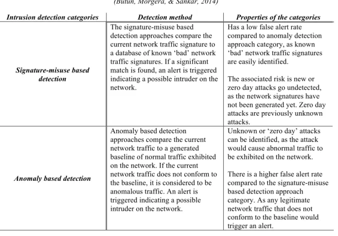
This study investigated whether patterns extracted from sequential adversarial SSH commands can be utilised as a pattern-based intrusion detection approach. A pattern-based intrusion detection approach discovers and extracts patterns from network traffic to detect adversaries on the network. The signature-misuse based and anomaly based detection are the two common intrusion detection categories. The detection methods and properties of these common intrusion detection categories are presented in Table 2.1.
Table 2.1, Shows the detection methods and properties of the two common intrusion detection categories (Butun, Morgera, & Sankar, 2014)
Intrusion detection categories Detection method Properties of the categories
Signature-misuse based detection
The signature-misuse based detection approaches compare the current network traffic signature to a database of known ‘bad’ network traffic signatures. If a significant match is found, an alert is triggered indicating a possible intruder on the network.
Has a low false alert rate compared to anomaly detection approach category, as known ‘bad’ network traffic signatures are easily identified.
The associated risk is new or zero day attacks go undetected, as the network signatures have not been generated yet. Zero day attacks are previously unknown attacks.
Anomaly based detection
Anomaly based detection approaches compare the current network traffic to a generated baseline of normal traffic exhibited on the network. If the current network traffic does not conform to the baseline, it is considered to be anomalous traffic. An alert is triggered indicating a possible intruder on the network.
Unknown or ‘zero day’ attacks can be identified, as the attack would cause abnormal traffic to be exhibited on the network. There is a higher false alert rate compared to the signature-misuse based detection approach
category. As any legitimate network traffic that does not conform to the baseline would trigger an alert.
Precision and efficiency are key attributes of an intrusion detection approach. An intrusion detection approach needs to precisely detect adversaries on the network. There should be a low rate of misclassified network traffic (false alert rate) and high rate of correctly classified network traffic (true alert rate. An intrusion detection approach also needs to be efficient at detecting adversaries on a network to prevent the exposure of assets in a timely manner (Masduki & Ramli, 2016). For this study precision is in reference to correctly identifying patterns in sequential adversarial commands within the given datasets. Furthermore for this study efficiency is in reference to the processing time for the selected machine learning algorithms to extract the patterns from the given datasets.
8
An intrusion detection approach either monitors packet level data or network flow data. Network flow data consists of monitoring source IP, destination IP, source port and destination port along with the number of packets sent per flow (Hellemons et al., 2012). Whereas, packet level monitoring also monitors the protocol type and the number of root connections to name a few attributes. Consequently, monitoring network flow data has less processing and storage overheads compared to monitoring packet level data. However, additional information can be extracted from packet level data compare to network flow data. Within the literature open-source or publicly available datasets are typically utilised when conducting studies on enhancing intrusion detection approaches.
2.1.1 Open-source Intrusion Detection Datasets
The Defence Advanced Research Projects Agency (DARPA) released an intrusion detection dataset in 1998, known as the DARPA 1998 dataset. The DARPA 1998 dataset was derived from a simulated Air Force base network that encompasses fictitious Internet traffic, malicious scripts, injection attacks and Sun BSM attack data (DARPA, 1998). In the year 1999, the DARPA 1998 intrusion detection dataset was revised to contain supplementary attacks as well as Windows NT attack data and is referred to as the DARPA 99 dataset (DARPA, 1999). However, that same year the Knowledge Discovery in Databases (SIGKDD) Cup 99 dataset was released. The data in the KDD cup 99 dataset is formulated from the DARPA 1999 dataset (SIGKDD, 1999). The KDD Cup 99 dataset was originally used for The Third International KDD and Data Mining Tools Competition. Since then the KDD Cup 99 dataset has become a benchmark dataset in the domain of intrusion detection research (Gharib, Sharafaldin, Lashkari, & Ghorbani, 2016; Tavallaee, Bagheri, Lu, & Ghorbani, 2009).
The KDD Cup 99 dataset became the benchmark dataset, as unlike the DARPA 99 dataset users were not required to convert the data from a raw format to a readable format, as well as the necessary features had already been extracted. The KDD Cup 99 dataset contains 14 additional attacks compared to the DARPA 99 dataset. These additional 14 attacks are only seen in the test dataset. Allowing for a detection approach to be evaluated based on unseen attacks, similar to ‘zero day’ attacks that are seen in real network traffic (SIGKDD, 1999; Tavallaee et al., 2009). Consequently, there are inherent issues with redundant data within the KDD Cup 99 dataset since it is derived from the DARPA 99 dataset, resulting in classification bias. 78.05% of the KDD Cup 99 training dataset is redundant data and 75.15% of the test dataset is redundant (Tavallaee et al., 2009).
In 2009, Tavallaee et al. (2009) presented a revised version of the KDD Cup 99 dataset, known as the NSL-KDD dataset. The NSL-KDD dataset addresses some of the issues associated with the KDD Cup 99 dataset. Redundant records had been removed to avoid classification bias. Additionally, allowing data to be randomly selected from the training and testing sets. The data chosen to be included in the
9
NSL-KDD dataset, have been chosen based on different levels of difficulties to reflect the original KDD Cup 99 dataset for different machine learning algorithms to be tested. Both the KDD Cup 99 dataset and the NSL-KDD dataset have four categories of attacks, Denial of Service (Koch, Golling, & Rodosek), Probe, Remote to Local (R2L) and User to Root (U2R). Additionally, both datasets have 41 features with varying data types between nominal, continuous and binary data types. However, none of the 41 features within the KDD Cup 99 dataset nor the NSL-KDD dataset contain adversary command data. The datasets have issues with high levels of redundant data as well as the absence of adversary command data. From exploring the DARPA 98, DARPA 99, KDD Cup 99 and NSL-KDD datasets are not suitable to be utilised for this study. It has been ~20 years since the benchmark KDD Cup 99 dataset was released and ~10 years since the improved NSL-KDD dataset was released. The focus of this study was to extract patterns from adversarial command interaction data, in reference to the commands utilised by adversaries while interacting with a system.
Other intrusion detection datasets include the PREDICT dataset, UNSW-NB15 dataset and KYOTO honeypot dataset (Gharib et al., 2016). The PREDICT dataset was developed by the Department of Homeland Security (DHS) and the Centre of Applied Internet Data Analysis (CAIDA) released to the public in 2016. Access to the dataset is restricted to researchers based in the United States and approved DHS countries. Although Australia is among the list of approved countries, the dataset was not suitable for this study due to risks of data exposure and publication restrictions (CAIDA, 2016; Impact Cyber Trust, 2017). The UNSW-NB15 dataset was released to the public in 2015, it was developed by academics at the University of New South Wales the dataset consists of 49 features and nine attack types (Moustaf & Slay, 2016; Moustafa & Slay, 2015) . Adversary command data is absent deeming the dataset unsuitable for this study. The Kyoto honeypot dataset, was generated by the Kyoto University between 2009 and 2015. The data is collected from Nepenthes low interaction honeypots. The Kyoto dataset contains a total of 24 features (Jungsuk Song, Hiroki Takakura, & Okabe; Kyoto University, 2015). Similar to the previous intrusion detection datasets, the Kyoto honeypot dataset does not contain adversary command data thus deeming the dataset unsuitable for this study.
From evaluating the possible open-source datasets, none of the datasets explored contains adversarial command data. The adversarial command data required for this study was gathered by honeypots. Honeypots are Intrusion Detection Systems (IDSs) (SURF cert IDS, 2013) tools used to gather data on adversary activities.
2.1.2 Honeypots
Honeypots are decoy systems intended to be attacked with the purpose of gathering data of adversarial interactions with the system. These systems are predominantly located in the Demilitarised Zone
10
(DMZ) of a network, to separate the decoy system from the real network (The Honeynet Project, 2011). There are two categories of honeypots that can be deployed depending on the purpose: production honeypots and research honeypots. Production honeypots are commonly utilised by organisations to gather data on adversaries attempting to gain access to their infrastructure. The data collected from the production honeypots can be used by an organisation to determine potential vulnerabilities in their cyber security strategy that could be exploited by adversaries. This allows the organisation to address the vulnerabilities reducing the probability of adversaries gaining unauthorised access to the network. While data collected from the research honeypots are used to analyse the techniques and methods adversaries use to gain unauthorised access. Data collected from research honeypots can be used to assist organisations in improving their intrusion detection policies and rules. There are three types of honeypots that can be implemented depending on the requirements of the deployment.
The types of honeypots are based on the level of interaction that occurs between the system and the adversary. In Table 2.2, the properties of the different types honeypots and examples of existing Secure Shell (SSH) honeypots are presented. The three types of honeypots are, high interaction, medium interaction and low interaction, honeypots.
Table 2.2, Shows the three types of honeypots and their properties including examples of existing SSH honeypots (Rabadia et al., 2017)
Honeypot type Properties Example
High interaction
These honeypots emulate a fully
functioning system. Adversaries are led to believe they are interacting with a real system. The high interaction honeypots have a similar configuration process to a real system, consequentially the
maintenance requirements are demanding.
• HonSSH
Medium interaction
These honeypots exhibit selected
functionalities of a real system, for example, a SSH session. As a result, the configuration process is simpler than a high-interaction honeypot but the maintenance required is more demanding than a low-interaction honeypot.
• Kippo SSH
• Cowrie SSH
Low interaction
These hosts have minimal functionalities compared to a real system. They are simple to configure with low maintenance
requirements. Adversaries have minimal interactions with the host compared with a high interaction honeypot.
• Honeyd
The SSH protocol is the selected network traffic chosen to be investigated. Seeing as SSH is one of the most predominant methods of remotely accessing a systems compared to Telnet and is also a prime vector for cyber criminal activities. Since the focus of this study is on a selected network traffic, a medium interaction honeypot was appropriate for this study. A medium interaction honeypot has more
11
functionalities that are similar to a real system compared to a low interaction honeypot. There are also fewer maintenance requirements compared to a high interaction honeypot. Research based honeypots had been chosen as the data gathered was for academic in this study.
The data acquired for this study had been collected from the Kippo and Cowrie medium interaction SSH honeypots. Kippo SSH honeypots had been adapted from Kojoney honeypots, a low interaction SSH honeypot. The Kippo SSH honeypot was released in 2009 and actively developed until October 2016 (Desaster, 2016). Cowrie developer Michel Oosterhof was a former contributor to the Kippo SSH honeypot project. But after no longer actively being developed he launched and continues to develop the Cowrie SSH honeypot.
In both honeypots, a fake file system can be added and removed, adversaries can interact with a fake file system, reply to attacks and the files downloaded by an adversary are saved for later inspection. The Kippo and Cowrie SSH honeypots are both written in Python2.7 and use the Twisted library to emulate a SSH session (Michel Oosterhof, 2018a). The honeypots log forced attempts to gain unauthorised access to the systems as well as the shell session interactions between the honeypot and the adversary.
2.1.2.1 Secure Shell (SSH) Protocol
SSH is used for point to point communications over an insecure network essentially creating an encrypted tunnel for remote communication (Tatu Ylonen, 2017c). SSH was developed in 1995 by Tatu Ylonen and was a response to a password sniffing attack against Helsinki University of Technology and is referred to as SSH-1. The SSH protocol was initially introduced to replace the Telnet protocol due to the lack of encryption. SSH File Transfer Protocol (SFTP) (Tatu Ylonen, 2017b) runs over the SSH protocol and was introduced to replace the insecure File Transfer Protocol (FTP) (Tatu Ylonen, 2017a).
By default, SSH runs on the Transmission Control Protocol (TCP) and User Datagram Protocol (UDP) on port 22. The protocol was taken to a working group at the Internet Engineering Task Force (IETF) for standardisation and evolved into SSH-2. In 2006, SSH-2 was assigned a Request For Comment (Network Working Group, 2006b) number and is currently the widely used version of SSH. Figure 2.1, illustrates the three main components of SSH-2, transport layer protocol, user authentication layer protocol and connection layer protocol.