University of Tennessee, Knoxville
Trace: Tennessee Research and Creative
Exchange
Doctoral Dissertations Graduate School
12-2007
Parametric and Non-Parametric Regression Tree
Models of the Strength Properties of Engineered
Wood Panels Using Real-time Industrial Data
Timothy Mark YoungUniversity of Tennessee - Knoxville
This Dissertation is brought to you for free and open access by the Graduate School at Trace: Tennessee Research and Creative Exchange. It has been accepted for inclusion in Doctoral Dissertations by an authorized administrator of Trace: Tennessee Research and Creative Exchange. For more
Recommended Citation
Young, Timothy Mark, "Parametric and Non-Parametric Regression Tree Models of the Strength Properties of Engineered Wood Panels Using Real-time Industrial Data. " PhD diss., University of Tennessee, 2007.
To the Graduate Council:
I am submitting herewith a dissertation written by Timothy Mark Young entitled "Parametric and Non-Parametric Regression Tree Models of the Strength Properties of Engineered Wood Panels Using Real-time Industrial Data." I have examined the final electronic copy of this dissertation for form and content and recommend that it be accepted in partial fulfillment of the requirements for the degree of Doctor of Philosophy, with a major in Natural Resources.
Timothy G. Rials, Frank M. Guess, Major Professor We have read this dissertation and recommend its acceptance:
Donald G. Hodges, J. Larry Wilson
Accepted for the Council: Carolyn R. Hodges Vice Provost and Dean of the Graduate School (Original signatures are on file with official student records.)
To the Graduate Council:
I am submitting herewith a dissertation written by Timothy Mark Young entitled “Parametric and non-parametric regression tree models of the strength properties of
engineered wood panels using real-time industrial data.” I have examined the final electronic copy of this dissertation for form and content and recommend that it be accepted in partial fulfillment of the requirements for the degrees of Doctor of Philosophy, with a major in Natural Resources.
_____________________________ Timothy G. Rials, Co-Major Professor _____________________________ Frank M. Guess, Co-Major Professor
We have read this dissertation and recommend its acceptance _____________________________ Donald G. Hodges
_____________________________ J. Larry Wilson
Acceptance for the Council:
Carolyn R. Hodges, Vice Provost and
Dean of the Graduate School
_____________________________ (Original signatures are on file with official student records)
PARAMETRIC AND NON-PARAMETRIC REGRESSION
TREE MODELS OF THE STRENGTH PROPERTIES OF
ENGINEERED WOOD PANELS USING REAL-TIME
INDUSTRIAL DATA
A Dissertation
Presented for the
Doctor of Philosophy
Degree
The University of Tennessee, Knoxville
Timothy Mark Young
December 2007
Copyright © 2007 by Timothy Mark Young All rights reserved
Dedication
This dissertation would not have been possible without the love and support of my family. They have given me encouragement in their words, actions and prayers. To my wife Anne, thanks for putting up with my many moods and long hours away from home. You are the love of my life and your sacrifice for my collegiate endeavors will always be
remembered. To my daughter Elizabeth, thanks for the instant messaging words of support late at night while I was working on this dissertation. Your kind words via instant
messaging, love, prayers and encouragement helped me endure some of those very late nights. To my son Steven, your love, prayers and sense of humor made me laugh at times when I thought I could no longer smile during this process.
To my mother, thank you so much for all that you have given me. Your love, kind words and prayers are very special to me. Thank you for that strong work ethic and sense of discipline you instilled in me at a very young age (I still remember and I’m thankful for driving me on my early morning paper route before school on days when the winter weather in Wisconsin was very cold). To my sister, thanks for your love and support and always reminding me of my father’s words and his encouragement. I dedicate this dissertation in memory of my father, James R. Young. He was the best father a son could ever wish for and I believe he would be proud of this accomplishment. I will always remember one of his last statements of encouragement to me, “Son, give to the world your best and you will receive the best in return.”
I am very thankful for my loving family and all that the dear Lord has given me. This dissertation would not have been possible without my spiritual beliefs. Just think what the world would be like if everyone tried to act like Jesus for one day.
Professional Acknowledgements
I have so many people to thank for their mentoring during this dissertation process. First, I would like to thank my committee members. Dr. Timothy G. Rials (co-chair), thank you for your continuous support, strong mentoring and sense of humor during this process. Dr. Frank M. Guess (co-chair), thank you for always providing that positive encouragement and trying to make me laugh when laughs did not seem possible. Dr. J. Larry Wilson, thank you for your mentoring and professional guidance, your career advice is always greatly appreciated. Dr. Donald G. Hodges, thank you for your guidance and I will always remember your first two economic questions during the oral defense of my written comprehensive.
Other special colleagues and friends that encouraged me during this process that I would like to thank are: Dr. George Hopper (former Department Head); Dr. Dave Ostermeier, Dr. Paul Winistorfer; Dr. Keith Belli (current Department Head) and Mr. Jim Perdue (U.S. Forest Service). I also would like to thank the Administration of the Institute of Agriculture, Agricultural Experiment Station for their support. I would also like to thank Dr. Loh at the University of Wisconsin for responding to my e-mails and questions
concerning regression trees and GUIDE software.
A good teacher learns well from his or her students. I would like to thank three of my former M.S. GRAs, Ms. Leslie Shaffer, Ms. Diane Perhac and Dr. Yang Wang whom each in their own way provided encouragement to me during this process. I will enjoy following their progress in their professional careers. I would like to thank Ms. Amanda Silk, Administrative Assistant at the Forest Products Center, for her kind words on some of the long enduring days. For those I have forgotten to thank, please excuse my lapse.
Abstract
The forest products industry is undergoing unprecedented change from international competition, increasing fiber costs, rising energy prices and falling product prices.
Competitive businesses have the key ability to adapt quickly to change through improved knowledge. Among adaptations to change are better product development, improved process efficiency and superior product quality. This dissertation is directly related to improving the knowledge of forest products manufacturers by investigating data mining (DM) methods that improve the ability to quantify causality of sources of variation. A contemporary DM method related to decision theory is decision trees (DTs). DTs are designed for heterogeneous data and are highly resistant to irrelevant regressors. The tree structures of DTs are also easy to interpret.
The research hypothesis of this dissertation is that there is no significant difference in the explanatory or predictive capabilities of multiple linear regression (MLR) models, parametric regression trees (RTs) and non-parametric quantile RTs. To test this hypothesis 1,335 statistical models are developed. Box Cox transforms of Y are considered. Models are developed for the internal bond (IB) of medium density fiberboard (MDF) and the IB (and Parallel EI) of oriented strand board (OSB) from automatically fused data of destructive test data and real-time production line sensor data.
Models with good predictability of the validation data set are possible for MDF IB when using traditional MLR methods with short record lengths without Box Cox
transforms. Significant regressors (α < 0.01) for MDF MLR models are related to overall pressing time and press pre-position time settings.
Parametric and non-parametric RT models without Box Cox transforms outperform the predictability of MLR models. For MDF IB, process variables related to overall pressing time, press position times and core fiber moisture are significant (α < 0.01). RT models with Box Cox transforms of OSB IB improve predictability for record lengths less than 100. Significant regressors (α < 0.01) of OSB IB are related to pressing times and core layer moisture. Significant regressors (α < 0.01) of OSB Parallel EI are related to forming speed and pressing times. There is evidence from the extensive investigation of 1,335 models to
Table of Contents
page
CHAPTER I. INTRODUCTION……...……… 1
The New Millennium for the Forest Products Industry…... 2
Rationale and Justification……… 3
Problem Statement and Scope………. 4
Dissertation Hypothesis……….. 5
Dissertation Objectives……… 5
CHAPTER II. LITERATURE REVIEW……… 7
Data Warehouse……….. 7
Real-time Data Warehouse……….. 8
Real-time Relational Database………. 9
Data Mining………. 10
Multiple Linear Regression………... 12
Quantile Regression ……… 13
Decision Trees ……… 14
Predictive Modeling of Engineered Wood Panels…………. 19
Medium Density Fiberboard (MDF)………. 20
Oriented Strand Board (OSB)……….... 22
Appendix to Chapter II………. 24
CHAPTER III. METHODS……… 28
Multiple Linear Regression ……….. 28
Box Cox Tranforms of Y……….. 31
Quantile Regression Trees……… 32
Decision Trees and the GUIDE Method………. 35
v-fold cross-validation……….. 41
GUIDE Importance Ranking……… 42
Data Set Description……… 43
Medium Density Fiberboard (MDF)………. 43
Oriented Strand Board (OSB)……… 44
Data Quality and Descriptive Statistics ………. 45
Medium Density Fiberboard (MDF) ………. 45
0.500” Thickness ……….. 45
0.625” Thickness ……….. 46
0.750” Thickness ……….. 47
Oriented Strand Board ……….. 47
Internal Bond ………... 47
Parallel EI …………..……….. 48
Table of Contents
(continued)
Page
CHAPTER IV. FIRST-, SECOND- AND THIRD-ORDER MULITPLE
LINEAR REGRESSION MODELS WITH
INTERACTIONS OF MDF AND OSB STRENGTH
PROPERTIES………. 62
Medium Density Fiberboard ……..……… 64
MDF 0.500” Thickness……….. 64
MDF 0.625” Thickness………... 65
MDF 0.750” Thickness……….. 67
Oriented Strand Board ……….. 68
Internal Bond – 7/16” RS……….. 68
Parallel EI – 7/16” RS ……….. 71
Chapter IV Summary………. 72
Appendix to Chapter IV………. 74
CHAPTER V. PARAMETRIC AND NON-PARAMETRIC REGRESSION TREE MODELS OF MDF AND OSB STRENGTH PROPERTIES……….. 121
Medium Density Fiberboard……… 124
Ranking of Key Regressors for all MDF Product Type………. 124
Medium Density Fiberboard RT Models…………. 124
MDF 0.500” Thickness……… 124
MDF 0.625” Thickness………... 125
MDF 0.750” Thickness……… 128
Oriented Strand Board………. 130
Ranking of Key Regressors for the Parallel EI and IB of OSB……… 130
Oriented Strand Board RT Models……… 131
Internal Bond……… 131
Parallel EI……….. 133
Chapter V Summary……….. 136
Appendix to Chapter V………. 138
CHAPTER VI. REGRESSION TREE MODELS WITH BOX COX TRANSFORMATIONS OF OSB STRENGTH PROPERTIESWITH CONSIDERATIONS FOR QUANTILE REGRESSION………. 182
RT Models of OSB with Box Cox Tranforms of IB……….. 183
OSB n=59……… 184
OSB n=100……….. 185
Table of Contents
(continued)
Page Chapter VI Summary………. 187 Appendix to Chapter VI……… 189 CHAPTER VII. SUMMARY, CONCLUSIONS AND FUTURE RESEARCH… 207 BIBLIOGRAPHY………. 212 GENERAL APPENDICES………. 230
APPENDIX A. Development of an automated real-time distributed
data fusion system………. 231 APPENDIX B. Regression Tree Models in GUIDE Format……….. 235
ILLUSTRATION 1B. MDF 0.750”, n=200: Piecewise Simple
Linear RT Model without node Pruning……… 235 ILLUSTRATION 2B. OSB IB 7/16” RS, n=100: Mixed Stepwise
RT Model for All Possible Subsets No Prune... 248 ILLUSTRATION 3B. OSB IB 7/16” RS, n=200: Mixed Stepwise
RT Model for All Possible Subsets No Prune……… 253 ILLUSTRATION 4B. OSB IB 7/16” RS, n=300: Mixed Stepwise RT
Model for All Possible Subsets No Prune………….. 259
APPENDIX C. GUIDE Decision Tree Results for All Models Investigated….. 264 APPENDIX D. Variable Description... 275 VITA……….... 286
List of Tables
Page
Appendix to Chapter III
Table 3.1. Descriptive statistics for the IB of 0.500” MDF……….50
Table 3.2. Selected model scores for the IB of 0.500” MDF………...50
Table 3.3. Descriptive statistics for the IB of 0.625” MDF………...50
Table 3.4. Selected model scores for the IB of 0.625” MDF………...51
Table 3.5. Descriptive statistics for the IB of 0.750” MDF……….51
Table 3.6. Selected model scores for the IB of 0.750” MDF………...51
Table 3.7. Descriptive statistics for the IB of OSB………. 52
Table 3.8. Selected model scores for the IB of OSB………... 52
Table 3.9. Descriptive statistics for the Parallel EI of OSB………. 52
Table 3.10. Selected model scores for the Parallel EI of OSB……… 53
Appendix to Chapter IV Table 4.1. Comparison of optimal record length with full record length for first-, second- and third-order stepwise regression models with interactions for MDF IB (shaded records are discussed)………. 75
Table 4.2. Summary of fitfor second-order model, MDF 0.500”, n=60………. 76
Table 4.3. Scaled estimates for the second-order model, MDF 0.500”, n=60………. 76
Table 4.4. Summary of fitfor the first-order model, MDF 0.500”, n=175…………. 77
Table 4.5. Scaled estimates for the first-order model, MDF 0.500”, n=175………… 78
Table 4.6. Summary of fitfor the first-order model for MDF 0.625”, n=62……….. 79
Table 4.7. Scaled estimates for the first-order model for MDF 0.625”, n=62……… 79
List of Tables
(continued)
Page Table 4.9. Scaled estimates for the second-order model for MDF 0.625”, n=400….. 81 Table 4.10. Summary of fitfor the second-order model for MDF 0.750”, n=70….... 82 Table 4.11. Scaled estimates for the second-order model for MDF 0.750”, n=70….. 83 Table 4.12. Summary of fitfor the second-order model with interaction terms,
MDF 0.750”, n=200………... 84 Table 4.13. Comparison of optimal record length with full record length for first,
second- and third-order stepwise regression models with interactions for OSB IB and Parallel EI (shaded records are discussed)…………. 85 Table 4.14. Summary of fitfor the second-order model with Box Cox transform,
OSB IB, n=59……….86 Table 4.15. Scaled estimates for the second-order model with Box Cox transform,
OSB IB, n=59………. 87 Table 4.16. Summary of fitfor the second-order model with Box Cox transform,
OSB IB, n=300……….. 88 Table 4.17. Scaled estimates for the second-order model with Box Cox transform,
OSB IB, n=300……….. 89 Table 4.18. Summary of fitfor the first-order model, OSB Parallel EI, n=58……… 90 Table 4.19. Scaled estimates for the first-order model, OSB Parallel EI, n=58………90
Appendix to Chapter V
Table 5.1. Description of training and validation data sets for longest record
lengths……… 139 Table 5.2. Ten most important independent variables for MDF using GUIDE
scoring……… 139 Table 5.3. Mixed stepwise regression equation with v-fold cross-validation node
pruning for 0.500” MDF, n=175……… 140 Table 5.4. RT model mixed stepwise regression equation for 0.625” MDF, n=100… 140
List of Tables
(continued)
Page Table 5.5. Key regressors in multiple linear quantile RT model for 0.625”
MDF, n=300………. 141 Table 5.6. Ten most important independent variables for OSB using GUIDE
scoring……… 142 Table 5.7. Candidate RT models for all MDF and OSB RT products, not
including Chapter IV shorter record lengths……….. 143 Table 5.8. Candidate RT models for MDF and OSB products for Chapter IV
shorter record lengths………. 144
Appendix to Chapter VI
Table 6.1. Comparison of ten most important independent variables for OSB
List of Figures
Page
Appendix to Chapter II
Figure 2.1. Illustration of MLR fit and DT piecewise linear fit to non
homogeneous data (Kim et al. 2007)……….. 25
Figure 2.2. Illustration of a decision tree (Kim et al. 2007)……… 25
Figure 2.3. Illustration of applications of MDF (http://images.google.com/images?hl=en&q=mdf&gbv=2. referenced 10/5/07)………. 26
Figure 2.4. Illustration of densities for solid wood, MDF and WPC (http://pas.ce.wsu.edu/CE546/Lectures/Lecture1-Aug2006.pdf. referenced 10/5/07)………. 26
Figure 2.5. Illustration of OSB wood strands, panels and uses in construction……… 27
Appendix to Chapter III Figure 3.1. Plot of Yλand λ illustrating the effect of this family of power transformations on Y (SAS Institute, Inc. 2007)……… 53
Figure 3.2. Quantile regression ρ function... 54
Figure 3.3. Box plot and histogram of the IB of 0.500” MDF……… 54
Figure 3.4. Normal probability plot of the IB of 0.500” MDF……… 55
Figure 3.5. Log Logistic probability plot of the IB of 0.500” MDF………. 55
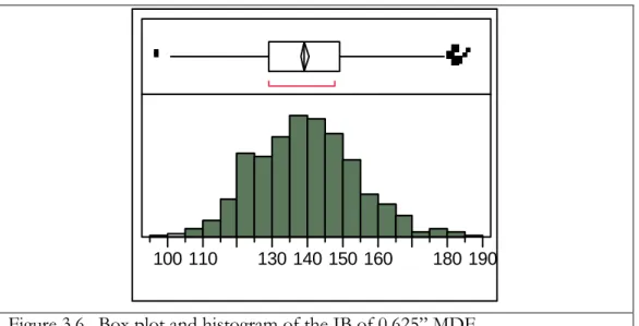
Figure 3.6. Box plot and histogram of the IB of 0.625” MDF……… 56
Figure 3.7. Normal probability plot of the IB of 0.625” MDF……… 56
Figure 3.8. Log Normal probability plot of the IB of 0.625” MDF………. 57
Figure 3.9. Box plot and histogram of the IB of 0.750” MDF……… 57
Figure 3.10. Normal probability plot of the IB of 0.750” MDF………. 58
Figure 3.11. Logistic probability plot of the IB of 0.750” MDF……… 58
List of Figures
(continued)
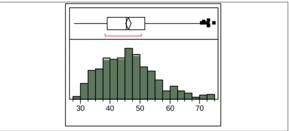
Page Figure 3.13. Log Normal probability plot of the IB of OSB………59 Figure 3.14. Largest Extreme Value probability plot of the IB of OSB………. 60 Figure 3.15. Box plot and histogram of the Parallel EI of OSB……….. 60 Figure 3.16. Largest Extreme Value probability plot of the Parallel EI of OSB…….. 61 Figure 3.17. Log Logistic probability plot of the Parallel EI of OSB……… 61
Appendix to Chapter IV
Figure 4.1. Comparison of Adjusted R2 and AIC for first-order stepwise regression
models for MDF 0.500” for every record length greater than 50……. 91 Figure 4.2. Comparison of Adjusted R2 and AIC for first-order stepwise regression
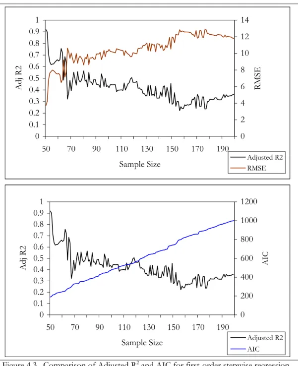
models for MDF 0.625” for every record length greater than 50……. 92 Figure 4.3. Comparison of Adjusted R2 and AIC for first-order stepwise regression
models for MDF 0.750” for every record length greater than 50……. 93 Figure 4.4. Residuals by predicted IB plot for the second-order model,
MDF 0.500”, n=60……….. 94 Figure 4.5. Time series graph of validation data set for the second-order model,
MDF 0.500”, n=15………. 94 Figure 4.6. XY scatter plot of training (top) and validation (bottom)
data sets for the second-order model, MDF 0.500”, n=60………….. 95 Figure 4.7. Prediction profiles for the second-order model, MDF 0.500”, n=60…… 96 Figure 4.8. Response surface plots of IB for: “fFaceMstM” and “hPrCls2Tim”
(upper left); “eBoilrStmP” and “fFaceMstM” (upper right); “dCoreTemp” and “fFaceMstM” (lower left); and “dCoreTemp” and “aChipAugSp” (lower right) for the second-order model,
MDF 0.500”, n=60……… 96 Figure 4.9. Residuals by predicted IB plot for the first-order model,
List of Figures
(continued)
Page Figure 4.10. Time series graph of validation data set for the first-order model,
MDF 0.500”, n=33……… 97 Figure 4.11. XY scatter plot of training (top) and validation (bottom)
data sets for the first-order model, MDF 0.500”, n=175……… 98 Figure 4.12. Prediction profiles for the first-order model, MDF 0.500”, n=175…… 99 Figure 4.13. Residuals by predicted IB plot for the first-order model for
MDF 0.625”, n=62……… 99 Figure 4.14. Time series graph of validation data set for the first-order model
for MDF 0.625”, n=13……….. 100 Figure 4.15. XY scatter plot of training data set (top) and validation (bottom)
data set for the first-order model for MDF 0.625”, n=62…………. 101 Figure 4.16. Prediction profiles the first-order model for MDF 0.625”, n=62…... 102 Figure 4.17. Response surface plot of IB for “gPreBBSpd” and “cC00046”
for the first-order model for MDF 0.625”, n=62.
(grid-line 120 p.s.i.)………. 102 Figure 4.18. Residual by predicted IB plot for the second-order model for
MDF 0.625”, n=400………... 103 Figure 4.19. Time series graph of validation data set for the second-order model
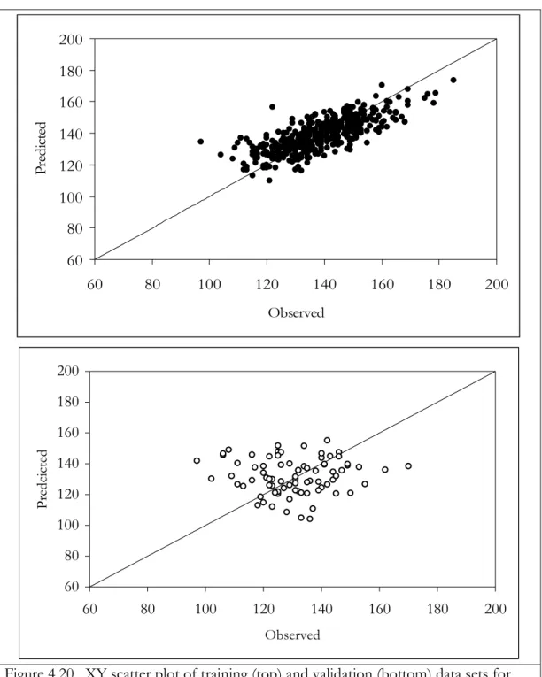
for MDF 0.625”, n=80………... 103 Figure 4.20. XY scatter plot of training (top) and validation (bottom)
data sets for the second-order model for MDF 0.625”, n=400…….. 104 Figure 4.21. Prediction profiles for the second-order model for
MDF 0.625”, n=400………... 105 Figure 4.22. Response surface plot of IB for “hPrPPMTimS” and “fCoreHTmpT”
for the second-order model for MDF 0.625”, n=400………. 105 Figure 4.23. Residual by predicted IB plot for the second-order model for
List of Figures
(continued)
Page Figure 4.24. Time series graph of validation data set for the second-order model
for MDF 0.750”, n=15………... 106 Figure 4.25. XY scatter plot of training (top) and validation (bottom)
data sets for the second-order model for MDF 0.750”, n=70………. 107 Figure 4.26. Prediction profiles for the second-order model for MDF 0.750”, n=70.. 108 Figure 4.27. Response surface plot of IB for “fFaceMstm” and “dCoreScvWR”
(left) and for “hPrOpnTime” and “dCoreScvWR” (right) for
the second-order model for MDF 0.750”, n=70……….. 108 Figure 4.28. Residual by plot for the second-order model with interaction terms,
MDF 0.750”, n=200………109 Figure 4.29. Time series graph of validation data set for the second-order model
with interaction terms, MDF 0.750”, n=40………... 109 Figure 4.30. XY scatter plot of training (top) and validation (bottom)
data sets for the second-order model with interaction terms,
MDF 0.750”, n=200……….... 110 Figure 4.31. Comparison of Adjusted R2 and RMSE (upper) and Adjusted R2 and
AIC (lower) for first-order models for OSB IB for every record
length greater than 50………..111 Figure 4.32. Comparison of Adjusted R2 and RMSE (upper) and Adjusted R2 and
AIC (lower) for first-order models for OSB Parallel EI for every
record length greater than 50……….. 112 Figure 4.33. Residual by predicted IB plot for the second-order model with
Box Cox transform, OSB IB, n=59………. 113 Figure 4.34. Time series graph of validation data set for the second-order model
with Box Cox transform, OSB IB, n=12………. 113 Figure 4.35. XY scatter plot of training (top) and validation (bottom)
data sets for the second-order model with Box Cox transform,
OSB IB, n=59……… 114 Figure 4.36. Prediction profiles for the second-order model with Box Cox transform,
List of Figures
(continued)
Page Figure 4.37. Response surface plots of OSB Parallel EI for: “Dry2Out” and
“BnkSpdTCL” (upper left); “MTCLMoiLev” and “Dry2Out” (upper right); “MTCLMoiLev” and “BunkerSpdTCL” (lower left); and “Dr3OutMois” and “MTCLMoiLev” (lower right) for the
second-order model with Box Cox transform, OSB IB, n=59……… 116 Figure 4.38. Residual by plot for the second-order model with Box Cox
transform, OSB IB, n=300……….. 117 Figure 4.39. Time series graph of validation data set for the second-order model
with Box Cox transform, OSB IB, n=60………. 117 Figure 4.40. XY scatter plot of training (top) and validation (bottom)
data sets for the second-order model with Box Cox transform,
OSB IB, n=300………... 118 Figure 4.41. Residual by predicted Parallel EI plot for the first-order model,
OSB Parallel EI, n=58……… 119 Figure 4.42. Time series graph of validation data set for the first-order model,
OSB Parallel EI, n=16……… 119 Figure 4.43. XY scatter plot of training (top) and validation (bottom)
data sets for the first-order model, OSB Parallel EI, n=58………….. 120
Appendix to Chapter V
Figure 5.1. Histograms and quantile plots of “Core fiber humidifier temperature” (left) and “Swing refiner separator outlet pressure” (right) for
0.625” MDF, n=400………... 145 Figure 5.2. Linear and regression fits for IB to the sub-spaces of
“Swing refiner separator outlet pressure” for 0.625” MDF, n=400 (blue line fits the blue points; red line fits the red points; black line fits all of the data)………... 146 Figure 5.3. RMSEP by record length and modeling type for 0.500” MDF IB……... 147 Figure 5.4. RMSEP by record length and modeling type for 0.625” MDF IB………. 147 Figure 5.5. RMSEP by record length and modeling type for 0.750” MDF IB………. 148
List of Figures
(continued)
Page Figure 5.6. RMSEP by record length and modeling type for the IB of OSB……….. 148 Figure 5.7. RMSEP by record length and modeling type for the Parallel EI of OSB.. 149 Figure 5.8. Quantile third-order RT model with v-fold
v-fold cross-validation for 0.500” MDF, n=100.………. 150 Figure 5.9. XY scatter plot of training (top) and validation (bottom) data sets
for the third-order quantile regression RT model
with v-fold cross-validation node pruning for 0.500” MDF,
n=100……… 151 Figure 5.10. XY scatter plot of training (top) and validation (bottom) data sets
for the stepwise regression RT model with v-fold cross-validation node pruning for 0.500” MDF, n=175……… 152 Figure 5.11. Time series graph of validation set for the stepwise regression RT
model with v-fold cross-validation node pruning for 0.500” MDF, n=35………... 153 Figure 5.12. Time series graph of validation data set for the second-order RT
model without node pruning for 0.500” MDF, n=13……….. 153 Figure 5.13. XY scatter plot of training (top) and validation (bottom) data sets for
the second-order RT model without node pruning for 0.500”
MDF, n=60………. 154 Figure 5.14. RT and mixed stepwise regression equations for 0.625” MDF, n=200… 155 Figure 5.15. Time series graph of validation data set for the multiple linear quantile
RT model with v-fold cross-validation node pruning for 0.625”
MDF, n=300……….. 155 Figure 5.16. XY scatter plot of training (top) and validation (bottom) data sets
for the multiple linear quantile RT model with v-fold cross-validation node pruning for 0.625” MDF, n=300……… 156 Figure 5.17. Piecewise simple linear model with v-fold cross-validation node pruning
List of Figures
(continued)
Page Figure 5.18. Time series graph of validation data set for the piecewise simple
linear model with v-fold cross-validation node pruning for 0.625”
MDF, n=400………... 158 Figure 5.19. XY scatter plot of training (top) and validation (bottom)
data sets for the piecewise simple linear model with v-fold
cross-validation node pruning for 0.625” MDF, n=400……….. 159 Figure 5.20. XY scatter plot of training (top) and validation (bottom)
data sets for the second-order RT model with
v-fold cross-validation node pruning for 0.625” MDF, n=62……….. 160 Figure 5.21. Time series graph of validation data set for the second-order
RT model with v-fold cross-validation node
pruning for 0.625” MDF, n=13……….. 161 Figure 5.22. Time series graph of validation data set for the multiple linear
quantile RT model without node pruning for 0.750” MDF, n=100… 161 Figure 5.23. Multiple linear quantile RT model without node pruning for 0.750”
MDF, n=100……….. 162 Figure 5.24. XY scatter plot of training (top) and validation (bottom) data sets
for the multiple linear quantile RT model without node pruning
for 0.750” MDF, n=100……….. 164 Figure 5.25. Time series graph of validation data set for the piecewise simple
linear RT model without node pruning for 0.750” MDF, n=200……. 165 Figure 5.26. XY scatter plot of training (top) and validation (bottom) data sets
for the piecewise simple linear RT model without node pruning
for 0.750” MDF, n=200……….. 166 Figure 5.27. XY scatter plot of training (top) and validation (bottom) data sets
for the second-order RT model with v-fold
v-fold cross-validation for 0.750” MDF, n=70……… 167 Figure 5.28. Time series graph of validation data set for the second-order
RT model with v-fold cross-validation for 0.750”
List of Figures
(continued)
Page Figure 5.29. Time series graph of validation data set for the mixed stepwise
all possible subsets RT model without node pruning for the
IB of OSB, n=100………. 168 Figure 5.30. XY scatter plot of training (top) and validation data sets (bottom)
for the mixed stepwise all possible subsets RT model without
node pruning for the IB of OSB, n=100……… 169 Figure 5.31. Time series graph of validation data set for the mixed stepwise
all possible subsets RT model without node pruning for the
IB of OSB, n=200………. 170 Figure 5.32. XY scatter plot of training (top) and validation data sets (bottom)
for the mixed stepwise all possible subsets RT model without
node pruning for the IB of OSB, n=200………. 171 Figure 5.33. Time series graph of validation data set for the mixed stepwise
all possible subsets RT model without node pruning for the
IB of OSB, n=300………. 172 Figure 5.34. XY scatter plot of training (top) and validation (bottom) data sets
for the mixed stepwise all possible subsets RT model without
node pruning for the IB of OSB, n=300……… 173 Figure 5.35. XY scatter plot of training (top) and validation (bottom) data sets
for the second-order RT model without node pruning
for the IB of OSB, n=59………. 174 Figure 5.36. Time series graph of validation data set for the second-order
RT model without node pruning for the IB of
OSB, n=12………. 175 Figure 5.37. Time series graph of validation data set (lagged one time period)
for the third-order RT model without node pruning
for the Parallel EI of OSB, n=21……….. 175 Figure 5.38. XY scatter plot of training (top) and validation data sets (bottom)
for the third-order RT model without node pruning
List of Figures
(continued)
Page Figure 5.39. Time series graph of validation data set for the third-order
RT model without node pruning for the Parallel EI
of OSB, n=200……….... 177 Figure 5.40. XY scatter plot of training (top) and validation (bottom) data sets
for the third-order RT model without node pruning
for the Parallel EI of OSB, n=200……….. 178 Figure 5.41. XY scatter plot of training (top) and validation (bottom) data sets
for the second-order RT model without node pruning
for the Parallel EI of OSB, n=58………. 179 Figure 5.42. Time series graph of validation data set (lagged one time period)
for the second-order RT model without node pruning
for the Parallel EI of OSB, n=58………. 180 Figure 5.43. RMSEP for RT and MLR models discussed in Chapters IV and V…… 181
Appendix to Chapter VI
Figure 6.1. Comparison of RMSEP with and without Box Cox transform for all RT models analyzed for OSB IB (yellow bars indicate best
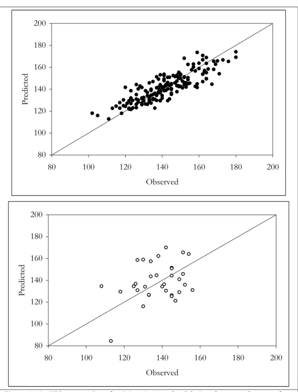
candidate models discussed in this chapter)……… 191 Figure 6.2. Second-order model for OSB IB (n=59) with Box Cox transformation.... 192 Figure 6.3. XY scatter plots of predicted and observed IB for OSB IB (n=59)
without Box Cox transform (top graph) and with Box Cox
transform (bottom graph)……….... 193 Figure 6.4. XY scatter plot of validation data sets for OSB IB (n=59) without
Box Cox transform (top graph) and with Box Cox transform
(bottom graph)……… 194 Figure 6.5. Time series graph of validation data sets for OSB IB (n=59) without
Box Cox transform (top graph) and with Box Cox transform
(bottom graph)……… 195 Figure 6.6. XY scatter plot (top graph) and time series graph (bottom graph) of
List of Figures
(continued)
Page Figure 6.7. Illustration of regression model differences for “main forming line total
weight” in node one of RT model for OSB IB (n=59)……… 197
Figure 6.8. XY scatter plots of predicted and observed IB for OSB IB (n=100) without Box Cox transform (top graph) and with Box Cox
transform (bottom graph)………198
Figure 6.9. XY scatter plot of validation data sets for OSB IB (n=100) without Box Cox transform (top graph) and with Box Cox
transform (bottom graph)………199 Figure 6.10. Time series graph of validation data sets for OSB IB (n=100)
without Box Cox transform (top graph) and with Box Cox
transform (bottom graph)………200
Figure 6.11. XY scatter plots of predicted and observed IB for OSB IB (n=200) without Box Cox transform (top graph) and with
Box Cox transform (bottom graph)………201
Figure 6.12. XY scatter plot of validation data sets for OSB IB (n=200) without Box Cox transform (top graph) and with Box Cox
transform (bottom graph)………... 202 Figure 6.13. Time series graph of validation data sets for OSB IB (n=200)
without Box Cox transform (top graph) and with Box Cox
transform (bottom graph)……….. 203
Figure 6.14. XY scatter plots of predicted and observed IB for OSB IB (n=300) without Box Cox transform (top graph) and with
Box Cox transform (bottom graph)………... 204
Figure 6.15. XY scatter plot of validation data sets for OSB IB (n=300) without Box Cox transform (top graph) and with Box Cox
transform (bottom graph)………205 Figure 6.16. Time series graph of validation data sets for OSB IB (n=300)
without Box Cox transform (top graph) and with Box Cox
CHAPTER I. INTRODUCTION
An underlying basis of statistical methods is the study of variance (σ2). Variance
in the context of manufacturing is defined as estimated process variance (σˆ2). In forest
products manufacturing, process variance results in inferior product quality, poor product safety and noncompetitive costs. Process variance is masked by higher than necessary operational targets (e.g., weight, thickness, density, resin, etc.) which require higher than necessary energy use which in combination are not competitive or sustainable in a highly competitive market place.
A common goal for statistical research is to investigate and quantify causality between independent variables (X) and response variables (Y) with a high level of scientific inference. As Friedman (2001) notes, given a set of measured values of attributes,
characteristics or properties on a object (observation) X = (X1, X2, …. Xn), which are
often called “variables,” the goal is to predict (estimate) the unknown value of another attribute Y. In quantifying causality, de Mast and Trip (2007) note the important distinction between exploratory and confirmatory data analysis which they attribute to Tukey’s (1977) work. As Tukey (1977) pointed out, confirmatory data analysis is
concerned with testing a pre-specified hypothesis. The purpose of exploratory data analysis is hypothesis generation (de Mast and Trip 2007). This dissertation is undertaken in the spirit of exploratory data analysis and hypothesis generation. The dissertation is aligned with Gleser’s (1996) “First Law of Applied Statistics,” i.e., two individuals using the same statistical method on the same data should arrive at the same conclusion.
The goal of the dissertation is to improve the understanding of causality for the strength properties of MDF and OSB from industrial derived data. The dissertation is focused on exploratory analysis in the context of data mining, i.e., quantifying unknown causality from large volumes of electronically collected data which are fused with destructive data of strength properties.
Data mining (DM), also called Knowledge-Discovery in Databases (KDD) or Knowledge-Discovery and Data Mining, is the process of automatically searching large volumes of data for patterns (http://en.wikipedia.org/wiki/Data_mining. referenced
10/4/07). DM is the contemporary edge of the sciences of Artificial Intelligence, Machine Learning, Pattern Recognition and Data Visualization. DM evolved from advancements in database management systems (DBMS) and on-line (real-time) transaction processing (OLTP). From a statistical perspective it can be viewed as computer automated exploratory data analysis of large complex data sets (Friedman and Wall 2005).
Exponential growth of data mining applications has occurred globally for many industries (Harding et al. 2006). Rapid growth in data mining applications in the forest products industry is imminent and is desperately needed for the industry’s economic survival.
The New Millennium for the Forest Products Industry
Forests sustain an important forest products economy in the U.S. and state of Tennessee. The forest products industry contributed more than $240 billion to the U.S. economy and employed more than 1,000,000 Americans in 2002 (U.S. Census Bureau 2004). Over 180,000 Tennesseans were employed by the forest products industry in 2000 accounting for 6.6 percent of Tennessee’s economy by generating $21.7 billion in value in
that same year (Young et al. 2007). Threats to this economic sector have arisen in the form of unprecedented levels of international competition, constrained credit markets, increasing fiber costs, increasing energy costs and substitution from renewable wood products to non-renewable oil- and cement-derived products.1
Wood costs represent the largest single component of total manufacturing costs for most forest products manufacturers. Some U.S. manufacturers must contend with wood costs as high as 60% of total manufacturing costs.2 Demand/capacity ratios for the
engineered wood panel sector are falling below the critical threshold of 85 percent, a level that results in declining real prices. A renewed emphasis on reducing costs is desperately needed by this important economic sector.
Rationale and Justification
Poor production efficiencies in the engineered wood panel sector occur from
unacceptably high levels of wood waste due to low strength and high wood-density targets. Poor production efficiencies lead to high wood use, high energy usage, and an overall lack of business competitiveness. Wood waste is a significant contributor to costs. In 2003, the engineered wood panel sector produced 64.3 billion square feet of panels and wood waste ranged from three percent to nine percent (Composite Panel Association 2004, TECO 2004). Reducing wood waste by one percent could translate into annual savings of as much as $700,000 per producer and promote wiser use of the forest resource.3
1U.S. structural wood panel mills lost 5.8 percent of the North American market in 2004, primarily
from Europe and South America. Imports over the long term are forecast to increase (Engineered Wood Association 2004).
2Personal communications 2005 and 2006: Georgia-Pacific, J.M. Huber Corporation,
Louisiana-Pacific Corporation, Norbord Corporation and Weyerhaeuser Corporations.
Louisiana-Improved production efficiencies, reduced wood waste, and lower costs are possible from data mining by improving the knowledge of causality of sources of unknown process variation.
Many organizations can be labeled as “data-rich” and “knowledge-poor” (Chen 2005). Modeling of wood composite manufacturing processes enables complex processes to be better understood by examining the patterns in data related to the previous behavior of a manufacturing process (Young and Guess 2002). The benefits of first-order models in engineered wood panel production are well documented (Young 1997, Gruebel 1999, Bernardy and Scherff 1998, 1999, Erilsson et al. 2000, Young and Guess 2002, Guess et al. 2003, and Kim et al. 2007). Erilsson et al. (2000) discussed the potential of stochastic models for engineered wood manufacture, while Gruebel (1999) documented medium density fiberboard (MDF) manufacturing cost savings of five percent to ten percent from the use of “off-line” first-order statistical models. Dawson et al. (2006) developed a genetic algorithm/neural network (GANN) real-time predictive model of MDF and oriented strand board (OSB) manufacturing processes that resulted in cost annual savings at two test sites ranging from $700,000 to $1.2 million.
This dissertation investigates the use of Regression Tree (RT) models to identify unknown causality between process variables and strength properties of wood composites.
RT models are known for their high explanatory value and RT models are at least as
predictive as black box deterministic methods (Loh 2002).
Problem Statement and Scope
The problem statement of this dissertation is to explore the explanatory and predictive capabilities of parametric and non-parametric (quantile) regression tree models
of the strength properties of MDF and OSB using real-time sensor data amassed in manufacturers’ data warehouses. Specifically, this research will investigate the explanatory and predictive capabilities of three modeling methods: first-, second- and third-order statistical multiple linear regression models with interaction terms, parametric regression trees, and non-parametric (quantile) regression trees. The models are developed for one MDF and one OSB mill both located in the southeastern United States.
Dissertation Hypothesis
The null research hypothesis of this dissertation is that there is no significant difference in the explanatory or predictive capabilities of three modeling methods: first-, second- and third-order statistical multiple linear regression models with interaction terms; parametric regression trees; and non-parametric (quantile) regression trees. The test of this research hypothesis hopefully will incrementally advance the statistical and industrial engineering sciences as applied to wood composites manufacture.
Dissertation Objectives
1. Investigate first-, second- and third-order MLR models
First-, second- and third-order MLR models with interaction terms are investigated for MDF and OSB wood composite strength properties. The database to support this work is the real-time relation database developed by Young and Guess (2002), enhanced by Dawson et al. (2006). MLR models are developed for three predominately
manufactured products (0.500”, 0.625” and 0.750” industrial grades) for MDF and one OSB product (7/16” roof sheathing) for each test site.
2. Investigate regression tree (RT) models
Parametric and non-parametric (quantile) regression trees (RT) are investigated for each MDF and OSB manufacturing test site. The same database of the first objective is used. RT models are developed for the same nominally produced MDF and OSB products defined in the first objective.
3. Compare the explanatory and predictive capabilities of the MLR and RT models
developed in the first and second objectives.
The explanatory and predictive capabilities of the MLR and RT models developed in the first and second objectives are compared. Model prediction capabilities are analyzed for appropriate validation data sets from each MDF and OSB mill.
There is no documentation in the literature of the investigation and application of decision tree theory to manufactured wood composites strength properties. It is hoped that this research will at least incrementally expand the sciences of wood composites manufacture and decision tree theory.
The dissertation is organized in seven chapters. In Chapter II the relevant
literature for the dissertation is reviewed. The methods used in the research are presented in Chapter III, with a description of the data and an assessment of the data quality
(descriptive statistics and distribution fits) for the important response variables. The results of the first objective are given in Chapter IV. Chapter V is the core chapter of the dissertation where results are presented on regression trees. Chapter VI compares the results of the first two objectives. Chapter VII summarizes the dissertation with conclusions and a discussion of future research. The Bibliography and General Appendices follow Chapter VII.
CHAPTER II. LITERATURE REVIEW
Information technology is the largest single capital investment for many enterprises (Thorpe 1998). However, many companies struggle with making use of the vast amount of data that is acquired at increasingly faster rates. Thorpe (1998) called this phenomenon the “Information Paradox” where companies invest increasing amounts of money on information acquisition but cannot demonstrate a connection between the money spent and business results. This paradox is caused from the lack of useful “real-time relational databases” that are of sufficient design and organization where parametric and non-parametric statistical methods can be used to investigate unknown causality and develop scientific knowledge. The data warehouse in many ways is the nucleus for process knowledge of a manufacturing enterprise. As Harding et al. (2006) noted, “Knowledge is the most valuable asset of a manufacturing enterprise, as it enables a business to
differentiate itself from competitors and to compete efficiently and effectively to the best of its ability.” The Harding et al. (2006) statement is very appropriate for the wood composites industry in the present era of unprecedented competition, increasing raw material costs, increasing energy costs and declining product prices.
Data Warehouse
As Inmom and Hackathorn (1994) noted, a data warehouse is the main repository of the organization's historical data, its corporate memory.4 The central concept of a data
4The origin of the data warehouse can be traced to studies at MIT in the 1970s which were targeted at developing an optimal technical architecture. At the time, the craft of data processing
warehouse is that it is a collection of records. Data warehouses usually consist of one or more databases of volumes of records. The structure of a database is known as a schema. The schema describes the objects that are represented in the database and the table
relationships among them. Multiple related tables each consisting of rows and columns is the most common form of schema (White 2002). Schema design is a critical factor in ensuring optimal storage and data compression, and also ensures the overall usefulness of the data during retrieval for analysis.
Real-time Data Warehouse
Real-time data warehousing originated and evolved with the computer industry. Real-time data captures manufacturing activity as it occurs. Real-time data usually are stored in a data warehouse either at the occurrence of an event or as a function of time. Most real-time data warehouse platforms can efficiently store multiple gigabytes of process data. Real-time data warehousing has become affordable in the last decade and it is hard to find a modern forest products manufacturer that does not have some type of real-time data warehousing platform. However, most forest products manufacturers use real-time data for simple trending analysis and rudimentary process knowledge. They struggle with using real-time databases for advanced analytics and scientific knowledge of the process. This dissertation directly addresses improved scientific knowledge of processes from the use of parametric and non-parametric regression tree methods using real-time process data.
Real-time databases have inherent data storage characteristics that need to be understood before advanced analytics can occur. Data quality is a key obstacle in the use
of real-time data storage. Real-time data quality problems such as null fields, repeated records, correct time stamps, bi-modality/multi-modality and data leverage are significant issues which confound advanced analytics and data mining efforts. Some research has addressed data quality issues during real-time data retrieval using first-order statistical models and deterministic algorithms (e.g., genetic algorithms and neural networks) to model the wood composite process (Gruebel 1999; Bernardy and Scherff 1998, 1999; Young et al. 2004 and Dawson et al. 2006). The key first step in the use of real-time data is the development of the real-time relational database.
Real-time Relational Database
A real-time relational database is defined as the alignment of real-time process sensor data from the production line with product quality data, e.g., destructive test data of strength quality developed from the mill testing laboratory. The real-time relational
database used in this dissertation is considered to be distributed data fusion (also called track-to-track fusion) where data from multiple diverse sensors are combined in order to make inferences about a physical event, activity or situation, e.g., internal bond tensile strength, modulus of elasticity flexure strength, etc. (Hall 1992).5 Intellectual latency is the
most significant issue in real-time relational databases. Some intellectual latency results from improper time alignment of process sensor data with product quality data. Young and Guess (2002) developed an automated relational database that addressed some of the issues of intellectual latency. Clapp et al. (2007) use the Eigenvalues from principal
5 Data fusion or information fusion are names that have been given to a variety of interrelated
expert system problems which have arisen primarily in military applications (Goodman et al. 1997). Other applications of data fusion include remote sensing, medical diagnostics and robotics
component analysis to identify improper time alignment of real-time process sensors with destructive test data for MDF.
A data warehouse or real-time data warehouse contains just data. The key to scientific inference and improvement is the conversion of information or data into knowledge. This dissertation attempts to advance the scientific understanding of MDF and OSB manufacture. Many forest products manufacturers are unsuccessful in the information-to-knowledge transformation because they lack the key foundation of an automated real-time relational database.
Data Mining
Data mining (DM) is used to discover patterns and relationships in data, with an emphasis on large observational databases (Friedman and Wall 2005). DM is a large discipline and a plethora of literature exists on the subject. The literature review of DM in this chapter is not intended to be comprehensive, but instead a helpful precursor for the analytical methods used in this dissertation.
DM is the contemporary edge of the sciences of Artificial Intelligence, Machine Learning, Pattern Recognition and Data Visualization. DM evolved from advances in database management systems (DBMS) and on-line (real-time) transaction processing (OLTP). From a statistical perspective it can be viewed as computer automated exploratory data analysis of large complex data sets (Friedman 2001). DM is directly related to the field of Decision Theory. As Friedman (2001) notes, “It also affords enormous research opportunities for new methodological developments… ….Statistics can potentially have a major influence on Data Mining.”
DM is closely related to machine learning and prediction. The predictive or machine learning problem is easy to state if difficult to solve in general (Friedman 2001). Given a set of measured values of attributes, characteristics or properties, on a object (observation) X = (X1, X2, …. Xn), which are often called “variables,” the goal is to predict (estimate) the unknown value of another attribute Y (Friedman 2001). The quantity Y is called the “output,” “dependent” or “response” variable, and X = (X1, X2, …. Xn) are referred to as the “input,” “independent,” “predictor” or "regressor” variables
(Friedman 2001). The prediction takes the form of a function Yˆ=F x x( ,1 2,... )xn =F x( ) that maps a point X in the space of all joint values of the predictor variables, to a point
ˆ
Yin the space of response values (Friedman 2001). Most scientists agree that the goal is to produce a “good” predictive F(x).
Decision trees are one of the most popular predictive learning methods used in data mining. Decision trees were developed largely in response to the limitations of kernel methods (Friedman 2001).6 No matter how high the dimensionality of the predictor
variable space, or how many variables are actually used for prediction (splits), the entire model can be represented by a two-dimensional graphic, which can be plotted and easily interpreted (Friedman 2001). Decision trees have an advantage of being very resistant to irrelevant predictor or regressor variables, i.e., since the recursive tree building algorithm estimates the optimal variable on which to split at each step, regressors unrelated to the response tend not to be chosen for splitting (Breiman et al. 1984). Friedman (2001) also
6Kernel Methods (KMs) are a class of algorithms for pattern analysis, whose best known element
is the Support Vector Machine (SVM). Support vector machines (SVMs) are a set of related supervised learning methods used for classification and regression. They belong to a family of generalized linear classifiers. The general task of pattern analysis is to find and study general types of relations (for example clusters, rankings, principal components, correlations, classifications) in
notes a strength of decision trees is that regressors do not have to be tuned (standardized) which makes the method an “off-the-shelf” procedure. Fore example, NIR spectral data have been used with decision trees to enhance automated classifications of fruit and organic matter in soil (Ware et al. 2001, Shepherd and Walsh 2002, Shepherd et al. 2003).
This ease of interpretation from two-dimensional plots makes decision trees a powerful tool for the practitioner and an appropriate methodology for this dissertation for ease of use by practitioner. Fitting quotes supportive of this dissertation are by C. Dickens and J.H. Friedman (Friedman 1994), “Every time computing power increases by a factor of ten we should totally rethink how we compute.” Friedman’s (2001) corollary, “Every time the amount of data increases by a factor of ten, we should totally rethink how and what we compute.” A more detailed literature review of decision trees is presented later in this chapter.
Multiple Linear Regression
The method of least squares and the precursor to regression analysis can be dated to 1805 by the publication of Legendre’s work on the subject (Stigler 1986). Sir Francis Galton discovered regression around 1885 in studies of heredity (Stigler 1986). Galton’s regression (as finally developed by Yule) was not simply an adaptation of least squares to a different set of problems; it was a new way of thinking about multivariate data (Stigler 1986).
Today regression analysis remains one of the most popular and globally used tools. Practitioners like regression analysis because of ease of interpretation in the coefficients that do not require standardization of the data of either the dependent and independent variables. Practitioners also like the visual interpretation of regression. Simple linear (SL)
and multiple linear regression (MLR) methods are widely available on business and
statistical software, and MLR is a prerequisite for most undergraduate business and science degrees.
For situations where the data are drawn from reasonably homogeneous populations, traditional methods such as MLR can yield insightful analyses. The usefulness of MLR in data mining can breakdown quickly if the stringent assumptions associated with MLR are not met, e.g., normality assumption of the response (Y).
There is a plethora of literature on regression analysis and many tomes are available on the method. An extensive literature review of the heavily referenced MLR method is not presented in this dissertation given that it is not the primary method used for analysis.
Quantile Regression
As noted by Koenker (2005), Edgeworth’s (1888) work on median methods is the genesis of the idea of quantile regression. Edgeworth emphasize that the assumed
optimality of the sample mean as an estimator of location was crucially dependent on the assumption that the observations came from a common normal distribution. If the observations departed from normals with different variances, the median, Edgeworth argued, could easily be superior to the mean. Koenker (2005) notes that Edgeworth (1888) discards the Boscovich-Laplace constraint related to least squares that the residuals sum to zero and proposes to minimize the sum of the absolute residuals in both slope and
intercept parameters. Unfortunately, the computational rigors associated with
Edgeworth’s (1888) work limited the application of the method until the development of linear programming which provides an efficient conceptual approach. Mosteller (1946)
discovered that quantile estimators are almost as efficient as the maximum likelihood estimators for most conventional parametric models.
Quantile regression as introduced by Koenker and Bassett (1978) seeks to extend these ideas to the estimation of conditional quantile function, i.e., models in which
quantiles of the conditional distribution of the response variable are expressed as functions of observed covariates. The quantile regression literature in economics makes a persuasive case for the value of going beyond models for the conditional mean (Chamberlain 1994). Koenker and Billias (2001) explore quantile regression models for unemployment duration data and offer an introduction to quantile regression for demand analysis. There is also a growing literature database in empirical finance employing quantile regression methods. Bassett and Chen (2001) consider quantile regression index models to characterize mutual fund investment styles. Shaffer (2007) and Young et al. (2007c) explore the first uses of quantile regression in modeling the internal bond strength property of MDF. The method of quantile regression is described in more detail in the next chapter.
Decision Trees
The machine learning technique for inducing a decision tree from data is called decision tree learning, or (colloquially) “decision trees”.7 Decision tree (DT) models have
grown into a powerful class of methods for examining complex relationships with many types of data (Kim et al. 2007). Researchers and practitioners find great explanatory value in DT models. DT models are more useful than MLR models when data are not
homogeneous (Figure 2.1).
A “regression tree” is a decision tree for numerical data. A “classification” tree is a decision tree for categorical data. Since this dissertation uses numerical data from
industrial processes, the primary focus of the following literature review is for the regression tree (RT).
A regression tree is a piecewise constant or piecewise linear estimate of a
regression function, constructed by recursively partitioning the data and sample space. Its name derives from the practice of displaying the partitions as a decision tree, from which the roles of the regressors are inferred (Figure 2.2).
Construction of a regression tree consists of the following general steps performed iteratively, ending with step four:
à Partition the data,
à Fit a model to the data in each partition,
à Stop when the residuals of the model are near zero or a small fraction of observations are left,
à Prune the tree if it over fits.
Most of the contemporary regression tree algorithms differ on steps one and two. Many popular graphical-user interface software packages that have DT algorithms do not have step four (e.g., JMP - http://www.jmp.com/, Statistica - http://www.statsoft.com/, etc., referenced 10/5/07).
The AID (“Automatic Interaction Detection”) algorithm by Morgan and Sunquist (1963), Kass (1975) and Fielding (1977) is the first implementations of the DT idea. AID searches over all axis-orthogonal partitions and yields a piecewise constant estimate (Loh 2002). At each stage, the partition that minimizes the total sums of squared errors (SSE) is selected. Splitting stops if the fractional decrease in total SSE is less than a pre-specified γ or if the sample size is too small. As noted by Loh (2002), a weakness of AID is that it is
hard to specify γ, i.e., too small or too large a γ leads to over- or under-fitting. Another weakness of AID (Doyle 1973) is that the “greedy search” approach induces a bias in variable selection, e.g., if X1 and X2 are ordered regressors with n1 > n2, X1 will have a higher chance of being selected which leads to erroneous inferences from the final tree structure. “Greedy search” methods find the regressor that minimizes the total SSE in the regression models fitted to the data subsets defined by the split (e.g., JMP and Statistica). “Greedy search” methods are also computationally expensive (Loh 2002).
The CART© (“Classification and Regression Trees”, http://www.salford-systems.com/
referenced 9/20/07) algorithm followed AID and is a popular DT method (Breiman et al. 1984). Unlike AID, it avoids choosing a γ by employing a backward-elimination strategy to determine the tree (Loh 2002). It grows an overly large tree and then prunes away some branches, using a test sample or v-fold cross-validation (CV) to estimate the total SSE. In step two of the four general steps of decision trees, the CART regression tree fits a mean function in each partition (also called a piecewise constant regression tree).
The MARS© (“Multivariate Adaptive Regression Splines”) by Friedman (1991,
http://www.salford-systems.com/ referenced 9/20/07) method combines spline fitting with recursive partitioning to produce a continuous regression function estimate
(Chaudhuri et al. 1995). Chaudhuri at al. (1995) note that the complexity of the estimate from MARS© makes interpretation difficult and theoretical analysis of the spline statistical properties extremely challenging.
Quinlan's (1992) M5 method constructs an ordinary regression tree with a stepwise linear regression model fitted to each node at every stage. As noted in Kim et al. (2007b), Chaudhuri et al. (1994) chose a residual-based approach from MLR models. This
approach selects the variable with the signs of the residuals which appear most non-random, as determined by the significance probabilities of two-sample t-tests.
The FIRM algorithm (“Formal Inference-based Recursive Modeling”) by Hawkins (1997) addresses the bias problem of AID by using Bonferroni-adjusted significance tests to select predictors for splitting. Unlike AID and CART, FIRM splits each node into as many as ten subnodes for an ordered regressor. As Loh (2002) noted from Hawkins (1997) work, the Bonferroni adjustment can over-correct, resulting in a bias toward regressors that have fewer splits.
As cited by Loh (2002), other methods have been proposed for determining the final tree: Ciampi et al. (1988, 1991) combine non-adjacent partitions; Chaudhuri et al. (1994) use a CV-based, look-ahead procedure; Marshall (1995) finds non-hierarchical partitions; Chipman et al. (1998) and Denison et al. (1998) employ Bayesian methods to search among trees; and Li et al. (2000) use a stopping rule based on statistical significance tests.
The GUIDE, ver. 5.2 (“Generalized, Unbiased, Interaction Detection and Estimation”) DT algorithm is used in this research. GUIDE (Loh 2002, Chaudhuri and Loh 2002) extend the idea of Chaudhuri et al. (1994) by means of “curvature tests”
(www.stat.wisc.edu/~loh/ referenced 10/5/07). A curvature test is a chi-square test of association for a two-way contingency table where the rows are determined by the signs of the residuals (positive versus non-positive) from a fitted regression model. The idea is that if a model fits well, its residuals should have little or no association with the values of the regressor variable.
As Kim et al. (2007) note, GUIDE has five properties that make it desirable for the analysis and interpretation of large datasets: (1) negligible bias in split variable selection; (2) sensitivity to curvature and local pairwise interactions between predictor variables; (3) applicability to numerical (continuous) and categorical variables; (4) choice of simple linear, multiple, best, Poisson, or quantile regression models (and proportional hazard analysis); and (5) choice of three roles for each numerical predictor variable (split selection only, regression modeling only, or both). Another strength of GUIDE is the boot-strap adjustment of p-values, which is important consideration when dealing with small sample sizes often encountered with industrial data. Preliminary versions of the GUIDE
algorithm are described in Chaudhuri et al. (1994) and Chaudhuri (2000). Additional documentation can be found in Loh (2006), Kim et al. (2007), Loh (2007a), Loh (2007b), Loh et al. (2007) and at the web-site www.stat.wisc.edu/~ loh/ referenced 10/5/07.
Since the main advantage of a regression tree over other models is the ease with which the model can be interpreted, it is important that the construction method be free of selection bias (Loh 2002). GUIDE achieves this goal by employing a lack-of-fit test followed by a bootstrap adjustment of the values which is critical because parametric p-values are data-size dependent (Loh 2007a).8
8Bootstrapping is the practice of estimating properties of an estimator (such as its variance) by
measuring those properties when sampling from an approximating distribution. One standard choice for approximating a distribution is the empirical distribution of the observed data. The advantage of bootstrapping over analytical method is its great simplicity - it is straightforward to apply the bootstrap to derive estimates of standard errors and confidence intervals for complex estimators of complex parameters of the distribution, such as percentile points, proportions, odds ratio, and correlation coefficients (http://en.wikipedia.org/wiki/Bootstrapping_%28statistics%29
referenced 10/5/07). Bootstrapping is distinguished from the jackknife procedure used to detect outliers, and v-fold cross-validation used to make sure that results are repeatable. Bootstrapping is
Decision trees represent a contemporary scientifically-based decision-making method for forest products practitioners interested in improving the understanding of industrial process. Decision trees represent an “off the shelf” technology and may be superior to MLR models (and kernel methods) when data are non-homogeneous.
Predictive Modeling of Engineered Wood Panels
Engineered wood panel manufacturing may have a large number of differing, but interdependent, process variables that may have complex functional forms which influence strength properties.9 Wood passes through many processing stages that may influence
final strength properties. Key process parameters may include mat-forming consistency, line speed, press temperature, press closing rates, wood chip dimensions, fiber dimension, fiber-resin formation, etc. At the time of production, the quality of engineered wood is unknown, i.e., samples are analyzed at a later time in a lab using destructive testing. The time span between destructive tests may vary from two to six hours depending on the type of product. Hours of unacceptable engineered wood production may go undetected between these tests. Many engineered wood panel producers create a hedge of higher than needed density targets to make up for the lack of product quality knowledge between destructive tests. As a consequence, high density targets as a hedge require higher than necessary resin, wood fiber and energy inputs. In an era of strong market competition, higher than necessary density targets are not sustainable or competitive in the long term.
can be effectively utilized with smaller sample sizes (n < 20),
http://en.wikipedia.org/wiki/Bootstrapping_%28statistics%29 (referenced 10/5/07).
9 Strength properties are usually determined from destructive testing, e.g., internal bond tensile