Towards solving computer vision problems: datasets, labels, algorithms, and applications

UC San Diego

UC San Diego Electronic Theses and Dissertations

Title

Towards solving computer vision problems: datasets, labels, algorithms, and applications Permalink

https://escholarship.org/uc/item/5cg0d9rm Author

Kwak, Iljung Samuel Publication Date 2019

UNIVERSITY OF CALIFORNIA SAN DIEGO

Towards solving computer vision problems: datasets, labels, algorithms, and applications

A dissertation submitted in partial satisfaction of the requirements for the degree of Doctor of Philosophy

in

Computer Science

by

Iljung Samuel Kwak

Committee in charge:

Professor David Kriegman, Chair Professor Serge Belongie

Professor Julian McAuley Professor Mohan Trivedi Professor Zhuowen Tu

Copyright

Iljung Samuel Kwak, 2019

The Dissertation of Iljung Samuel Kwak is approved, and it is acceptable in

quality and form for publication on microfilm and electronically:

Chair

University of California San Diego

TABLE OF CONTENTS

Signature Page . . . iii

Table of Contents . . . iv

List of Figures . . . vi

List of Tables . . . ix

Acknowledgements . . . x

Vita . . . xii

Abstract of the Dissertation . . . xiii

Chapter 1 Introduction . . . 1

Chapter 2 Urban Tribe Classification . . . 3

2.1 Introduction . . . 3

2.2 Related Work . . . 5

2.3 Group description . . . 8

2.3.1 Person detection and description . . . 8

2.3.2 Global group descriptors . . . 9

2.4 Group classification . . . 10

2.5 Experiments and Results . . . 12

2.5.1 Urban Tribes dataset . . . 12

2.5.2 Social group recognition experiments . . . 13

2.6 Conclusions and Future Work . . . 17

2.7 Acknowledgments . . . 17

Chapter 3 Collecting & Using Human Judgements of Similarity . . . 18

3.1 Introduction . . . 18

3.2 Related Work . . . 22

3.3 Cost Effective Hits . . . 23

3.3.1 Synthetic Experiments . . . 24

3.3.2 Human Experiments . . . 26

3.3.3 Results . . . 29

3.3.4 Guidelines and conclusion . . . 32

3.4 “SNE-and-Crowd-Kernel” (SNaCK) embeddings . . . 33

3.4.1 Formulation . . . 33

3.4.2 SNaCK example: MNIST . . . 35

3.5 Experiments . . . 35

3.5.1 Incrementally labeling CUB-200-2011 . . . 36

3.5.3 Interactively discovering the structure of pictographic character symbols 42

3.6 Conclusion . . . 43

3.7 Acknowledgments . . . 43

Chapter 4 Action Start Detection . . . 52

4.1 Introduction . . . 52 4.2 Related Work . . . 54 4.3 Problem Formulation . . . 55 4.3.1 Matching Loss . . . 56 4.3.2 Wasserstein/EMD Loss . . . 58 4.3.3 Per-Frame Loss . . . 59 4.3.4 Combined Loss . . . 59 4.4 Visualization . . . 59 4.5 Datasets . . . 60

4.5.1 Mouse Reach Dataset . . . 60

4.6 Experiments . . . 61

4.6.1 Mouse Experiments . . . 61

4.6.2 THUMOS’14 Experiments . . . 63

4.6.3 Implementation Details . . . 64

4.6.4 Mouse Reach Results . . . 66

4.6.5 THUMOS’14 Results . . . 68

4.7 Discussion . . . 69

4.8 Acknowledgments . . . 69

Chapter 5 Conclusion . . . 83

LIST OF FIGURES

Figure 2.1. Social groups influence the appearance of their members. . . 4

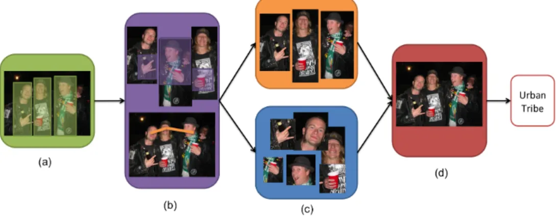
Figure 2.2. Group image categorization. The approach consists of: (a) people detection, (b) local and global descriptor computation, (c) group modeling and (d) classification. . . 6

Figure 2.3. Person part detection examples. . . 8

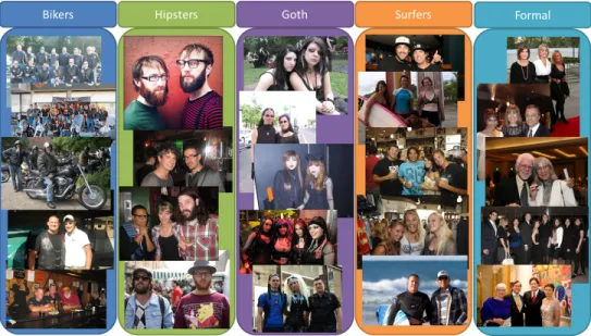
Figure 2.4. Examples of social groups in the Urban Tribes dataset. The images show a wide range of inter-class and intra-class variability. More details can be seen at the dataset website. . . 12

Figure 2.5. Confusion matrix for classification results obtained with (a)BoP_30k and (b) SV M₈, using 80% of the data for training. The rows show results in alphabetical order of the labels (detailed in Table 2.4, from top to bottom. To enhance contrast the color scale is set to[0,0.6]. . . 16

Figure 2.6. Examples of classification results. These images have been classified as

hipstersin all their tests. The two left images are correct, but the label for

the right two images should begoth. . . 16

Figure 3.1. Example questions of the form “Is objectimore similar to jor objectk?”. 21

Figure 3.2. Random triplets have a different distribution than grid triplets. . . 24

Figure 3.3. When the embedding quality is viewed as the number of triplets gathered (top two graphs), it appears that sampling random triplets one at a time yields a better embedding. . . 25

Figure 3.4. Example images from the dataset. The images in the dataset span a wide range of foods and imaging conditions. The dataset as well as the collected triplets will be made available upon publication. . . 27

Figure 3.5. The median time that it takes a human to answer one grid is shown. The time per each task increases with a higher grid size (more time spent looking at the results) and with a higher required number of near answers (which means more clicks per task). Error bars are 25 and 75-percentile. . 28

Figure 3.6. Results of the human experiments on the food dataset. Left graph: Triplet generalization error when viewed with respect to the total number of triplets. Right: The same metric when viewed with respect to the total cost (to the researcher) of constructing each embedding. . . 29

Figure 3.8. The SNaCK embeddings capture human expertise with the help of machine similarity kernels. . . 46

Figure 3.9. Overview of the SNE-and-Crowd-Kernel (“SNaCK”) embedding method. 47

Figure 3.10. A simple MNIST example to illustrate the advantages of SNaCK’s formu-lation. . . 47

Figure 3.11. Experiment overview on CUB-200. See text for details. . . 48

Figure 3.12. Incremental labeling accuracy of several semi-supervised methods. X axis: how many labels are revealed to each algorithm. Y axis: Dataset labeling accuracy. Error bars show standard error of the mean (σ/√n) across five runs. With 14 clusters, chance is≈0.071. See Sec. 3.5.1 for details. . . 48 Figure 3.13. Embedding examples on CUB-200 Woodpeckers and Vireos created with

“SNaCK”. . . 49

Figure 3.14. Classification accuracy of a linear SVM classifier trained on labels discov-ered by different methods. . . 49

Figure 3.15. Example SNaCK embedding on Yummly-10k.. . . 50

Figure 3.16. Experiment Overview for Yummly-10k. See text for details. . . 50

Figure 3.17. Increasing the number of crowdsourced triplet constraints allows all meth-ods to improve the embedding quality. . . 50

Figure 3.18. An example GUI used to interactively explore and refine concept embed-dings. . . 51

Figure 4.1. Overview of detecting the start of actions on mouse behavior videos. . . 70

Figure 4.2. An example screen shot of the web based network output viewer for videos. 71

Figure 4.3. Examples of labeled action starts from THUMOS’14 showing ambiguity in the annotations. . . 72

Figure 4.4. The complete model consists of a fully connected layer, ReLU, Batch Normalization, two Bi-directional LSTM layers, a fully connected layer then a sigmoid activation layer. The LSTMs each have 256 hidden units. . 73

Figure 4.5. Example frames of behaviors the Mouse Reach Dataset. . . 74

Figure 4.7. Distribution of prediction distances from the ground truth location for the Lift behavior . . . 76

Figure 4.8. Distribution of prediction distances from the ground truth location for the Hand-open behavior . . . 77

Figure 4.9. Distribution of prediction distances from the ground truth location for the Grab behavior . . . 78

Figure 4.10. Distribution of prediction distances from the ground truth location for the Supinate behavior . . . 79

Figure 4.11. Distribution of prediction distances from the ground truth location for the At-mouth behavior . . . 80

Figure 4.12. Distribution of prediction distances from the ground truth location for the Chew behavior . . . 81

LIST OF TABLES

Table 2.1. Individual descriptors. They are computed within the bounding box of each part. . . 9

Table 2.2. Low level group descriptors. These are computed over all image pixels and comprise the scene general information, such as lighting and color. . . 9

Table 2.3. High level group descriptors. These represent higher level semantic infor-mation and are based on the distribution and pose of the detected persons in the group. . . 9

Table 2.4. Summary of Urban Tribes dataset. . . 13

Table 2.5. Average accuracy for the recognition of all classes using different approaches. 15

Table 3.1. Results of the actual Mechanical Turk experiments. Workers are asked to choose thek most similar objects from a grid of n images. $1 worth of questions is invested, giving 100 grid selections. Whennand kare large, each answer yields more triplets. . . 30

Table 4.1. Number of labelled frames with the Mouse Reach Dataset. . . 62

Table 4.2. The Mouse Reach Dataset contains a total of 1165 videos of mice perform-ing the reachperform-ing task. . . 62

Table 4.3. F1 scores for each loss, feature type, and behavior. Matching and Wasser-stein losses outperform the per-frame MSE . . . 62

Table 4.4. p-mAP at depthRec=1 shows the performance of the proposed loss functions on THUMOS’14 at different offset thresholds. The *+FWD networks were trained as forward only LSTM’s, whereas the *+BIDIR networks were bi-directional LSTM’s. . . 66

Table 4.5. Average p-mAP at different depths on the THUMOS’14 dataset. . . 67

Table 4.6. For each loss and feature type, the F-score, precision and recall are re-ported. The Matching and Wasserstein Losses have an improved F-score and precision over MSE, implying fewer false positives. . . 68

ACKNOWLEDGEMENTS

Throughout my graduate career, I have been fortunate enough to have constant support

from those around me. I’d like to thank my Ph.D. advisor, David Kriegman, for being a

patient and willing mentor. I am especially grateful for all our meetings regardless of time

zone differences. I also thank Serge Belongie for his guidance and showing me his enthusiasm

towards research. In addition, I thank Serge for allowing me to be a part of his research group,

SE(3), during a complex transition period. I thank Kristin Branson for also providing me with

mentorship and allowing me to finish my graduate research as a part of her lab.

Next, I’d like to thank my many co-authors and colleagues. In particular, Ana Murillo

was my first mentor on my first graduate research project. We spent many strange, but productive,

hours working together while she was in Spain and I in San Diego. To Kimberly Wilber, I will

always cherish our work together and remember your awe-inspiring spirit towards research and

life. Finally, I thank all the members of all the research labs I have been a part of. Although at

times I felt lost and distracted, every lab welcomed me as a part of their own. For Kai, Steve,

and Oscar for being wonderful senior members of the lab when I first started. To Catherine,

Tsung-Yi, and Zak, thanks for being awesome to hang out and discuss research with. To Alice,

Roian, and Nakul, thanks for being patient with me and helping with my move to Virginia. And

to my friends for being there and making the journey more fun.

Finally, thanks to my family. My parents and brother have been, and continue to be,

supportive in all my endeavors. Although I forget to call and keep in touch, they always forgive

and contact me. To my brother, Paul, I thank you for always helping me out whenever you were

able to. I joke about how you changed professions into a computer related field. But in reality, I

couldnt be happier that you found a profession you enjoy and it is a field that we share.

The work proposed in the first chapter was supported by ONR MURI Grant

#N00014-08-1-0638 and by projects DPI2012-31781, DPI2012-32100 and DGA T04-FSE. The work

described in Chapter 2 was partially supported by an NSF Graduate Research Fellowship award

Experiences. We also wish to thank Laurens van der Maaten and Andreas Veit for insightful

discussions.

The work in this dissertation is based on the following publications.

Chapter 2 is based on “From Bikers to Surfers: Visual Recognition of Urban Tribes,” I. S.

Kwak, A. C. Murillo, P. N. Belhumeur, D. Kriegman, and S. Belongie, British Machine Vision

Conference (BMVC) 2013 [KMB+13]. The dissertation author was the primary investigator.

Chapter 3 is based on the following papers: “Cost-effective hits for relative similarity

comparisons.” M. J. Wilber, I. S. Kwak, and Serge J. Belongie, Second AAAI conference on

human computation and crowdsourcing (HCOMP) 2014 [WKB14a]. and “Learning concept

embeddings with combined human-machine expertise,” M. J. Wilber, I. S. Kwak, D. Kriegman,

and S. Belongie, International Conference on Computer Vision (ICCV) 2015 [WKKB15]. The

dissertation author was one of two contributing authors of this paper in both algorithm and

manuscript development.

Chapter 4 is based on “Detecting the Starting Frame of Actions in Video,” I. S. Kwak,

D. Kriegman, K. Branson and is currently being prepared for submission for publication of the

VITA

2005 Bachelor of Science, Carnegie Mellon Universisty

2015 M.S. in Computer Science, University of California, San Diego

2019 Ph.D. in Computer Science, University of California, San Diego

PUBLICATIONS

I. S. Kwak, D. Kriegman, K. Branson, “Detecting the Starting Frame of Actions in Video.”

Under review.

Wilber, M., Kwak, I. S., Kriegman, D., and Belongie, S. “Learning concept embeddings with combined human-machine expertise.” InProceedings of the IEEE International Conference on

Computer Vision. 2015.

Wilber, Michael J., Iljung S. Kwak, and Serge J. Belongie. “Cost-effective hits for relative similarity comparisons.” InSecond AAAI conference on human computation and crowdsourcing. 2014.

Cao, C., Kwak, I. S., Belongie, S., Kriegman, D., and Ai, H. (2014, July). “Adaptive ranking of facial attractiveness.” InIEEE International Conference on Multimedia and Expo (ICME), 2014. E. Christiansen, I. S. Kwak, S. Belongie, and D. Kriegman. “Face box shape and verification.”

InInternational Symposium on Visual Computing (ISVC), 2013.

I. S. Kwak, A. C. Murillo, P. N. Belhumeur, D. Kriegman, and S. Belongie. “From Bikers to Surfers: Visual Recognition of Urban Tribes.” InBritish Machine Vision Conference (BMVC). 2013.

A. C. Murillo, I. S. Kwak, L. Bourdev, D. Kriegman, and S. Belongie. “Urban tribes: Analyzing group photos from a social perspective.” InComputer Vision and Pattern Recognition Workshops

ABSTRACT OF THE DISSERTATION

Towards solving computer vision problems: datasets, labels, algorithms, and applications

by

Iljung Samuel Kwak

Doctor of Philosophy in Computer Science

University of California San Diego, 2019

Professor David Kriegman, Chair

The solution to a supervised computer vision problem consists of an application,

algo-rithm, input data, and a set of human generated labels. Solving these kinds of tasks involves

collecting large quantities of data, collecting appropriate labels, and developing machine vision

algorithms tailored to the application. Progress on these problems has often benefited from

large scale datasets with high fidelity labels. Successful algorithms display a synergy between

application goals and the size and quality of the dataset. This thesis presents work highlighting

the importance of each component of a supervised vision task.

First, the problem of automatically classifying groups of people into social categories

individual and the entire group of individuals are modeled. Since this was a newly introduced

computer vision problem, a dataset for this task was created. On this dataset, the combined

representation of group and individuals outperforms using only the person representations. This

model showed promising results for automatic subculture classification.

Second, the problem of creating perceptual embeddings based on human similarity

judgements is tackled. This work focuses on triplet similarity comparisons of the form “Is object

imore similar to jork?”, which have been useful for computer vision and machine learning

applications. Unfortunately, triplet similarity comparisons, like many human labeling efforts,

can be prohibitively expensive. This work proposes two techniques for dealing with this obstacle.

First, an alternative display for collecting triplets is designed. This display shows a probe image

and a grid of query images, allowing the user to collect multiple triplets simultaneously. The

display is shown to reduce the cost and time of triplet collection. In addition, higher quality

embeddings are created with the improved triplet collection UI. A 10,000-food item dataset

of human taste similarity was created using this UI. Second, “SNaCK,” a low-dimensional

perceptual embedding algorithm that combines human expertise with automatic machine kernels,

is introduced. Both parts are complementary: human insight can capture relationships that are

not apparent from the object’s visual similarity and the machine can help relieve the human from

having to exhaustively specify many constraints.

Finally, the precise localization of key frames of an action is explored. This work focuses

on detecting the exact starting frame of a behavior, an important task for neuroscience research.

To address this problem, a loss designed to penalize extra and missed action start detections

over small misalignments. Recurrent neural networks (RNN) are trained to optimize this loss.

The model is shown to reduce the number of false positives, an important criteria defined by the

neuroscientist. The performance of the model is evaluated on a new dataset, the Mouse Reach

Dataset, a large, annotated video dataset of mice performing a sequence of actions. The dataset

was created for neuroscience research. On this dataset, the proposed model outperforms related

Chapter 1

Introduction

As technology improves, the amount of data that can be created and collected greatly

increases. Because a large portion of this data is in the form of images and videos, computer

vision is uniquely positioned to help catalog and explore this data. Automatic analysis of visual

data provides an opportunity for collaboration with many fields. In addition to improved data

collection, advancements in technology have allowed more powerful algorithms to be created.

Supervised vision has benefited from these changes in technology.

Through social media, personal photo albums are often shared publicly online. Within

these personal albums, a common type of photo is the group photo. Where a group of friends

have their picture taken together in order to remember a shared moment. The work in Chapter

2 focuses on classifying these group photos into social categories. Understanding the social

categories that individuals ascribe to can help automated systems suggest similar interests for

those individuals. This problem is called Urban Tribe classification, and a new dataset for the

task is provided.

As more data is created and collected, it is not always clear what the best annotations

for new datasets are. Some datasets are not categorical by nature and sometimes the goal of

the dataset is to explore and discover categories. For these tasks, triplet comparisons have

been a useful type of label. Unfortunately, large numbers of triplets need to be collected to be

improvements for collecting triplets and their impact is explored. Second, human collected

triplets are augmented with learned representations.

Precisely detecting the start of actions in video has many useful applications. Within

neuroscience research, being able to pinpoint the exact frame a behavior begins can help

researchers correlate visible actions with neural recordings. The work in chapter 4 describes an

algorithm for detecting the start of behaviors and introduce a dataset for action start detection.

This dataset was labeled by experts in neuroscience and is better suited for precise detection

of events than existing action detection datasets. A structured loss for classifying single video

frames as the start of actions was designed. The proposed loss is competitive on the existing

dataset as well as the collected dataset. Accurately detecting action starts will be extremely

useful many vision applications and in particular for neuroscience research.

The supervised vision pipeline involves data, labels, algorithms, and applications. The

work in this thesis explores this pipeline. The work in chapter 2 designed a new dataset for a

new application. Chapter 3 explores improving interactions between researchers and labelers.

Finally, chapter 4 explores the entire pipeline by designing algorithms and constructing a dataset

Chapter 2

Urban Tribe Classification

2.1

Introduction

The popularity of social media has created a massive influx of images. For some social

media platforms, such as Snapchat and Instagram, uploading and sharing images is a core part

of the user’s experience. Facebook alone receives over 300 million photos a day[Arm]. The

abundance of social media presents a compelling opportunity to analyze the social identities of

individuals captured within images. This points to an excellent opportunity for computer vision to

interact with other fields, including marketing strategies and psychological sociology [CBC+10,

JGC+10].

At the time of publication of the original paper described in this chapter, there had been

major strides in image semantic content analysis (in face, object, scene, and clothing recognition),

but algorithms at that time failed to fully capture information from groups of individuals within

images. For example in Fig. 2.1, visual searches of groups of people often provided uninspiring

results. Rather than matching personal style or social identity, the search provided images with

similar global image statistics. The mainstream media had noticed this deficiency in some recent

discussions [Car12] and wondered when vision algorithms will catch up to their expectations.

Since the publication of the original paper, semantic analysis of image content has

improved greatly. In particular, fashion and group photo analysis have become large fields

recommendations from a single article of clothing [MTSVDH15, HWJD17] and retrieval of

clothing similar to a query article of clothing [LLQ+16, HKHL+15]. Similarly, in group photo

analysis, algorithms for detecting familial relationships [DCSH15] or classifying the type of

gathering [SGCC13] have been created. This chapter’s work represents early research in both

group and style analysis.

!"#$%%"&'()$&*+ ,(*"'+$&+#(-".$/0+

!!!"

!!!"

!!!"

!!!"

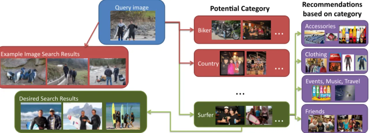
Figure 2.1.The social groups influence the appearance of their members. This work leverages this intuition to classify images of groups of people into social categories. This can improve recommendation systems and user experience with social media, and image search engines can take advantage of this classification and provide more meaningful search results.

In 1985 Michel Maffesoli describedurban tribes[Maf96] as a group of people who have

similar visual appearances, personal style, and ideals. Among tribe members, similar personal

styles often manifest as common accessories such as leather jackets or surfboards. The scene

context also provides useful information: surfers are more likely to be photographed outdoors by

the sea, whereas bikers may congregate at biker bars or be photographed by their bikes on the

road. Though not as discriminative, the overall demeanor between tribes can vary as well, such

as the laid back smiling surfers versus the frowning dark subculture members. The visual cues

shared by members of these tribes provide the basis for this work; members from the same urban

tribe are expected to look more similar than members of different tribes, and they can be easily

identified by people just from visual information.

and applications. More relevant image searches can be conducted; more relevant advertisements

can enhance the web experience of both businesses and consumers; social networks can provide

better recommendations. Urban tribe classification can also improve surveillance of social

demographics. Unfortunately, this categorization problem is difficult because of the ambiguous

nature of social categories and the high intraclass variance. Social categories can evolve and

fracture into separate groups; individuals may exhibit features of multiple urban tribes or certain

individuals may not present a visually salient style at all.

This work highlights the problem of image group categorization from a social perspective,

and contributes towards its solution in several ways. Rather than approaching this problem by

classifying isolated individuals (as most fashion/style analysis works do), this work calculates

meaningful group features and models. Following this idea, a novel recognition pipeline is

presented (see Fig. 2.2) and different modeling approaches are evaluated, following common

frameworks used in other recognition tasks. Finally, a dataset, the Urban Tribes dataset, is

provided. The Urban Tribes dataset has around 100 labeled images per class, from 11

differ-ent classes. This dataset is publicly available in order to facilitate further research on social

categorization of group pictures1.

The work described in this chapter is based on “From Bikers to Surfers: Visual

Recogni-tion of Urban Tribes,” I. S. Kwak, A. C. Murillo, P. N. Belhumeur, D. Kriegman, and S. Belongie,

British Machine Vision Conference (BMVC) 2013 [KMB+13].

2.2

Related Work

The work in this chapter attempts to recognize the content of an image from a social

perspective, which is a growing area of study [VPB09]. Ding and Yilmaz [DY11] show

inter-esting results for the subjective interpretation of action analysis, proposing how to discriminate

positive and negative social relations of individuals in a video sequence. [SWHY11, SLF13]

present promising approaches for predicting the occupation of a subject given that individual’s

Figure 2.2. Group image categorization. The approach consists of: (a) people detection, (b) local and global descriptor computation, (c) group modeling and (d) classification.

clothing and a rough scene context description. Lee and Grauman [LG11b] present a system for

discovering unfamiliar faces in photo albums by leveraging the “social context” of co-occuring

people. Closer to the goals and applications of the work in this chapter, Yu et al.[YJHL11]

analyze a user’s photo album and the associated metadata in order to suggest possible social

groups of interest, e.g., flickr or Facebook groups about flowers or animals. This is closely related

to the goal of analyzing social media, however the approach described in this chapter deals only

with visual information and focuses on the analysis of images with groups of people. Finally,

[WC15] has improved the classification results introduced in this chapter by using powerful

learned feature representations. A common element among most these works is the need for

both global image statistics as well as more semantic individual level attributes.

An important aspect of the work in this chapter involves analyzing a group of individuals

within an image. Group photos have been applied to a wide range of applications since the

publication of the original paper. The group structure or locations of faces has been used to detect

social relationships [SSF17, DCSH15, SGCC13, GC09], such as family members or sports

teammates. Group analysis has also been shown to improve individual identification [MKBK11].

Dhallet al.[DJRG12] highlights the importance of group analysis as a whole, and use it to better

understand the mood of the group of people in an image. In most of these works, the target goal

context.

Automatic fashion analysis has become a well studied topic [KYBB14, HWJD17,

LLQ+16, AHSG17, MTSVDH15, VBK17]. The work in this chapter is most similar to Hipster

Wars [KYBB14], where the authors learn the styles of a variety of social classes. Hipster Wars

focused on images of individuals and explore both discovery and prediction of fashion styles

for social classes. In contrast the work in this chapter focuses on classifying group images

into social categories. In addition to style classification, other researchers have focused on

analyzing the quality of fashion styles [MTSVDH15, AHSG17, HWJD17]. For example, the

authors of [MTSVDH15, HWJD17] can generate outfit recommendations based on an article of

clothing.

Often attributes of individuals are used or predicted by socially motivated vision

algo-rithms. Semantic descriptions of clothing or faces are predicted by many algorithms [AHSG17,

PG11, LLWT15, LLQ+16], and their use has shown to improve many tasks, such as social group

and fashion analysis [SSF17, HWJD17]. In particular, Sunet al.[SSF17] argues for a stronger

connection with social psychology. Semantic attributes help with interpretability and can be

designed with the social domain theory. Hanet al.[HWJD17] also argue for the importance of

attributes for clothing retrieval. Fashion recommendation systems may need to be able to use

either image examples or text based input

The work in this chapter takes advantage of techniques for individual person detection and

description. At the time, one of the leading methods is that of Bourdev and Malik [BM09], which

is based on the detection of person parts namedposelets. Its effectiveness has been demonstrated

for human parsing [WTL11] and recognizing semantic attributes such as hair style or clothing

type [BMM11]. Clothing recognition itself has become a growing field [LSL+12, CGG12]. One

of these works, [YKOB12], mentions the interesting link between visual appearance and social

Person Neck Hat Arm Face Head Torso Eye mouth

Correctly rejected face and person detections

Figure 2.3.Person part detection. Each person hypothesis can have up to six parts and fiducial points for eyes and mouth. The part descriptors are computed within the bounding boxes of these regions. The examples on the left and middle show a close up of the detections. The example on the right presents two face and two person detections that were correctly rejected thanks to the hypothesis construction process proposed (faces must be aligned with a person hypothesis; person bounding box sizes can’t have large deviations).

2.3

Group description

The group modeling involves detecting individuals, extracting individual and group

features and building the group representation, as key steps for the classification detailed later.

2.3.1

Person detection and description

Individuals are detected within the image and each individual is described as a

combi-nation of parts. Similar to [MKB+12], individuals are detected by a combination of poselet

based person detection [BM09] and an open source face detector [ZR12]. A detected person is

composed of six part bounding boxes: face, head, upper head (hat), neck, torso and arms. Both

face and person detections are merged into a single person hypotheses whenever the overlap

of the face and body are above a threshold. This simple step filters out many detected people

that are in the background, rather than the main scene, as shown in the example in Fig. 2.3.

Thus, an image containing ppersons is represented by a set of phypotheses{h₁,h₂, . . . ,h_p}, and each person hypothesis is composed of a set of parts (not all parts need to be detected

to build a hypothesis, as the torso or the arms may not appear in the image). Therefore each

individualh_iis represented by a set with the corresponding parts descriptor vector d_{part name}:

The descriptor set is detailed in Table 2.1, which is computed for each part. This set is

built on the descriptor set used in [MKB+12].

Table 2.1.Individual descriptors. They are computed within the bounding box of each part.

Ratio of skin pixelsvs. total amount of pixels in the patch, obtained with a simple skin-color-based segmentation (normalized to the average face color detected). This descriptor reflects the type of clothing used and how much body is covered with it.

RGB, Luminance and Huehistograms computed for all pixels and computed only for non-skin pixels. This will help modeling the type of clothing used.

Top 3dominant valuesin Red, Green, Blue, Hue and Luminance color bands. Dominant colors in clothes and accessories are very specific at some social categories.

HoG features[DT05], which will help capture the different poses.

2.3.2

Global group descriptors

In order to account for context and group properties, the image is represented by each

of the individualsh_i, as explained above, together with a global group descriptor set,d_global:

G={h1,h2, . . .hp, dglobal}.The global descriptors are split in two sets, low level descriptors

(detailed in Table 2.2) and high level descriptors (detailed in Table 2.3).

Table 2.2.Low level group descriptors. These are computed over all image pixels and comprise the scene general information, such as lighting and color.

Ratioof pixels within the detectedperson bounding boxesvs. total amount of pixels.

RGB, Luminance and Hue histograms computed on all pixels, on pixels out of the detected person bounding boxes, i.e., background pixels.

Gist[OT01] andHOG[DT05] descriptors.

Table 2.3.High level group descriptors. These represent higher level semantic information and are based on the distribution and pose of the detected persons in the group.

Proximitybetween individuals in the image. A histogram of distances between faces are computed and the average ratio of overlap between person bounding boxes.

Alignment orpose of the group. The average angle between a face and its neighboring ones according to a minimum spanning tree computed on the detected faces as proposed in [GC09] is computed.

Scenelayoutof individuals. A histogram of face locations within the image, using a coarse image grid, is computed.

2.4

Group classification

To classify a group of individuals into a social category, the features computed for each

person hypothesis and the group features are modeled jointly. This section describes two different

approaches studied. The group model is built upon the model proposed in past work [MKB+12].

The group is modeled as a set of individuals, combining their responses in a hierarchy of SVM

classifiers. Note that as described, a person hypothesis may have different number of parts

detected, which requires a careful classification framework able to deal with heterogeneous

descriptor sizes.

Bag of Parts-based classification.

Using the Bag of Parts model to represent a group of people, a bag ofmpeople parts

are created and combined with a global descriptor vectord_global. The combined group model will be referred to as G={p1, . . . ,pm,dglobal}. This model combines all visible parts and the

group description. This approach will be named asBoP_k, wherekis the size of the vocabulary used. The vocabulary is built for each part type, by runningk-means clustering for each part.

This vocabulary built for each part type and referred as Vpart ={w1, ...,wk}. wk →histwk =

[countL1, ...,countL j]is the histogram of frequencies for each word in each possible classL.

A signature of the image for each part is created for each vocabularyV_part: hist_part =

[count_w1...count_wk],wherew₁, . . . ,w_k are the words from the correspondingV_part. To be able

to deal with missing parts, each part type is evaluated separately, and later the distances are

combined for each part type intod_BoP(G,L_j). The distance from each part type pdetected in the image to the corresponding class is weighted by its frequency in the training:

dBoP(p,Lj) =1−

∑ki=1(countwi×histwi(j))

k . (2.1)

There are usually several parts of each type in a group image (several faces, arms), and the BoP

models somehow how many occurrences of each possible part (i.e. part word) happen in the

per image. Therefore, the nearest neighbor between each reference,Lj, and test global descriptor

is used:

dglobal(G,Lj) =mintj=1(|gi,gj|), (2.2)

wheret is the number of training images in classLj. This distance is normalized between[0,1]

to allow for easy combination withd_BoP, which is also normalized. Then, withcpossible labels, the label of the group usingBoP_kis calculated as:

L= arg min

j∈[1...c]

(dBoP(G,Lj) +dglobal(G,Lj)). (2.3)

SVM-based classification.

Alternatively, the groupGis represented as a set of persons and the problem is modeled

as finding the most likely classCgiven a particular group imageG, i.e., estimatingP(C|G)for each possible class. In this case, each person hypothesis has a probability for each class and the

final class estimation is a combination of all of them. In this setting, LIBSVM [CL11] is used to

train a multi-class SVM on the person hypotheses and the global descriptors. LIBSVM’s built in

function to calculate probabilities for each class is used. More formally, The goal is to calculate

P(C|G) =P(C|h₁,h₂, . . . ,h_p,d_global),and then the final labelLassigned to the query group as follows:

L= arg max

j∈[1...c]

P(C= j|h1,h2, . . . ,hp,dglobal). (2.4)

P(C|G)is estimated in the following ways:

P(C|G) =P(C|dglobal) p

∏

∏

Figure 2.4. Examples of social groups in the Urban Tribes dataset. The images show a wide range of inter-class and intra-class variability. More details can be seen at the dataset website.

2.5

Experiments and Results

This section evaluates the performance of the proposed algorithms.

2.5.1

Urban Tribes dataset

Creating the Urban Tribe Dataset posed an interesting challenge. Similar to computer

vision problems, such as clothing or beauty evaluation, urban tribe categories can be ambiguous

and subjective. This is a contrast to other classification problems involving people, where

accurate descriptions of each class and its standard appearance can be found, such as age, gender

or occupation evaluation. In order to obtain an unbiased dataset, the classes labels are provided

by Wikipedia. Eight categories from their list of subcultures2to facilitate image collection were

selected. In addition to these social groups, three other classes corresponding to typical social

venues (formal events, dance clubs and casual pubs) were added. These classes are intended to

include some of the most common social event pictures that may not belong to a clear subculture,

but still present common appearances in clothing style.

Table 2.4.Summary of Urban Tribes dataset.

Label # images # people Label # images # people Label # images # people

biker 114 443 hip-hop 90 253 club 100 365

country 107 347 hipster 102 288 formal 103 414

goth 99 226 raver 116 305 casual/pub 125 459

heavy-metal 102 266 surfer 100 333

For each of the selected classes, images of groups of people were searched with different

search engines. Group labels were used as search keywords combined with location and event

keywords such asbar,venue,cluborconcert. Example search terms include ’bikers’ and ’biker

bar’. The dataset contains a broad range of scenarios for each class, both indoor and outdoor

venues, large group pictures acquired from the distance and close-up images, etc. As shown in

Fig. 2.4, the groups show a variety of realistic conditions and most classes present high intra-class

variation in appearance. Table 2.4 shows the class labels as well as the number of images (#

images) per class and total amount of detected persons for each class (# people). Although

the number of images per class was balanced, the number of detected persons per image was

different depending on the group.

2.5.2

Social group recognition experiments

This section evaluates the performance of the proposed algorithms and the most promising

paths towards this novel problem framework. Training and testing images were randomly selected

from each of the categories for 50 different iterations. Note that for the 11 classes in the Urban

Tribes Dataset, chance classification is ₁₁1 =0.09. For each experiment, a fixed number of the

images from each class are used for learning the models, and the rest of images are used for

testing. A test is considered correct if the most likely group label is correct according to the

ground truth labels.

As explained in section 2.4, the Bag of Parts modeling builds a visual vocabulary for each

part using the training set, withkvisual words per vocabulary. After evaluating different values

when increasingkuntilk=30. The other approach modeled the group as a set of people and used

the training set descriptors to train several SVM classifiers. Different options were evaluted: 1)

SV M₁, training a single SVM with all the descriptors of each person concatenated, including null

values for non-detected parts and replicating the same global descriptor for all hypothesis from a

particular image; 2)SV M₂, training one SVM for all part descriptors similarly concatenated and

a second SVM for the global image descriptors; 3)SV M₈, training a separated SVM classifier for

each part descriptor set and an additional SVM for the global image descriptors. The responses

from all the SVMs in each case are simply combined, providing a final probability of each image

being of a particular class. The optionSV M1provided significantly lower performance than the

rest during the preliminary tests, therefore results for configuration are not provided for the rest

of experiments.

Results from [WC15] are also provided, which were computed after the publication

of the original paper. [WC15] create a model called NetSDense, which uses features from an

AlexNet [KSH12] network pre-trained on ImageNet [RDS+14]. NetSDense consists of two

AlexNets. One for person crop classification and the other for scene image classification. A

person and scene SVM classifier uses the feature representations from AlexNet to compute

probabilities for an input to belong to a class. The person class probabilities are averaged and

weighted by the scene class probability.

Table 2.5 shows a summary of recognition experiments with different amount of training

data and different amount of parts used in the modeling, given the most suitable configurations

found for each modeling option considered (BoP_30k, SV M₂ and SV M₈). Column allParts+

global shows the accuracy when combining all person parts and global descriptors;allParts

shows the accuracy when combining only person parts;global(scene)column shows the results

if only the global descriptors are used).

The last columns show additional baseline results:individualshows the average accuracy

when each person is classified independently from the rest of the group, i.e., there is no consensus

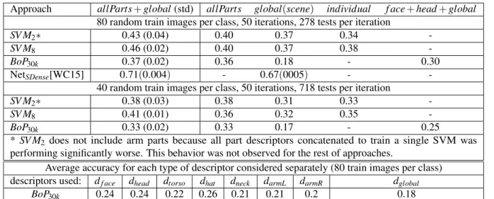
Table 2.5.Average accuracy for the recognition of all classes using different approaches.

Approach allParts+global(std) allParts global(scene) individual f ace+head+global

80 random train images per class, 50 iterations, 278 tests per iteration

SV M2∗ 0.43 (0.04) 0.40 0.37 0.34

-SV M8 0.46 (0.02) 0.40 0.37 0.38

-BoP30k 0.37 (0.02) 0.36 0.18 - 0.30

NetSDense[WC15] 0.71(0.004) - 0.67(0005) - -40 random train images per class, 50 iterations, 718 tests per iteration

SV M2∗ 0.38 (0.03) 0.38 0.31 0.33

-SV M8 0.41 (0.01) 0.36 0.32 0.35

-BoP30k 0.33 (0.02) 0.33 0.17 - 0.25

*SV M2 does not include arm parts because all part descriptors concatenated to train a single SVM was

performing significantly worse. This behavior was not observed for the rest of approaches.

Average accuracy for each type of descriptor considered separately (80 train images per class) descriptors used: df ace dhead dtorso dhat dneck darmL darmR dglobal

BoP30k 0.24 0.24 0.22 0.26 0.21 0.21 0.2 0.18

using the Bag of Parts configuration used in the referred previous work [MKB+12]. The last

rows in the table show the contribution of each type of descriptor separately. This analysis is

shown for the BoP approach, since it provides the classification result per part. For all modeling

options, even just one set of descriptors was able to classify the images above chance, but the

final classification scores are clearly improved when all the parts from all the individuals in

the image are combined. Particularly interesting is the increase due to the use of global group

information. Additionally, we have noted that the global descriptors classifier would correctly

predict the correct label between 10% to 15% of the tests (depending on the modeling option).

This supports the idea that group and context provide complementary information to person local

parts.

Among the models described in 2.4, the SVM based classification provided the best

results at the time. It is probably better at learning which components of each descriptor set

are more discriminative. We experimented with a reduced set of attributes for BoP approaches

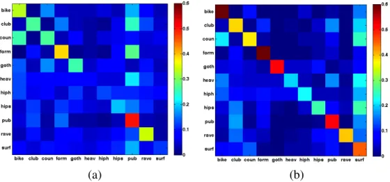
did not improve the performance. From the confusion matrices shown in Fig. 2.5, interesting

hints for future improvements can be seen, such as the clear confusion in both matrices between

(a) (b)

Figure 2.5.Confusion matrix for classification results obtained with (a)BoP_30kand (b)SV M₈, using 80% of the data for training. The rows show results in alphabetical order of the labels (detailed in Table 2.4, from top to bottom. To enhance contrast the color scale is set to[0,0.6].

Figure 2.6.Examples of classification results. These images have been classified ashipstersin all their tests. The two left images are correct, but the label for the right two images should be

goth.

descriptors or attributes. Analyzing the results, all images have been included, in average, in the

test set of 12 experiments. Figure 2.6 shows some sample classification results.

The NetSDensemodel, benefiting from powerful learned representations, out performs all

results by a significant margin. The authors of [WC15] also report classification results on just

each person, 0.47 and all the people, 0.67 in a scene. These results aren’t included in Table 2.5

because the human crops are not from poselets. Interestingly, these results match the findings

2.6

Conclusions and Future Work

An individual’s social identity can be defined by the individual’s association with various

social groups. Often these social groups influence the individual’s visual appearance. An

exhaustive baseline analysis is provided for the task as well as a dataset to aid future research.

The task introduced in this work opens opportunities for computer vision to improve targeted

advertising and social monitoring and provide more tailored experiences with social media.

The work in this chapter has shown that group representations are powerful. Although

more recent learned representations have outperformed past results, the recent results do not

fully capture the group structure of the individuals in an image. Future work should learn

group structure features. For example, Graph Neural Networks [ZCZ+18] could be used to

learn a representation for the group. With a graph neural network, detected individuals could

be represented by nodes in a graph and the network could model the structure as a whole.

Alternatively, the Transformer architecture [VSP+17] has shown promising results in natural

language parsing and could also be used to model the group structure. Here the representation

of individuals could be passed in as a sequence. In either case the entire group is an input to a

network architecture in order to learn group features.

2.7

Acknowledgments

Chapter 2 is based on “From Bikers to Surfers: Visual Recognition of Urban Tribes,” I. S.

Kwak, A. C. Murillo, P. N. Belhumeur, D. Kriegman, and S. Belongie, British Machine Vision

Chapter 3

Collecting & Using Human Judgements of

Similarity

3.1

Introduction

Rankings and similarity constraints provided by humans have been used in many fields,

such as psychometrics, social sciences, and computer vision. A common application for these

con-straints is to construct embeddings for visualization and exploration. The overall goal of the work

in described in this chapter is to generate these perceptual embeddings. Many researchers use

similar embeddings to enhance the performance of classifiers [SKP15, BHW+14, WHB+14a],

build retrieval systems [VdMW12b, McF12], and create visualizations that help experts better

understand high-dimensional spaces [DBH14, DSK+14]. This problem is tackled by improving

the collection of similarity constraints and by combining human similarity constraints with

learned representations.

The work in this chapter focuses on collecting and using the triplet constraint. Triplet

constraints are of the form, “Is objectimore similar to object jor objectk?”. These constraints

have been used in many vision applications, such as face recognition [SKP15] and image

retrieval [FSSM07]. Additionally triplets have been shown to be a more reliable form of human

similarity constraint [Ken48] than human based rankings or human pairwise similarity constraints.

By combining learned representations and human generated triplets, perceptual embeddings can

Unfortunately, asking experts to exhaustively and authoritatively annotate a dataset

is not always possible [BEK+12]. Additionally, triplet based comparisons can potentially

have O(n3) complexity [TLB+11]. Hiring actual domain experts is often out of the question,

and even crowdsourcing websites such as Mechanical Turk can be prohibitively expensive.

Intelligently sampling comparisons can help alleviate this issue [TLB+11, JN11], but the number

of constraints to collect can still be too large for human annotation. To reduce the cost of

collecting triplets, a new user interface and query was designed and evaluated.

This chapter describes methods for improving the creation of perceptual embeddings

from triplet constraints. In 3.3, UI guidelines for collecting similarity comparisons are described,

with insights on how to manage the trade-off between user burden, embedding quality, and cost.

The method’s effectiveness is shown on a series of synthetic and human-powered experiments. In

3.4, an algorithm for creating perceptual embeddings called SNE-and-Crowd-Kernel Embedding,

SNaCK, is presented. The algorithm combines expert triplet hints with machine assistance to

efficiently generate concept embeddings. The effectiveness of SNaCK embeddings are shown on

tasks such as visualization, concept labeling, and perceptual organization.

The SNaCK algorithm performs dimensionality reduction in order to create visualizations.

ConsiderNobjects,X={xi}_iN₌₁andxi∈RD. The goal of dimensionality reduction is to produce

a targetd-dimensional embeddingY ={y_i}N

i=1,yi∈Rd, whered<D. A classic technique for

creating low dimensional visualization is metric Multidimensional Scaling (MDS) [Wic03,

KW78]. MDS creates the embedding,Y, by attempting to preserve distances between points in

the original space by optimizing:

min

Y

∑

i6=j=0,1,...,N

(de(xi,xj)−de(yi,yj))2 (3.1)

whered_eis the Euclidean distance. Isomap [BS02] extends MDS by replacingd_e(x_i,x_j)

withd_g(x_i,x_j), whered_g is the geodesic distance between points. This change helps Isomap to preserve local structure in the lower dimensional representation. t-Distributed Stochastic

Neighbor Embedding (t-STE) [VdMH08], which will be described in detail in Section 3.4.1, also

follows the intuition of MDS, but instead converts distances to conditional probabilities. t-STE

attempts to match the probability distribution of the original and target spaces. The probability

represents the likelihood that a point chooses another as its neighbor. Like Isomap, this helps

t-SNE preserve the local structure in the embedding. An alternative to metric MDS is non-metric

MDS (NMDS) [Kru64]. Non-metric MDS optimizes an alternative cost:

min

Y

∑i6=j=0,1,...,N(dr(xi,xj)−de(yi,yj))2

∑i6=j=0,1,...,Nde(yi,yj)

(3.2)

wheredr is any monotonic function, but it typically computes the rank order of

pair-wise distances. This formulation is interesting because it no longer requires knowing the exact

distances between points in the original space, which is useful when requesting similarities from

humans. Rather than requiring the full rank ordering of points, generalized non-metric MDS

(GNMDS) [AWC+07] focuses on pairwise comparisons of similaritiesd_e(x_i,x_j)2<d_e(x_k,x_l)2. When collecting data from humans, this formulation is even more appealing than NMDS and

MDS. Stochastic Triplet Embedding (t-STE) [VdMW12b], described in detail in Section 3.4.1, is

another algorithm for embedding points using relative comparisons. t-STE converts the pairwise

comparisons into probabilities and creates an embedding that matches the probability distribution

of the original space. The SNaCK algorithm proposed in this chapter combines t-SNE and t-STE.

The work described in this chapter based on the following papers: “Cost-effective hits

for relative similarity comparisons.” M. J. Wilber, I. S. Kwak, and Serge J. Belongie, Second

AAAI conference on human computation and crowdsourcing (HCOMP) 2014 [WKB14a]. and

“Learning concept embeddings with combined human-machine expertise,” M. J. Wilber, I. S.

Kwak, D. Kriegman, and S. Belongie, International Conference on Computer Vision (ICCV)

Figure 3.1. Questions of the form “Is objectimore similar to jor objectk?” have been shown to be a useful way of collecting similarity comparisons from crowd workers. Traditionally these comparisons, or triplets, would be collected with a UI shown at the top. Here, triplets are collected using a grid of images and ask the user to select the two most similar tasting foods.

3.2

Related Work

Perceptual embeddings have been used for a wide range of applications. In [AWC+07],

the authors created a two-dimensional embedding where one axis represented the brightness

of an object, and the other axis represented the glossiness of an object. [vdMW12a, McF12]

construct an embedding based on musical artist similarity. The goal is to use triplets to collect

and construct perceptual similarity embeddings. And as mentioned before, SNaCK combines

aspects of both t-Distributed Stochastic Neighbor Embedding (t-SNE, from [VdMH08]) and

Stochastic Triplet Embedding (t-STE, from [VdMW12b]).

The work in this chapter focuses on using triplet similarity constraints. In addition to

being useful for constructing perceptual embeddings [vdMW12a, FG09, GWKP11, McF12],

triplets have been used for classification tasks as well. In this case, triplets can be automatically

generated using categorical labels, where “objectiis more similar to object jthan objectk”, ifi

and jare in the same class andiandkare not in the same class. [SKP15] showed state of the art

face recognition results and [HBL17, CGZ+16] has shown that the re-identification problem can

also take advantage of triplet similarity constraints.

Alternative similarity constraints such as pairwise or rank ordering have also been used

to create perceptual embeddings. However when collecting these constraints from humans, it has

been shown that triplet constraints have been most consistent [Mil56, Ken48, DBH14]. In an

experiment comparing the speed and effectiveness of pairwise, triplet, and spatial arrangement

embeddings, [DBH14] found that triplet comparisons yield the least variance of human perceptual

similarity judgments than other methods. Unfortunately, triplet embeddings can requireO(n3)

constraints to be uniquely specified [KvL14], even though many triplets are strongly correlated

and do not contribute much to the overall structure [SKP15].

A variety of methods have focused on reducing the number of triplets to collect [TLB+11,

JN11]. These algorithms focus on collecting triplets one at a time, but sampling the best triplets

captured with a very small number of triplets, since most triplets convey redundant information.

For instance, Crowd Kernel Learning [TLB+11] considers each triplet individually, modeling the

information gain learned from that triplet as a probability distribution over embedding space. This

chapter includes a new UI design to improve the speed of triplet collection and leverages learned

representations to reduce the number of triplets required. Since the publication of the UI design,

a few works [LHLF15, PMB18] have used the proposed design for collecting triplets. Others

have altered the initial design to collect alternative types of similarity constraints [VMN+16].

3.3

Cost Effective Hits

Instead of asking “Is objectimore similar to object jor objectk?”, humans are presented

with a probe image and ask “Markkimages that are most similar to the probe,” as in Fig. 3.1.

This way, with a grid of sizen, a human can generatek·(n−k)triplets per task unit. This kind of query allows researchers to collect more triplets with a single screen. It allows crowd workers

to avoid having to wait for multiple screens to load, especially in cases where one or more of the

images in the queried triplets do not change. This also allows crowd workers to benefit from the

parallelism in the low-level human visual system [Wol94]. Because collecting triplets require

human effort, the right way to measure the embedding quality is with respect to human cost

rather than the number of triplets. This human cost is related to the time it takes crowd workers

to complete a task and the pay rate of a completed task. Some authors [WHB+14b, TLB+11]

already incorporate these ideas into their work but do not quantify the improvement. The goal is

to formalize their intuitive notions into hard guidelines.

It is important to note that the distribution of grid triplets is not uniformly random, even

when the grid entries are selected randomly and provided perfect answers. No authors that use

grids acknowledge this potential bias even though it deteriorates quality of the collection of

triplets, as will be shown in the experiments. Figure 3.2 shows a histogram of how many times

0 1 2 3 45 6

7

How often do objects appear in triplet results? (Grid 16 choose 4)

12000 1400 1600 1800 2000 2200 2400 5 10 15 20 25 30

(Random sampling)

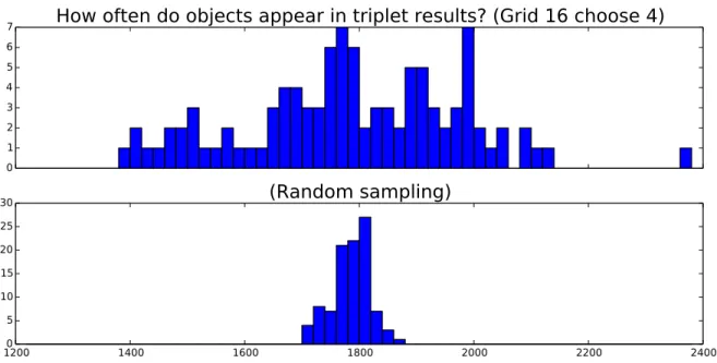
Figure 3.2. Random triplets have a different distribution than grid triplets. The top histogram shows the occurrences of each object within human answers for “Grid 16 choose 4” triplets, the bottom is a histogram of sampling random triplets individually. The variation when using grid triplets (top) is much wider than the variation when sampling triplets uniformly.

object occurs in the answers about ˆµ =1785 times, but the variation when using grid triplets,

top histogram, is much wider ( ˆσ ≈187.0) than the variation when sampling triplets uniformly (bottom histogram, ˆσ =35.5). This effect is not recognized in the literature by authors who use

grids to collect triplets. When using grid sampling, some objects can occur far more often than

others, suggesting that the quality of certain objects’ placement within the recovered embedding

may be better than others. The effect is less pronounced in random triplets, where objects appear

with roughly equal frequency. This observation is important to keep in mind because the unequal

distribution influences the result.

3.3.1

Synthetic Experiments

The goal of the synthetic experiments is to answer two questions: Are the triplets acquired

from a grid of lower quality than triplets acquired one by one? Second, even if grid triplets are

lower quality, does their quantity outweigh that effect? To find out, synthetic “Mechanical

103 ₁₀4 ₁₀5 ₁₀6 ₁₀7 Number of triplets 0.40 0.45 0.50 0.55 0.60 0.65 0.70 0.75 0.80 Generalization Error Leave-1-out NN error Grid 12, choose 3 Grid 12, choose 4 Grid 12, choose 5 Grid 12, choose 6 Random triplets 103 ₁₀4 ₁₀5 ₁₀6 ₁₀7 Number of triplets 0.15 0.20 0.25 0.30 0.35 0.40 0.45 0.50 Generalization Error Constraint Error Grid 12, choose 3 Grid 12, choose 4 Grid 12, choose 5 Grid 12, choose 6 Random triplets 0 1000 2000 3000 4000 5000 6000 7000 8000 9000 Number of screens 0.40 0.45 0.50 0.55 0.60 0.65 0.70 0.75 0.80 Generalization Error Leave-1-out NN error Grid 12, choose 3 Grid 12, choose 4 Grid 12, choose 5 Grid 12, choose 6 Random triplets 0 1000 2000 3000 4000 5000 6000 7000 8000 9000 Number of screens 0.15 0.20 0.25 0.30 0.35 0.40 0.45 0.50 Generalization Error Constraint Error Grid 12, choose 3 Grid 12, choose 4 Grid 12, choose 5 Grid 12, choose 6 Random triplets

Music dataset, 20 dimensions

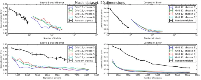
Figure 3.3. When the embedding quality is viewed as the number of triplets gathered (top two graphs), it appears that sampling random triplets one at a time yields a better embedding. However, when viewed as a function of human effort, grid triplets create embeddings that converge much faster than individually sampled triplets. See text for details.

objects are shown. The synthetic workers use Euclidean distance within a groundtruth embedding

to choosekgrid choices that are most similar to the probe. As a baseline, triplet comparisons

are randomly sampled from the groundtruth embedding using the same Euclidean distance

metric. After collecting the test triplets, a query embedding is built with t-STE [VdMW12b] and

compared to the groundtruth. This way, the quality of the embedding with respect to the total

amount of human effort is measured, which is the number of worker tasks. This is not a perfect

proxy for human behavior, but it does let us validate the approach, and should be considered in

conjunction with the actual human experiments that are described later.

Dataset. UI paradigm is evaluated on the music similarity dataset from [VdMW12b].

The dataset contains 9,107 human-supplied triplets for 412 artists.

Metrics. The quality of the embedding is evaluated using two metrics from [vdMW12a]:

Triplet Generalization Error, which counts the fraction of the groundtruth embedding’s triplet

constraints that are violated by the recovered embedding; and Leave-One-Out Nearest Neighbor

error, which measures the percentage of points that share a category label with their closest

different things: Triplet Generalization Error measures the triplet generator UI’s ability to

generalize to unseen constraints, while NN Leave-One-Out error reveals how well the embedding

models the (hidden) human perceptual similarity distance function. These metrics test the impact

that different UIs have on embedding quality.

Results. The experiments show that even though triplets acquired via the grid converge

faster than random triplets, each individual grid triplet is of lower quality than an individual

random triplet. Figure 3.3 shows how the music dataset embedding quality converges with

respect to the number of triplets. If triplets are sampled one at a time (top two graphs), random

triplets converge much faster on both quality metrics than triplets acquired via grid questions.

However, this metric does not reveal the full story because grid triplets can acquire several triplets

at once. When viewed with respect to the number of screens (human task units), as in the bottom

two graphs in Figure 3.3, the grid triplets can converge far faster than random with respect to the

total amount of human work. This implies that “quality of the embedding wrt. number of triplets”

can be the wrong metric to optimize. A researcher who only considers the inferior performance

of grid triplets on the per-triplet metric will prefer sampling triplets individually, but they could

achieve much better accuracy using grid sampling even in spite of the reduced quality of each

individual triplet. In other words, efficient collection UIs are better than random sampling, even

though each triplet gathered using such UIs does not contain as much information.

3.3.2

Human Experiments

To verify that the UI modifications build better embeddings, Mechanical Turk experiments

were run on a set of 100 food images sourced from Yummly1recipes with no groundtruth. The

images were filtered so that each image contained roughly one entr´ee. For example, images

of sandwiches with soups were avoided. Example images are shown in Fig. 3.4. For each

experiment, the same amount of money was allocated for each hit, allowing the embedding quality

with respect to cost to be quantified. This dataset and the human annotations are available for

Figure 3.4. Example images from the dataset. The images in the dataset span a wide range of foods and imaging conditions. The dataset as well as the collected triplets will be made available upon publication.

download at the companion website, https://vision.cornell.edu/se3/projects/cost-effective-hits/.

Design. For each task, a random probe and a grid ofnrandom foods are shown. The

user is asked to select thek objects that “taste most similar” to the probe. nis varied across

(4,8,12,16)andkis varied across(1,2,4). Three independent repetitions of each experiment

were run. Each HIT paid $0.10, which includes 8 usable grid screens and 2 catch trials. To

evaluate the quality of the embedding returned by each grid size, the same “Triplet Generalization

Error” was used as in the synthetic experiments: all triplets from all grid sizes are gathered

and a reference embedding via t-STE is constructed. Then, to evaluate a set of triplets, a target

embedding is constructed, and the number of reference embedding’s constraints violated by the

target embedding are counted. Varying the number of HITs shows how fast the embedding’s

4

8

12

16

Grid size

0

2

4

6

8

10

12

14

Seconds

Timing tasks

Choose 4

Choose 2

Choose 1

Figure 3.5. The median time that it takes a human to answer one grid is shown. The time per each task increases with a higher grid size (more time spent looking at the results) and with a higher required number of near answers (which means more clicks per task). Error bars are 25 and 75-percentile.

102 ₁₀3 ₁₀4 Number of triplets 0.1 0.2 0.3 0.4 0.5 Generalization Error Grid 4 choose 2 Grid 8 choose 4 Grid 12 choose 4 Grid 16 choose 4 Random triplets CKL $0.00 $1.00 $2.00 $3.00 $4.00 $5.00 Total cost ($) 0.1 0.2 0.3 0.4 0.5 Generalization Error Grid 4 choose 2 Grid 8 choose 4 Grid 12 choose 4 Grid 16 choose 4 Random triplets CKL

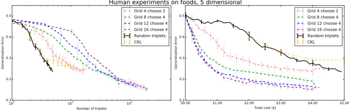
Human experiments on foods, 5 dimensional

Figure 3.6. Results of the human experiments on the food dataset. Left graph: Triplet generalization error when viewed with respect to the total number of triplets. Right: The same metric when viewed with respect to the total cost (to the researcher) of constructing each embedding.

Baseline. Since the goal is to show that grid triplets produce better-quality embeddings

at the same cost as random triplets, random(i,j,k)constraints are collected from crowd workers

for comparison. Unfortunately, collecting all comparisons one at a time is infeasible (see the

“Cost” results below), so instead, a groundtruth embedding from all grid triplets is construct and

random constraints are uniformly sampled from the embedding. This is unlikely to lead to much

bias because 39% of the possible unique triplets were collected, meaning that t-STE only has to

generalize to constraints that are likely to be redundant. All evaluations are performed relative to

this reference embedding.

3.3.3

Results

Two example embeddings are shown in Fig. 3.7.

Cost. Across all experiments, 14,088 grids are collected, yielding 189,519 unique triplets.

Collecting this data cost $158.30, but sampling this many random triplets one at a time would

have cost $2,627.63, which was far outside this project’s budget2. If the 16-choose-4 grid strategy

is used (which yields 48 triplets per grid), then all unique triplets would be able to be sampled

2_{There are 100·99·98/2=485,100 possible unique triplets and each triplet answer would cost one cent.}