Targeted Maximum Likelihood Estimation for Dynamic Treatment Regimes in Sequential Randomized Controlled Trials

University of California, Berkeley

U.C. Berkeley Division of Biostatistics Working Paper Series

Year  Paper

Targeted Maximum Likelihood Estimation for

Dynamic Treatment Regimes in Sequential

Randomized Controlled Trials

Paul Chaffee

Mark J. van der Laan

∗_{University of California, Berkeley, Division of Biostatistics, [email protected]} †_{University of California, Berkeley, Division of Biostatistics, [email protected]}

This working paper is hosted by The Berkeley Electronic Press (bepress) and may not be commer-cially reproduced without the permission of the copyright holder.

http://biostats.bepress.com/ucbbiostat/paper277 Copyright c2011 by the authors.

Targeted Maximum Likelihood Estimation for

Dynamic Treatment Regimes in Sequential

Randomized Controlled Trials

Abstract

Sequential Randomized Controlled Trials (SRCTs) are rapidly becoming essential tools in the search for optimized treatment regimes in ongoing treatment settings. Analyzing data for multiple time-point treatments with a view toward optimal treatment regimes is of interest in many types of afflictions: HIV infection, Atten-tion Deficit Hyperactivity Disorder in children, leukemia, prostate cancer, renal failure, and many others. Methods for analyzing data from SRCTs exist but they are either inefficient or suffer from the drawbacks of estimating equation method-ology. We describe an estimation procedure, targeted maximum likelihood esti-mation (TMLE), which has been fully developed and implemented in point treat-ment settings, including time to event outcomes, binary outcomes and continuous outcomes. Here we develop and implement TMLE in the SRCT setting. As in the former settings, the TMLE procedure is targeted toward a pre-specified pa-rameter of the distribution of the observed data, and thereby achieves important bias reduction in estimation of that parameter. As with the so-called Augmented Inverse Probability of Censoring Weight (A-IPCW) estimator, TMLE is double-robust and locally efficient. We report simulation results corresponding to two data-generating distributions from a longitudinal data structure.

1

Introduction

1.1

Background

The treatment of many types of afflictions involves ongoing therapy—that is, application of therapy at more than one point in time. Therapy in this con-text often involves treatment of patients with drugs, but need not be limited to drugs. For example, the use of pill organization devices (“pillboxes”) has been studied as a means to improve drug adherence (Petersen et al., 2007), and others (Moodie et al., 2009) have studied the optimum time at which infants should stop breastfeeding.

A common setting for ongoing treatment therapy involves randomization to initial treatment (or randomization to initial treatment within subgroups of the population of interest), followed by later treatments which may also be randomized, or randomized to a certain subset of possible treatments given that certain intermediate outcomes occurred, by definition, after the initial treatment. Examples from the literature include treatment by antipsychotic medications for reduction in severity of schizophrenia symptoms (Tunis et al., 2006), treatment of prostate cancer by a sequence of drugs determined by success or failure of first-line treatment (Bembom and van der Laan, 2007), when HIV patients should switch treatments (Orellana et al. 2010, van der Laan and Petersen 2007) and many others.

Suppose, for example, that every subject in a prostate cancer study is ran-domized to an initial pair of treatments (A or B, say), and if a subject’s tumor size increases or does not decrease, the subject is again randomized to A or B at the second treatment point. On the other hand, if the subject does well on the first treatment (tumor size decreases, say), then he or she is assigned the same treatment at the second time point as the first. The general term for multiple time point treatments in which treatments after the first-line are assigned in response to intermediate outcomes is dynamic treatment regimes or dynamic treatment rules (Murphy et al., 2001). If the intermediate outcome in such SRCTs is affected by initial treatment, and in turn affects decisions at the second time-point treatment as well as the final outcome, then it is a so-called “time-dependent confounder.”

1.2

Existing Procedures

A number of methods have been proposed to estimate parameters associ-ated with such a study. This article describes implementation of targeted maximum likelihood estimation for two time-point longitudinal data struc-tures, and is based on the framework developed for general longitudinal data structures presented in van der Laan (2010a,b).

Tunis et al. (2006) use inverse probability of treatment weighted (IPTW) methods, Marginal Structural Models and the so-called “g-estimation” method for analyzing the causal effect of a “continuous” treatment regime of atypi-cal antipsychotic medications on severity of schizophrenia symptoms. This study/analysis involved no time-dependent confounders, however. Orellana et al. (2010) use structural marginal mean models, IPTW and the so-called augmented inverse probability of censoring weight (A-IPCW) estimators with a view toward estimating optimal treatment regimes for switching to HAART therapy among HIV-positive patients. Laber et al. (2009) use Q-learning to estimate optimal dynamic treatment regimes in Attention Deficit Hyperac-tivity Disorder in children. Guo and Tsiatis (2005) develop what they call a “Weighted Risk Set Estimator” for use in two-stage trials where the outcome is a time-to-event (such as death). Bembom and van der Laan (2007) ap-ply simple g-computation and IPTW estimation procedures in analyzing the optimum response of prostate cancer patients to randomized first-line treat-ment followed by second-line treattreat-ment which was either 1) the same as the first line treatment if that had been deemed successful, or 2) randomized to three remaining treatments if the first line had failed. This type of trial and data closely resembles the data we simulate and analyze in the present study, though we add baseline covariates and more than 2 levels of success in the intermediate biomarker covariate in order to generalize the data structure to more types of scenarios.

We present a new estimator for this longitudinal data structure: the tar-geted maximum likelihood estimator (van der Laan et al., 2009). TMLE has application in a wide range of data structures and sampling designs. Though this estimator can be applied to a broad range of data structures of longitudinal type, we focus here on the estimation of treatment-rule-specific mean outcomes. This also covers static treatment regimes for the given data structures.

the scenarios we intend to analyze. Once we have specified a counterfactual target parameter of interest and equated it with a well-defined mapping from conditional distributions of the data to a real number, we describe TMLE in broad outline, and in particular, the implementation of two different es-timators grounded in the general TMLE approach. Specifically we present the so-called efficient influence curve for certain parameters of interest and show the relationship between elements of this object and elements of the targeted maximum likelihood estimators. Following these general descrip-tions we present simulation results, including details of specific treatment rules, data generation and results in terms of bias, variance and relative mean squared error. A short discussion of the results follows.

2

Data Structure and Likelihood

In the settings of interest here, a randomly sampled subject has data struc-ture O = (L(0), A(0), L(1), A(1), Y = L(2)) ∼ P0, where L(0) indicates a

vector of baseline covariates, A(0) is initial randomized treatment, L(1) is, say, an intermediate biomarker (which we first consider as binary), A(1) is the second time point treatment (which we also take as binary), Y = L(2) is the clinical outcome of interest and P0 is the joint distribution of O. We

take the data to be n i.i.d. copies of O. We also assume A(1) can be set in response to L(1). The patient’s full treatment is therefore (A(0), A(1)), and specific realizations of (A(0), A(1)) may or may not constitute realizations of a specific dynamic treatment rule. Such “rules” are dynamic in the sense that the regimen can be set according to a patient’s response to treatment over time. However, even ifA(0) andA(1) are both unconditionally random-ized, parameters of the distribution of the above data can nevertheless be identified which correspond with dynamic treatment regimens.

The data structure for such an experimental unit can be thought of as a time series in discrete time. For many of the (not necessarily regularly-spaced) time points there may be no observation of interest, and at others measur-able events of interest occur. Many measurmeasur-able events may occur at the same time—e.g., assignment of treatment and recording of measured characteris-tics. A specified set of all measured variables that respects this time-ordering, together with possible additional knowledge about the ordering and relation-ships of the variables, implies a particular statistical graph. The graph is a representation of each variable and its causal relation to its parent nodes,

the latter being defined as all variables that preceded it in the specified time-ordering and are either direct or indirect causal antecedents. The graph can be modified to encode not only the time-ordering of the variables but also possible additional causal assumptions. The likelihood of this unit-specific data structure can be factorized according to the specified time-ordering, where the factors consist of the conditional distribution of each node given its parents, for all nodes in the graph.

The likelihood of the data described above can be factorized as

p(O) = 2 Y j=0 P[L(j)|L¯(j−1),A¯(j−1)] 1 Y j=0 P[A(j)|L¯(j),A¯(j−1)], (1)

where ¯A(j) = (A(0), A(1), ..., A(j)) and ¯L(j) is similarly defined. Factorizing the likelihood in this way is suggested by the time–ordering of the variables in O. That is, we assume L(0) is followed by A(0), and then L(1), A(1) and outcome L(2) occur in that order. The above formula is the most general in the sense that each factor is represented as a function of its parents as defined by the time-ordering of the data, but in some cases a particular factor may be a function of fewer nodes than this representation suggests. (An example is given later in this section.)

Equation (1) is an example of the general longitudinal factorization

p0(O) =

K

Y

k=1

P (N(k)|P a(N(k))),

where N(k) denotes node k, corresponding to observed variable k in the graph, and P a(N(k)) are the parents of N(k) (van der Laan, 2010a). We make no assumptions on the conditional distributions of N(k) for each k = 0,1,2...K beyond N(k)’s depending only onP a(N(k)).

For simplicity, we introduce the notation QL(j), j = 0,1,2 to denote the

factors of (1) under the first product and gA(j), j = 0,1 for those under the

second; the latter we refer to as the treatment and/or censoring mechanism. Thus in the simpler notation we have

p(O) = 2 Y j=0 QL(j) 1 Y j=0 gA(j) =Qg.

The factorization of the likelihood alone puts no restrictions on the pos-sible set of data-generating distributions, but does affect the so-called G-computation formula for the counterfactual distributions of the data under any interventions implied by the ordering. The G-computation formula also specifies the set of nodes on which to intervene, as well as the interventions that correspond to the parameter of interest. For the data structures of in-terest here, interventions will be on the treatment nodes (A(0), A(1)). These interventions could be simply static assignment of treatment at each time point, or the above-mentioned dynamic treatment rules.

A typical parameter of interest in point treatment settings is the treatment-specific mean. For example if A is treatment, with levels a = {0,1}, a causal parameter of interest might be EY1, which is the mean outcome of

the population had that entire population received treatment 1. Similarly, we define a treatment-specific mean for the multiple time point data struc-ture where now a particular treatment means a specific treatment course over time. We define a treatment rule, d as assigning d = (d0, d1) for the

treatment points (A(0), A(1)) where d0 =d0(L(0)) and d1 =d1(A(0),L¯(1));

since following the rule entails A(0) = d0(L(0)) we write d1 = d1( ¯L) and

d( ¯L) = d0(L(0)), d1( ¯L)

.

Under this definition we can easily express either static or dynamic treatment rules, or a combination of the two. For example, d0 = 1 would correspond

to a static assignment for A(0), and d1 = I(L(1) = 1)∗1 +I(L(1) = 0)∗

0 is dynamic since it assigns treatment A(1) in response to the patient’s intermediate outcome, L(1).

We can now define the G-formula to be the product across all nodes, exclud-ing intervention nodes, of the conditional distribution of each node given its parent nodes, and with the values of the intervention nodes fixed according to the static or dynamic intervention of interest. This formula thus expresses the distribution of ¯L given ¯A= (A(0), A(1)) is at value d( ¯L).

P(d)( ¯L) =

2 Y

j=0

Q(_Ld₍)_j)( ¯L(j)), (2)

where we used the notation

The superscript (d) here denotes that the joint distribution of ¯Lis conditional on ¯A = d( ¯L). We reserve subscript d to refer to counterfactually-defined variables.

Under the right conditions on the causal graph augmented by a set of nodes that include unobserved variables (see below), the G-computation formula equals the counterfactual distribution of the data had one carried out the specified intervention described by the graph. In point treatment settings the conditions are desribed as no unblocked backdoor paths from intervention node to outcome node, or in alternative formulation, d-separation of inter-vention and outcome nodes conditional on some subset of observed nodes

(Pearl, 2000). Meeting these assumptions typically implies meeting the so-called randomization assumption. In longitudinal settings, the analog is the sequential randomization assumption (SRA) which is a generalized version of the no unblocked backdoor path condition, applied to multiple treatment nodes, defined formally below.

2.1

Causal and Statistical Models

We signify the non-parametric causal model of interest MF_{, which includes} all possible distributions compatible with a specified causal structure. Such a structure can be encoded in the form of an acyclic graph as mentioned above, or a set of structural equations. The set of such equations, together with possible additional causal assumptions defines a so-called structural causal model (SCM). Restrictions on relationships between nodes (other than those implied by the time ordering itself) can reduce the size of the set of parent nodes for a given node, and result in a semi-parametric causal model. The non-parametric set of such equations (i.e., with no exclusion restrictions) corresponding to the data structure here, for example, is

U = (UL(0), UA(0), UL(1), UA(1), UY)∼PU L(0) =fL(0) UL(0) A(0) = fA(0) L(0), UA(0) L(1) =fL(1) L(0), A(0), UL(1) A(1) = fA(1) L(0), A(0), L(1), UA(1) Y =fY (L(0), A(0), L(1), A(1), UY),

whereUL(0), UA(0),etc., are the so-called exogenous variables of the system—

random inputs associated with each of the graph nodes that are not affected by any other variable in the model. The SCM represented above does not restrict the set of functions F = fL(0), fA(0), ...fY to any particular

func-tional form. Further, each node is represented as a function of the complete set of parent nodes implied by the time ordering. If, in addition, no assump-tions are made about the independence of the variables in U, then the causal model is fully non-parametric. (This formulation of the SCM is based on Pearl, 2000.)

The nodes in the graph correspond to the endogenous variables—those vari-ables that are affected by other varivari-ables in the graph, which we denote gener-ically as X ={X1, ...XJ}. For the SCM depicted above, the set X consists

of the observed variables, i.e., X =O. Each endogenous variable, Xj, is the

solution of a deterministic function of its parents andUj; the latter represents

all the unknown mechanisms that are involved in the generation of Xj. The

causal model can now be expressed as all probability distributions compatible with the SCM. Elements of the observed data model, M, can be thought of as being indexed by the elements of MF, i.e., for everyP in M, P =PPU,X

for some PU,X ∈ MF, or, alternatively,M=

PPU,X :PU,X ∈ M

F _.

Assumptions of independence between any of the U0s have implications for identifiability of the causal parameter in terms of the distribution of the observed data. For example, strict randomization of A(0) makes UA(0)

inde-pendent of all otherU0s, which will typically reduce the number of additional assumptions needed for identifiability. Excluding nodes from the parent set of a given node restricts the set of allowed distributions of the observed data,

M, corresponding to MF_.

Suppose now that we are interested in the outcomes of individuals had their treatment regimen been assigned according to some rule, d. Given a par-ticular SCM such as the one defined above, we can write Yd, the so-called

counterfactual outcome under rule d, as the solution to the equation

Yd=fY(L(0), A(0) =d0(L(0)), Ld(1), A(1) =d1( ¯L), UY),

where now Ld(1) is the value L(1) takes under rule d. The full SCM under

intervention d is

L(0) =fL(0)(UL(0))

A(0) = d0(L(0))

Ld(1) =fL(1)(L(0), A(0) =d0(L(0)), UL(1))

A(1) = d1( ¯L)

Yd =fY(L(0), d0, Ld(1), d1, UY).

With the counterfactual outcomeYdnow defined in terms of the solution to a

system of structural equations, we can define a corresponding counterfactual parameter of PU,X, say ΨF(PU,X) = EYd, which in fact is the parameter we

concern ourselves with in this article. Using (2),

ΨF(PU,X) = EYd= X l(0),l(1) E(Yd|L(0) =l(0), Ld(1) =l(1)) 1 Y j=0 QLd(j)(¯l(j)), (3) where QLd(j) ≡ P(Ld(j) | L¯d(j −1)) and we omit the subscript d on L(0)

since it is prior to any treatment. In words, this parameter is the mean outcome under PU,X when treatment is set according to ¯A =d( ¯L).

As mentioned above, the parent set of nodes for any given node can be reduced if confirmed by additional knowledge of the conditional distribution of the node. If it is known, for example, that a particular node is a function only of a subset of its parents, then the parent nodes not in that subset can be excluded from the conditional distribution of that node. Such putative knowledge reduces the size of the model for the data-generating distribution, and can be tested from the data. For example, if A(1) is assigned such that it is only a function of L(1) then the set P a(A(1))\L(1) provides no information about the probability of A(1) beyond that contained in L(1), so

P[A(1) |P a(A(1)]≡P[A(1)|L(0), A(0), L(1)] =P[A(1) |L(1)].

Once an SCM is committed to, one can formally state the assumptions on the SCM required in order for a particular G-computation formula for the

observed nodes to be equivalent to the G-computation formula for the full set of nodes (3), which includes any relevant unobserved nodes. The latter can be viewed as the true causal parameter of interest (Pearl, 2000).

For the parameter of interest here, EYd, the sequential randomization

as-sumption (SRA), Yd ⊥ A(j) | P a(A(j)) for j = 0,1, is sufficient for

equiv-alence of the causal parameter ΨF(PU,X) and a particular parameter of the

observed data distribution Ψ(P0) for some Ψ (Robins, 1986). In particular,

the SRA implies

ΨF(PU,X)≡EYd = (4) Ψ(P0) = X l(0),l(1) E Y |L(0) =l(0), L(1) =l(1),A¯=d( ¯L) × P(L(1) =l(1)|L(0) =l(0), A(0) =d0)× P(L(0) =l(0)),

which is the so-called identifiability result.

Note that this parameter depends only on theQpart of the likelihood and we therefore also write Ψ(P0) = Ψ(Q0). Note also that the first two factors in the

summand are undefined if either P A¯=d( ¯L)|L(0) =l(0), L(1) =l(1)

or

P (A(0) =d0 |L(0) =l(0)) are 0 for any (l(0), l(1)), and so we require these

two conditional probabilities to be positive. This is the so-called positivity assumption.

In this article we present a method for semi-parametric efficient estimation of causal effects. This is achieved through estimation of the parameters of the G-computation formula given above. The method is based on nindependent and identically distributed observations of O, and our statistical model M, corresponding to the causal model MF_{, makes no assumptions about the} conditional distribution of N(k) given its parents, for each k in the graph. Our parameter of interest, EYd, can be approximated by generating a large

number of observations from the intervened distribution Pd and taking the

mean of the final outcome, in this case L(2). The joint distribution Pd

can itself be approximated by simulating sequentially from the conditional distributions QLd(j), j = 0,1,2 to generate the observed values L(j).

EYd can also be computed analytically:

Ψ(Q0)≡EYd=P y

y P

l(0),l(1)

SRA = P y y P l(0),l(1) P[Y =y|A¯=d( ¯L), L(0) =l(0), L(1) =l(1)]× P[L(1) =l(1)|L(0) =l(0), A(0) =d0(L(0))]×P[L(0) =l(0)] =P y y P l(0),l(1) Q_L(d₍₂₎) (l(0), l(1), y)Q(_Ld₍₁₎) (l(0), l(1))Q(_Ld₍₀₎) (l(0)),

The last expression is equivalent to the RHS of (4) if Y is binary. If L(0) is continuous, the sum over l(0) is replaced by an integral. The integral is replaced in turn by the empirical distribution if the expression above is approximated from a large number of observations. In that case the last line reduces to Ψ(Q0) = 1 n n X i=1 X y yX l(1) Q(_Ld₍₂₎) (L(0)i, l(1), y)Q (d) L(1)(L(0)i, l(1)). (5)

The latter expression represents a well-defined mapping from the conditional distributions QL(j) to the real line. Given an estimatorQn ≡Q2_j=0QL(j)n of

Q0 ≡ Q2

j=0QL(j) we arrive at the substitution estimator Ψ(Qn) of Ψ(Q0).

Next we describe the targeted maximum likelihood estimator (TMLE) of the relevant parameters of the G-computation formula. The TMLE is double-robust and locally efficient. The methods described here extend naturally to data structures with more time points, and/or more than one time-dependent confounder per time point (van der Laan, 2010a).

3

Targeted Maximum Likelihood Estimator

With the above parameter now established to be a well-defined mapping from the distribution of the data to the real line, we turn to the estimation of the conditional distributions, QL(j) which are the domains of the function

defining the parameter of interest, Ψ(Q0).

3.1

Basic Description

In targeted maximum likelihood estimation we begin by obtaining an initial estimator of Q0; we then update this estimator with a fluctuation function

that is tailored specifically to remove bias in estimating the particular pa-rameter of interest. Naturally, this means that the fluctuation function is a

function of the parameter of interest. There are, of course, various methods for obtaining an initial estimator: one can propose a parametric model for each factorQL(j) and estimate the coefficients using maximum likelihood, or

one can employ machine learning algorithms which use the data itself to build a model. The former method involves using standard software if the factors

L(j) are binary. Each of these general methods in turn has many variants. We favor machine learning, and in particular the Super Learner approach (van der Laan et al., 2007). We recommend the latter approach in all cases because even if one feels one knows the true parametric model (and guessing the true model is highly unlikely) that belief can be validated by including this parametric model in the Super Learner library. If the model has good predictive results (where “good” here means low estimated cross-validated risk using an appropriate loss function) it will tend to be weighted highly in the final model returned by the Super Learner. If not, then the data do not support the analyst’s guess and the model will be given a low weight. Moreover, the authors of the Super Learner algorithm have shown that this particular machine learning approach yields a model whose asymptotic prop-erties approach those of the “oracle” selector amongst the learners included in the Super Learner library. There thus appears to be nothing to lose—and everything to gain—in using this approach to obtaining an initial estimator

Q(0) of Q0. (Here we change notation slightly: the superscript (0) denotes

the initial step in a multi-step algorithm, and does not signify a treatment rule.)

Upon obtaining an initial estimate Q(0) of Q0, the next step in TMLE is to

apply a fluctuation function to this initial estimator that is the least favor-able parametric submodel through the initial estimate, Q(0) _{(van der Laan}

and Rubin, 2006). This parametric submodel through Q0 is chosen so that

estimation of Ψ(Q0) is “hardest in the sense that the parametric Cramer-Rao

Lower Bound for the variance of an unbiased estimator is maximal among all parametric submodels,” (van der Laan, 2010a). Since the Cramer-Rao lower bound corresponds with a standardized L2 norm of dΨ(Qn())/devaluated

at = 0, this is equivalent to selecting the parametric submodel for which this derivative is maximal w.r.t. this L2 norm.

We also seek an (asymptotically) efficient estimator. This too is achieved with the above described fluctuated update Qn() because the score of our

parametric submodel at zero fluctuation equals the efficient influence curve of the pathwise derivative of the target parameter, Ψ (also evaluated at = 0).

TMLE thus essentially consists in 1) selecting a submodel Qg() possibly

indexed by nuisance parameter g, and 2) a valid loss function L(Q, O) : (Q, O)→L(Q, O)∈_R. Given these two elements, TMLE solves

Pn d d()[L(Q ∗ n())]=0 = 0,

so if this “score” is equal to the efficient influence curve, D∗(Q∗_n, gn), then we

have that Q∗_n solves PnD∗(Q∗n, gn) = 0. Now a result from semi-parametric

theory is that solving this efficient score for the target parameter yields, under regularity conditions (including the requirement that Qnand gn consistently

estimate Q0 and g0, respectively), an asymptotically linear estimator with

influence curve equal to D∗(Q0, g0). The TMLE of the target parameter

is therefore efficient. Moreover, the TMLE is double-robust in that it is a consistent estimator of Ψ(Q0) if eitherQn or gn is consistent.

TMLE acquires this property by choosing the fluctuation function, Q∗, such that it includes a term derived from the efficient influence curve of Ψ(Q0).

The following theorem presents the efficient influence curve for a parameter like the ones described above. The content of the theorem will make it immediately apparent why the fluctuation function described subsequently takes the form it does; i.e., it will be seen how the terms in the efficient influence curve lead directly to the form of the fluctuation function,QL(j)n().

3.2

Efficient Influence Curve

We repeat here Theorem 1 from van der Laan (2010a).

Theorem 1 The efficient influence curve for Ψ(Q0) = E0Yd at the true

distribution P0 of O can be represented as

D∗ = Π(DIP CW |TQ),

where

DIP CW(O) =

I( ¯A=d( ¯L))

g( ¯A=d( ¯L)|X)Y −ψ.

TQis the tangent space ofQin the nonparametric model,X is the full data (in

and Π denotes the projection operator onto TQ in the Hilbert space L20(P0) of

square P0-integrable functions of O, endowed with inner product hh1, h2i =

EP0h1h2(O). This subspace TQ= 2 X j=0 TQL(j)

is the orthogonal sum of the tangent spaces TQL(j) of the QL(j)-factors, which

consists of functions of L(j), P a(L(j))with conditional mean zero, given the parents P a(L(j))of L(j), j = 0,1,2. Recall also that we denote L(2) by ‘Y.’ Let D∗_j(Q, g) = Π(Dj |TQL(j)). Then D∗₀ =E(Yd|L(0))−ψ, D₁∗ = _g[I_A[A₍₀₎₌(0)=_d0d0_(L(L₍₀₎₎(0))]_|X]CL(1)(Q0)(1)−CL(1)(Q0)(0) {L(1)−E[L(1)|L(0), A(0)]}, D₂∗ = _{g[ ¯}I_A[ ¯A₌=_{d( ¯}d_L( ¯L_)|)]_X]L(2)−E[L(2) |L¯(1),A¯(2)] , where, for δ ={0,1} we used the notation

CL(1)(Q0)(δ)≡E(Yd|L(0), A(0) =d(L(0)), L(1) =δ).

We note that

E[Yd|L(0), A(0) =d0(L(0)), L(1)] =E[Y |L¯(1),A¯=d( ¯L)].

We omit the rest of the theorem as presented in van der Laan (2010a) as it pertains to data structures with up to T time points, T ∈_N.

As mentioned above, TMLE solves the efficient influence curve equation,

PnD∗(Q∗n, gn). This is accomplished by adding a covariate to an initial

esti-mator Q(0)_L(j) as follows. (Here L(j) is taken as binary.)

logit[QL(j)n()] =logit[Q

(0)

L(j)n] +CL(j)(Qn, gn), (6)

CL(1)(Q, g)≡

I[A(0) =d0(L(0))]

g[A(0) =d0(L(0)) |X]

CL(1)(Q0)(1)−CL(1)(Q0)(0) ,

with CL(1)(Q0)(δ) as defined in Theorem 1, and

CL(2)(Q, g)≡

I( ¯A=d( ¯L)))

g( ¯A =d( ¯L))|X).

It immediately follows that this choice ofQL(j)() yields a score that is equal

to the efficient influence curve at = 0 as claimed.

3.3

Implementation of the TMLE’s

Below we briefly describe two different procedures for the fitting of , which we call the one-step and iterative approaches, which result in two distinct targeted maximum likelihood estimators. The iterative approach estimates a common for all factors for which a fluctuation function is applied, and the one-step estimator fits each factor separately. In the latter case ‘’ in equation (6) should be replaced with ‘j.’

We note also that there is at least one other method of fitting that we are aware of, which we have not implemented in the current study. The idea here is to start with an initial estimator Qn(), where this initial estimator

is defined as in equation (6), with chosen at some initial value (say −1≤

≤ 1). This estimator is then plugged into the empirical efficient influence curve estimating equation, and then numerical analysis methods are used to find

n =argmin

|PnD∗(Qn(), gn)|,

where gn is an estimate of the treatment mechanism, which can be either

given or estimated from the data, and ∈ [a, b] where a, b are assumed to bracket the solution n. Q∗() takes the exact form described in the

pre-vious section; i.e., it is chosen with clever covariate as described above. If the empirical influence curve is well-behaved on ∈[a, b] and the solution is contained in that interval, then one should be able to find an n such that

|PnD∗(Q∗(n), gn)|is arbitrarily close to 0, which means one has found a

report on this procedure is forthcoming.

It’s worth noting that the number of different TMLE’s is not limited to the number of methods for fitting the fluctuation function. Targeted maximum likelihood estimators can also be indexed by different initial estimators,Q(0)_.

Thus, for example, one may choose an initial estimator corresponding to a parametric model for Q0, or, as we prefer, choose one corresponding to a

data-adaptive estimator. The latter can be partitioned into many varieties as well; thus the number of initial estimators is vast, and this translates to a corresponding number of possible TMLE’s. The class of TMLE’s is thus defined by the fact that they all apply a specific fluctuation function to the initial estimator Q(0) (which is explicitly designed so that the derivative of the loss function at zero fluctuation is equal to the efficient influence curve), independent of the choice of Q(0)_{, and a loss function for the purposes of}

estimating .

Of course, some choices for Q(0) _{are better than others in that they will be}

better approximations of Q0. Doing a good job on the initial estimator has

important performance consequences, which is one good reason to pursue an aggressive data-adaptive approach.

One-Step TMLE

The one-step TMLE exploits the fact that estimates of the conditional distri-butions ofY andYdare not required in order to compute the clever covariate

term ofQL(2)(), the latter being the finalQ0term in the time-ordering of the

factors (for a two-stage sequential randomized trial). This allows one to up-date Q(0)_L

d(2) ≡P(Yd = 1| Ld(1), L(0)) = EQ(0)[Yd |Ld(1), L(0)] with its

fluc-tuation 2CL(2)(Q, g) first, then use this updated (i.e., fluctuated) estimate

Q∗_L(2) in the updating step of the QL(1) term. We remind the reader that the

efficient influence curve—and hence CL(j)(Q, g)—is parameter-specific, and

therefore different parameters (which in our context amounts to differentEYd

indexed by d) will have different realizations of the clever covariates.

As with the maximum likelihood estimator (discussed in section 4), both estimators (one-step and iterative) require an initial estimate Q(0)_L(j) of QL(j)

for j = 0,1,2, where Q_L(0)₍₀₎ ≡ P_Q(0)(L(0)) will just be estimated by the

just be, e.g., the ML estimates if that is how one obtains one’s initial es-timate of Q0. (However, as mentioned previously, we strongly recommend

a data-adaptive/machine learning approach for obtaining the initial estima-tors.) Upon obtaining these initial estimates of Q0, one then computes an

“updated” estimate Q∗_L(2) by fitting the coefficient 2 using (in this case of

binary factors), logistic regression. The estimate of 2 is thus an MLE. This

means computing a column of values of CL(2) (one value per observation)

and then regressing the outcome L(2) on this variable using the logit of the initial prediction (based on Q(0)_L(2)) as offset. That is, for each observation a predicted value of L(2) on the logit scale is generated based on the previ-ously obtained Q(0)_L(2). Then 2,n is found by regressingL(2) on the computed

column CL(2) with logit

Q(0)_L(2) as offset. (This is achieved in R with the

offset argument in the glm function.)

Note that this clever covariate, CL(2), requires an estimate of g( ¯A | X) =

g( ¯A | L(0), L(1)) (the latter equality valid under the sequential randomiza-tion assumprandomiza-tion). WithA(0) random andA(1) a function ofL(1) only, and if

L(1) is binary or discrete, this estimate is easily obtained non-parametrically. If L(1) is continuous, some modeling will be required.

Having obtained an estimateQ∗_L(2)(which is parameter-dependent, and hence

targeted at the parameter of interest), one then proceeds to update the es-timate of QL(1) by fitting the coefficient 1,n—again using logistic regression

if L(1) is binary. Note that the clever covariate CL(1)(Q, g) involves an

es-timate of QL(2). Naturally, we use our best (parameter-targeted) estimate

for this, Q∗_L(2), which was obtained in the previous step. Q∗ = (Q∗_L(1), Q∗_L(2)) now solves the efficient influence curve equation, and iterating the above procedure will not result in an updated estimate of Q∗—i.e., the estimates of will be zero if the procedure is repeated using the Q∗ obtained in the previous round as initial estimator. Armed now with the updated estimate

Q∗ ≡ (Q∗_L(1), Q∗_L(2)), we obtain the one-step TMLE, Ψ(Q∗), from the G-computation formula (5) for our parameter of interest with Q∗ in place of

Q0.

Iterative TMLE

n =argmax 2 Y j=1 n Y i=1 QL(j),n()(Oi).

In contrast to the one-step approach, here we estimate a single/common

for all factors QL(j),j = 1,2.

This iterative approach requires treating the observations as repeated mea-sures. Thus, (assuming L(1) binary for the moment), each observation con-tributes two rows of data, and instead of a separate column for L(1) and

L(2), the values from these columns are alternated in a single column one might call “outcome.” Thus the first two rows in the data set correspond to the first observation. Both rows are the same for this first observation except for three columns: those for outcome, offset and clever covariate. There are no longer separate columns for L(1) andL(2), nor for the offsets, and there is likewise a single column forCL(j). The rows for all three columns alternate

values corresponding to j = 1 andj = 2 (as described for L(j)).

Maximum likelihood estimation of is then carried out by running logis-tic regression on the outcome with CL(j) as the sole covariate, and with

the logit of the initial estimator, logit

Q(0)_L(j)

, as offset. This value of n

is used as coefficient for the clever covariates in the QL(j)() terms for the

next iteration. Note that CL(1) = CL(1)(Qn, gn). Thus for the kth iteration

(k = 1,2, ...), C_L(k₍₁₎) =C_L(k₍₁₎) Q(nk−1), gn

, andgn is not updated. The process

can be iterated till convergence. Convergence is hardly required, however, if the difference |ψ(nk−1) − ψn(k)| is much smaller than var

ψ(nk−1)

. Here

ψ(nk) ≡ Ψ Q(k)() is the kth iteration TMLE of the parameter, and the

es-timated variance, varn

ψn(k−1)

can be used in place of the true variance. Our simulations suggest that the iterated values of ψ(nk) are approximately

monotonic, and in any case, the value of|n|for successive iterations typically

diminishes more than an order of magnitude. The latter fact implies that successive iterations always produce increasingly smaller values of the abso-lute difference |ψ(nk−1) −ψn(k)|, which means that once this difference meets

4

Simulations

We simulated data corresponding to the data structure described in section 2 (for binary L(1)) under varying conditions. The conditions were chosen in order to illustrate the double-robustness property of the TMLE methods, and to show behavior at various sample sizes. Each of these scenarios was further subdivided into simulations that 1) assigned A(0) and A(1) randomly or 2) assigned A(0) randomly but assigned A(1) in response to an individual’s

L(1); the latter corresponding to an individual’s intermediate response to treatment A(0). We give the specification of these dynamic regimes in the following section.

Another set of simulations was done for L(1) discrete with four values. In these simulations A(1) was always set in response to L(1), i.e., L(1) was a time dependent confounder.

For each simulated data set, we computed the estimate of our target pa-rameter Ψ(P0) ≡ EYd for the following estimators: 1) One-step TMLE; 2)

Iterative TMLE; 3) Inverse Probability of Treatment Weighting (IPTW); 4) Efficient Influence Curve Estimating Equation Methodology (EE); 5) Maxi-mum Likelihood Estimation using the G-computation formula. In theResults

subsection we give bias, variance and relative MSE estimates. Here is a brief description of each of the estimators examined.

• Maximum Likelihood

The (parametric) MLE requires a parametric specification of QL(j) for

computation of the parameter estimate, Ψ(Q0). The form used (e.g.,

QL(j),n = expit[m( ¯L(j −1),A¯(j −1) | βn)] for some function m(· | ·))

was either that of the correct QL(j) or a purposely misspecified form,

and in either case the MLE of the coefficients β were obtained with common software (namely, the glm function in the R language). The estimate of EYd was then computed using the G-computation formula

(5), which, e.g., with binaryY and binaryL(1), and using the empirical distribution of L(0) yields Ψ(Q0) = 1 n n X i=1 X y yX l(1) Q(_Ld₍₁₎) (l(0)i, l(1))Q (d) L(2)(l(0)i, l(1), y)

=_n1 n P i=1 n Q(_Ld₍₁₎) (l(0)i, L(1) = 1)Q (d) L(2)(L(0)i, L(1) = 1, Y = 1) +Q(_Ld₍₁₎) (L(0)i, L(1) = 0)Q (d) L(2)(l(0)i, L(1) = 0, Y = 1) o .

The maximum likelihood estimator, which is a substitution estimator, can thus be expressed as

ΨM LE n = Ψ Q(0) = _n1 n P i=1 n Q(0)_L(1),d(l(0)i, L(1) = 1)Q (0),d L(2)(l(0)i, L(1) = 1, Y = 1) +Q(0)_L(1),d(l(0)i, L(1) = 0)Q (0),d L(2)(l(0)i, L(1) = 0, Y = 1) o ,

where we used the notation Q(0) ≡QM LE.

The estimator thus requires estimations ofQL(j) ≡P(L(j)|P a(L(j))),

which as mentioned above, were correctly specified for one set of sim-ulations and incorrectly specified for another.

• One-Step TMLE

See Implementation section above.

• Iterative TMLE

See Implementation section above.

• IPTW

The IPTW estimator is defined to be

ψ_nIP T W = 1 n n X i=1 Yi I( ¯Ai =d( ¯L) g[ ¯Ai =d( ¯L)|Xi] .

As with TMLE, this estimator requires estimation of g[ ¯A=d( ¯L)|X], which for binary factors and binary treatment is a straightforward non-parametric computation. The IPTW estimator is known to become unstable when there are ETA violations, or practical ETA violations. Adjustments to the estimator that compensate for these issues have been proposed (Bembom and van der Laan, 2008). In the simulations at hand, g[ ¯A=d( ¯L)|L¯] was bounded well away from 0 and 1 but was nevertheless not estimated at all (the true distribution of A | X was used). However, van der Laan and Robins (2002) show that there is some efficiency gain in estimating g( ¯A | L¯) over using the known true

• Estimating Equation Method

This method solves the efficient influence curve estimating equation in

ψ. That is ψ_nEE =PnEQn(Yd|L(0)) + 1 n X i D₁∗_,n(Oi) +D∗2,n(Oi) ,

with D∗_1,n, D₂∗_,n as given in Theorem 1 except that the true conditional expectations of Y and of Yd in the expressions for D1∗ and D

∗

2 are

replaced with their respective sample estimates. Here we used the no-tation Pnf =Pn_i=1f(Oi). The only difference between this estimator

and the so-called augmented inverse probability of censoring weights (AIPCW) estimator is in the way the expression for the efficient influ-ence curve is derived. The results for the AIPCW estimator should be identical to those for the one we describe here.

Just as with the TMLE, this estimator requires model specifications of QL(j), j = 1,2 for estimation of E(Yd | L(0)) and for the elements

of D∗₁, D∗₂ that involve conditional expectations of Yd and of Y. Here

again we used the ML estimates of QL(j), under both correct and

in-correct model specification scenarios, i.e., we used Qn = Q(0) for the

factors involving estimates ofQ0 in the estimating equation above. (See

description of the Maximum Likelihood Estimator above.)

• Naive Estimator

We also computed a ‘naive’ estimator for the simulations in whichL(1) was binary and not a confounder. This estimator gives an interesting benchmark for comparison of variance. We define the naive estimator as simply the average outcome among those who follow treatment rule

d: Ψnaive_n ≡ _P 1 iI( ¯Ai =d( ¯Li)) ∗X i Yi[I( ¯Ai =d( ¯Li))].

4.1

Some Specific Treatment Rules

We considered several treatment rules, one set for binary L(1) (three differ-ent rules), and a necessarily differdiffer-ent set (also three separate rules) for the

discrete L(1) case. This permits easy computation of the natural parameters of interestEYdi−EYdj, fori6=j, where in our case,i, j = 1,2,3. Indeed such

parameters are arguably the ultimate parameters of interest to researchers utilizing longitudinal data of the type described here, since they implicitly give the optimum treatment rule among those considered. As the number of discrete levels of L(1) increases, one can begin considering indexing treat-ment rules by threshold levels θ of L(1) such that, e.g., assuming binary

A(0) and A(1), one could set A(1) according to A(1) = [1−A(0)]I(l(1) < θ) + [A(0)]I(l(1) ≥θ).

Binary L(1)

In the binary L(1) case, we considered the following three treatment rules

• Rule 1. A(0) = 1,A(1) =A(0)∗I(L(1) = 1) + (1−A(0))∗I(L(1) = 0). In words, set treatment atA(0) to treatment 1, and if the patient does well on that treatment as defined by L(1) = 1, continue with same treatment at A(1). Otherwise, switch at A(1) to treatment 0.

• Rule 2. A(0) either 0 or 1, and A(1) = A(0). That is, A(0) can be either 0 or 1, but whatever it is, stay on the same treatment at A(1), independent of patient’s response to treatment A(0).

• Rule 3. A(0) = 0,A(1) =A(0)∗I(L(1) = 1) + (1−A(0))∗I(L(1) = 0). In words, set treatment at A(0) to 0 and if the patient does well, stay on treatment 0 at A(1), otherwise switch to treatment 1 at A(1). This is identical to Rule 1 except that patients start on treatment 0 instead of treatment 1.

Note that estimation of, or evaluation of, a rule-specific parameter does not require that patients were actually assigned treatment in that manner, i.e., according to the rule. If patients were assigned treatment randomly, then one simply needs to know which individuals in fact followed the rule in order to estimate the rule-specific mean outcome. (However, even if A(j) were assigned randomly for allj ∈ {0,1}and thus the naive estimator is consistent, the TMLE is still tailored to be more efficient.)

On the other hand, if treatment was indeed assigned according to, e.g., rules 1 or 2, then L(1) is a time-dependent confounder. These are really the cases

of interest. In that case, if one’s estimator does not adjust for confounding (like the naive estimator described above) the estimate will be biased. All the estimators described above except the naive estimator attempt to adjust for confounding in one way or another.

Discrete L(1) with Four Values

With discrete-valued L(1) (L(1)∈ {0,1,2,3}), the treatment rules were nec-essarily modified slightly to accommodate the additional values:

• Rule 1. A(0) = 1,A(1) =A(0)∗I(L(1)>1) + (1−A(0))∗I(L(1) ≤1). In words, set treatment atA(0) to treatment 1, and if the patient does well on that treatment as defined by L(1) > 1, continue with same treatment at A(1). Otherwise, switch at A(1) to treatment 0.

• Rule 2. A(0) = 0,A(1) =A(0)∗I(L(1)>1) + (1−A(0))∗I(L(1) ≤1). Identical in principle to Rule 1 except that patients start on treatment 0 instead of treatment 1.

• Rule 3. A(0) either 0 or 1, A(1) = A(0)∗I(L(1) > 1) + (1−A(0))∗

I(L(1) ≤1). In words, set treatment at A(1) to be the same as A(0) if the patient is doing well, and switch treatments otherwise.

4.2

Data Generation

In this section we describe the data generation process for each of the vari-ables in the causal model. There are notable differences in the two major sets of simulations (i.e., the binary L(1) case vs. the discrete L(1) case).

• L(0)

For both binary and discrete L(1) cases, L(0) consisted of four base-line covariates, L(0) = (W1, ..., W4)T, three of which were distributed

Normally (W1, W2, W3)T ∼ N(µ,Σ) with µ = (0,−0.35,0)T and with

all off-diagonal terms of Σ set to 0. The fourth baseline covariate W4

was distributed as a truncated normal, also independent of the other baseline variables. Specifically, let random variable W0 ∼ N(5,1.52_).

Then

W4 =

W0 if 2< W0 <8 0 otherwise

• A(0)

A(0) was assigned randomly for all simulations, A(0)∼Ber(0.5)

• L(1)

– (1) Binary In the binary L(1) case,

L(1)∼Ber([1 +exp(−(Logit[QL(1)]))]−1), where

Logit[QL(1)] = ₂1_.5(2−W1−W4−2W22+ 1.8W32−3W4W3+ 3A(0) +

2(1−A(0))).

and with W1, ...W4 as defined above.

– (2) Discrete In the discrete L(1) case we used a hazard approach to data generation. In other words, we code each of the categories for L(1)∈ {0,1,2,3}as a binary variable, L(1)m:

P[L(1) =m|P a(L(1))] =P[L(1) =m|L(1)≥m, P a(L(1))]∗P[L(1)≥m|P a(L(1))]

=P[L(1)m= 1|L(1)≥m, P a(L(1))] m−1

Y s=1

{1−P[L(1)s= 1|L(1)≥s, P a(L(1))]},

withm= 0,1,2,3. In this way, each binary factor ofL(1), L(1)m,

can be generated (and modeled) as a logistic expression, and our parameter of interest Ψ(P0) still only depends on the true joint

dis-tribution of the data throughQwhere now QL(1) =Q4_m=1QL(1)m.

Note thatP[L(1)4 = 1)|L(1)≥4, P a(L(1))] = 1. For each factor

L(1)m, m= 0,1,2, the probabilities were generated according to

logit[QL(1)1] = 1 6.5[−15−W1 −W4 −2W 2 2 + 1.8W32 −3W4W3 + 3A(0) + 2(1−A(0))], logit[QL(1)2] =logit[QL(1)1] + 2.8, logit[QL(1)3] =logit[QL(1)2] + 4.2, • A(1)

– (1) Binary L(1) For one set of simulations, A(1) was simply as-signed randomly, A(1) ∼ Ber(0.5). For the other set of binary

L(1) simulations,A(1) was set according to

A(1) =

A(0) if L(1) = 1

A(0) with probability 0.5 otherwise

– (2) Discrete L(1) A(1) in the discrete case was set according to

A(1) =

A(0) if L(1)>1

A(0) with probability 0.5 otherwise

• L(2)

– (1) Binary L(1) For the binary L(1) simulations,

L(2)∼Ber([1 +exp(−(Logit[QL(2)]))]−1), where

Logit[QL(2)] = 21.5(2−W1−W4−2W 2 2+1.8W 2 3−3W4W3+3A(0)+2(1−A(0))+ 2L(1)−1.5(1−L(1)) + 6∗I(d( ¯L) = 1)−6.5∗I(d( ¯L) = 2)− W1(1−A(0)) +W4A(1))).

– (2) Discrete L(1) For the simulations with discrete L(1),

L(2)∼Ber([1 +exp(−(Logit[QL(2)]))]−1), where

Logit[QL(2)] = 1₆(−7−W1−W4−0.7W22+ 0.6W32−W4W3+ 9A(0) +

3(1−A(0))) + 1.4L(1)−W1(1−A(0)) +W4A(1) + 6∗I(d( ¯L) = 3).

In the above expressions I(d( ¯L) = j), j = 1,2,3 is equal to 1 if rule j was followed at both treatment time points (as described in section 4.1) and 0 otherwise.

4.3

Simulation Results

Note on the tables.

Estimates of bias, variance and relative mean squared error (Rel MSE) are presented for the TMLE’s and several comparison estimators. We define estimated relative MSE for each estimator as the ratio of its estimated MSE to that of an efficient, unbiased estimator. The efficiency bound here is the variance of the efficient influence curve. Thus for each estimator ψn of ψ0,

Rel MSE≡ ( ˆE(ψn)−ψ0)

2₊ d

var(ψn)

var(D∗_{(Q, g))/n} ,

where D∗ is the efficient influence curve for the relevant parameter, ΨF_.

In fact, the value used in these computations for var(D∗(Q, g)) is itself an estimate computed from taking the variance of D∗(Q0, g0)(O) from a large

number of observations generated from P0.

The estimates of bias in all cases is not accurate to much less than 10−3_{. This}

is because the true parameter values were also obtained by simulation from the true Pd for each rule d with a large number of observations. Thus bias

estimates that appear to be smaller than this should be viewed as simply being <10−3. We indicate these estimates with an asterisk.

Qm, gc denotes simulations where g (the treatment mechanism) was cor-rectly specified, but QL(2) was purposely misspecified. Qc, gcare simulations

for which both Q and g are correctly specified. For each trial scenario we present results for both Qc, gc and Qm, gc. Note that the IPTW and Naive estimators are not affected by whether or not Qn is correctly specified, since

these estimators do not estimate Q0.

Varying numbers of simulations were done under the different scenarios. The number of simulations under each configuration (i.e., a given scenario and ei-therQc, gcorQm, gm) ranged from 1990 to 5000 depending on computation time.

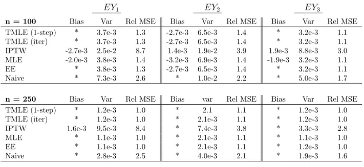
The first two tables (i.e., for Scenario I) present bias, relative efficiency and MSE estimates for the TMLE’s as well as each of the comparison estimators, for all three parameters specified above, i.e., those corresponding to EYd,

d = 1,2,3. For brevity, estimator performance for the other scenarios are presented only for EY1. There are only minor differences in the results for

the other parameter estimates.

Scenario I: Binary L(1) and A(1) Assigned at Random

In this scenario, we have L(0) as described above, A(0) and A(1) assigned at random and L(1) binary. Here the Naive estimator described above is consistent (though inefficient) and we include it as an interesting benchmark.

EY1 EY2 EY3

n = 100 Bias Var Rel MSE Bias Var Rel MSE Bias Var Rel MSE

TMLE (1-step) * 3.7e-3 1.3 -2.7e-3 6.5e-3 1.4 * 3.2e-3 1.1

TMLE (iter) * 3.7e-3 1.3 -2.7e-3 6.5e-3 1.4 * 3.2e-3 1.1

IPTW -2.7e-3 2.5e-2 8.7 1.4e-3 1.9e-2 3.9 1.9e-3 8.8e-3 3.0

MLE -2.0e-3 3.8e-3 1.4 -3.2e-3 6.9e-3 1.4 -1.9e-3 3.2e-3 1.1

EE * 3.8e-3 1.3 -2.7e-3 6.5e-3 1.4 * 3.2e-3 1.1

Naive * 7.3e-3 2.6 * 1.0e-2 2.2 * 5.0e-3 1.7

n = 250 Bias Var Rel MSE Bias var Rel MSE Bias Var Rel MSE

TMLE (1-step) * 1.2e-3 1.0 * 2.1 1.1 * 1.2e-3 1.0

TMLE (iter) * 1.2e-3 1.0 * 2.1e-3 1.1 * 1.2e-3 1.0

IPTW 1.6e-3 9.5e-3 8.4 * 7.4e-3 3.8 * 3.3e-3 2.8

MLE * 1.1e-3 1.0 * 2.1e-3 1.1 * 1.1e-3 1.0

EE * 1.1e-3 1.0 * 2.1e-3 1.1 * 1.2e-3 1.0

Naive * 2.8e-3 2.5 * 4.0e-3 2.1 * 1.9e-3 1.6

n = 500 Bias Var Rel MSE Bias Var Rel MSE Bias Var Rel MSE

TMLE (1-step) * 5.6e-4 1.0 * 1.1e-3 1.1 * 6.2e-4 1.1

TMLE (iter) * 5.6e-4 1.0 * 1.1e-3 1.1 * 6.2e-4 1.1

IPTW * 4.7e-3 8.4 -1.2e-3 3.4e-3 3.5 * 1.6e-3 2.8

MLE * 5.5e-4 1.0 * 1.1e-3 1.1 * 5.7e-4 1.0

EE * 5.6e-4 1.0 * 1.1e-3 1.1 * 6.2e-4 1.1

Naive -1.1e-3 1.4e-3 2.5 * 2.0e-3 2.1 * 9.6e-4 1.6

Table 1: Scenario I Data: Estimator performance for various sample sizes with Q and g correctly specified, for each of three estimated parameters. The estimates for the iterative TMLE were from the 5th iteration. Estimates were based on between 2000 and 5000 simulations, depending on sample size. An asterisk indicates an estimated bias<10−3_.

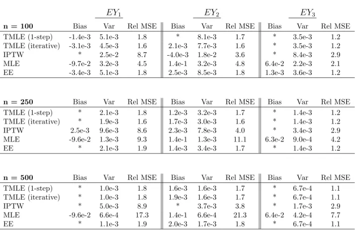
Scenario II: Binary L(1); A(1) Assigned in Response to L(1)

When L(1) is a confounder, the naive estimator is heavily biased and we omit it from the rest of the tables. For brevity we also only include the performance of the estimators for a single parameter, EY1. The results for

EY1 EY2 EY3

n = 100 Bias Var Rel MSE Bias Var Rel MSE Bias Var Rel MSE

TMLE (1-step) -1.4e-3 5.1e-3 1.8 * 8.1e-3 1.7 * 3.5e-3 1.2

TMLE (iterative) -3.1e-3 4.5e-3 1.6 2.1e-3 7.7e-3 1.6 * 3.5e-3 1.2

IPTW * 2.5e-2 8.7 -4.0e-3 1.8e-2 3.6 * 8.4e-3 2.9

MLE -9.7e-2 3.2e-3 4.5 1.4e-1 3.2e-3 4.8 6.4e-2 2.2e-3 2.1

EE -3.4e-3 5.1e-3 1.8 2.5e-3 8.5e-3 1.8 1.3e-3 3.6e-3 1.2

n = 250 Bias Var Rel MSE Bias Var Rel MSE Bias Var Rel MSE

TMLE (1-step) * 2.1e-3 1.8 1.2e-3 3.2e-3 1.7 * 1.4e-3 1.2

TMLE (iterative) * 1.9e-3 1.6 1.7e-3 3.0e-3 1.6 * 1.4e-3 1.2

IPTW 2.5e-3 9.6e-3 8.6 2.3e-3 7.8e-3 4.0 * 3.4e-3 2.9

MLE -9.6e-2 1.3e-3 9.3 1.4e-1 1.3e-3 11.1 6.3e-2 9.0e-4 4.2

EE * 2.1e-3 1.9 1.4e-3 3.4e-3 1.7 * 1.4e-3 1.2

n = 500 Bias Var Rel MSE Bias Var Rel MSE Bias Var Rel MSE

TMLE (1-step) * 1.0e-3 1.8 1.6e-3 1.6e-3 1.7 * 6.7e-4 1.1

TMLE (iterative) * 1.0e-3 1.8 1.9e-3 1.6e-3 1.7 * 6.7e-4 1.1

IPTW * 5.0e-3 8.9 * 3.7e-3 3.8 * 1.7e-3 2.9

MLE -9.6e-2 6.6e-4 17.3 1.4e-1 6.6e-4 21.3 6.4e-2 4.2e-4 7.7

EE * 1.1e-3 1.9 2.0e-3 1.7e-3 1.8 * 6.7e-4 1.1

Table 2: Scenario I Data: Estimator performance for various sample sizes with Q incor-rectly specified and g corincor-rectly specified, for each of the three parameters. Numbers of simulations for the various sample sizes ranged from 2000 to 5000. We exclude the Naive estimator from this table as the results should be quantitatively similar to those of the earlier simulations, since it does not depend on estimation ofQ(0).

Qc, gc

n= 100 n= 250 n= 500

Bias Var Rel MSE Bias Var Rel MSE Bias Var Rel MSE

TMLE (1-step) 3.0e-3 3.9e-3 1.3 * 1.3e-3 1.1 * 6.3e-4 1.1

TMLE (iter) 2.8e-3 3.9e-3 1.3 * 1.3e-3 1.1 * 6.3e-4 1.1

IPTW -1.8e-3 1.1e-2 3.9 * 4.6e-3 3.9 * 2.3e-3 4.0

MLE 1.2e-3 3.9e-3 1.3 -1.0e-3 1.3e-3 1.1 * 6.3e-4 1.1

EE 1.8e-3 3.8e-3 1.3 * 1.3e-3 1.1 * 6.3e-4 1.1

Qm, gc

n= 100 n= 250 n= 500

Bias Var Rel MSE Bias Var Rel MSE Bias Var Rel MSE

TMLE (1-step) 3.9e-3 4.5e-3 1.6 1.4e-3 1.7e-3 1.4 * 8.7e-4 1.5

TMLE (iter) 3.5e-3 4.5e-3 1.5 1.1e-3 1.7e-3 1.4 * 8.6e-4 1.5

IPTW 1.5e-3 1.1e-2 3.9 -2.4e-3 4.6e-3 3.9 -1.7e-3 2.3e-3 4.0

MLE -1.2e-1 2.8e-3 6.3 -1.3e-1 1.1e-3 14.6 -1.3e-1 5.7e-4 28.5

EE -1.2e-3 4.1e-3 1.4 -1.3e-3 1.6e-3 1.4 * 8.3e-4 1.4

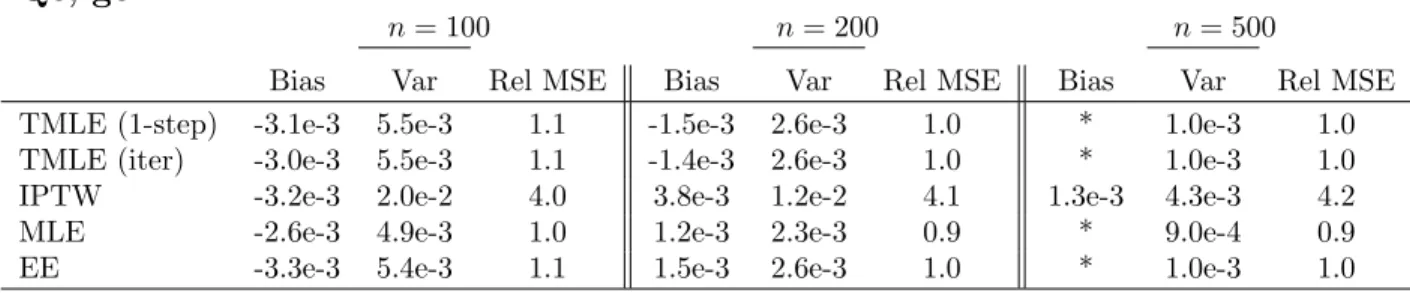
Table 3: Scenario II data: Performance of the various estimators in estimating a single parameter, EY1, for various sample sizes. ‘Qc, gc’: Q correctly specified, g correctly

Qc, gc

n= 100 n= 200 n= 500

Bias Var Rel MSE Bias Var Rel MSE Bias Var Rel MSE

TMLE (1-step) -3.1e-3 5.5e-3 1.1 -1.5e-3 2.6e-3 1.0 * 1.0e-3 1.0

TMLE (iter) -3.0e-3 5.5e-3 1.1 -1.4e-3 2.6e-3 1.0 * 1.0e-3 1.0

IPTW -3.2e-3 2.0e-2 4.0 3.8e-3 1.2e-2 4.1 1.3e-3 4.3e-3 4.2

MLE -2.6e-3 4.9e-3 1.0 1.2e-3 2.3e-3 0.9 * 9.0e-4 0.9

EE -3.3e-3 5.4e-3 1.1 1.5e-3 2.6e-3 1.0 * 1.0e-3 1.0

Qm, gc

n= 100 n= 200 n= 500

Bias Var Rel MSE Bias Var Rel MSE Bias Var Rel MSE

TMLE (1-step) -1.7e-3 5.2e-3 1.0 -1.9e-3 2.6e-3 1.0 * 1.1e-3 1.1

TMLE (iter) -1.7e-3 5.2e-3 1.0 -1.9e-3 2.6e-3 1.0 * 1.1e-3 1.1

IPTW 2.6e-3 2.0e-2 4.0 1.9e-3 1.0e-2 4.1 * 4.2e-3 4.1

MLE -7.0e-2 2.9e-3 1.5 -7.0e-2 1.5e-3 2.5 -7.0e-2 6.4e-4 5.5

EE -3.2e-3 5.1e-3 1.0 -2.2e-3 2.6e-3 1.0 * 1.1e-3 1.0

Table 4: Scenario III Data: Performance of the various estimators in estimating a single parameter,EY1, for various sample sizes. ‘Qc, gc’ means Q correctly specified, g correctly

specified, while ‘Qm’ means Q misspecified. Iterative TMLE estimates in this table were for the 3rd iteration. Asterisks indicate bias<10e-3.

Scenario III: Discrete L(1); A(1) Assigned in Response to L(1)

With discrete L(1) we modeled the binary factors QL(1)m similarly to the

way these factors were generated, i.e., using a hazard approach (see section 4.2). Thus each binary factor is modeled with logistic regression: as with the binary case, an initial estimate Q(0)_L(1)

m is obtained by logistic regression

(where this estimator could be correctly or incorrectly specified) and a cor-responding fluctuation function applied. See the appendix for the efficient influence curve for these individual binary factors, which imply the form of the fluctuation functions Qn,L(1)m() used in the targeting step.

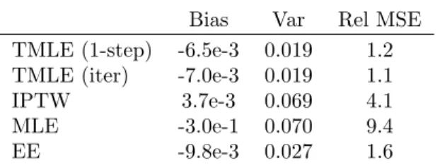
Small Sample Results

We also simulated data under scenario III above for a sample size of 30. We anticipated efficiency differences (if any) between the iterative and one-step TMLE’s would show up at this very small sample size (see Discussion

sec-Qc, gc

Bias Var Rel MSE

TMLE (1-step) -0.016 0.023 1.4 TMLE (iter) -0.021 0.022 1.4 IPTW 1.4e-3 0.067 4.0 MLE -0.035 0.021 1.3 EE -0.027 0.021 1.3 Qm, gc

Bias Var Rel MSE

TMLE (1-step) -6.5e-3 0.019 1.2 TMLE (iter) -7.0e-3 0.019 1.1

IPTW 3.7e-3 0.069 4.1

MLE -3.0e-1 0.070 9.4

EE -9.8e-3 0.027 1.6

Table 5: Scenario III Data, atn= 30: Performance of the various estimators in estimat-ing a sestimat-ingle parameter, EY1. ‘Qc, gc’ means Q correctly specified, g correctly specified,

while ‘Qm’ means Q misspecified. Iterative TMLE estimates in this table were for the 4th iteration.

tion). We saw no significant difference in the variance of these two estimators, however. The performance of the TMLE’s at this sample size is remarkable, particularly under model misspecification, and we felt these results warranted a separate table.

4.4

Discussion

Relative efficiency for the ML estimator is almost always _. 1. The semi-parametric efficiency bound does not apply in general to that of an estimator based on a parametric model. Even so, when Q is correctly specified, the variance of the ML estimator appears to be very close to the semi-parametric efficiency bound when n≥200.

Of particular note is that the TMLE, EE and MLE estimators are already very close to the efficiency bound at n = 250 under Qc in the binary L(1) case. Further, the reduction in bias in going to n = 500 is small in absolute terms.

Even more noteworthy is the performance of the TMLE’s at the small sample size of 30 for the scenario III simulations (discreteL(1)). Bias and variance of both estimators are better when Q(0) is misspecified. Misspecification in this case consisted in setting Logit(QL(2)) = 3∗L(1) (compare with the true data

generating function), but using correct specification for QL(1). With Q(0)

misspecified, the bias of both TMLE’s is quite small and the variance is very close to the efficiency bound. The better performance under misspecification can be understood by noting that under correct model specification, many more parameters of the model need to be fit. We expect that asymptotically, there is a gain in efficiency of the TMLE’s if Q(0) _{is consistently estimated,}

but these simulations show that a parsimonious, though incorrect, model as initial estimator can have distinct advantages in the double robust TMLE at small sample sizes, even over using the correct initial model.

The effect is still noticeable at sample size 100 in the discreteL(1) case. There we also see lower bias of the TMLE’s under incorrect model specification than under correct model specification. This phenomenon is not present in the scenario II simulations however.

The advantage of the TMLEs’ being substitution estimators also becomes apparent in these small sample results: atn = 30, many times the estimating equation and IPTW estimators gave estimates outside the range [0,1] (note that the parameters here are always in [0,1]), and this also contributes to their higher variance.

In general, under incorrect specification of Q we do not expect any of the estimators that estimateQ0to beasymptotically efficient except for the MLE,

which used a much simpler model than the true model and therefore could easily achieve a lower variance bound. Misspecification of Q in all cases was implemented by misspecifying Q(0)_L(2) but correctly specifying QL(1). Thus

under Qm, gc the MLE will be biased but the TMLE and EE estimators are double robust and therefore still asymptotically unbiased under correct specification of g. Under the scenarios simulated here g is expected to be known and we therefore omitted simulations in which g is misspecified; the latter will of course result in bias of the IPTW estimator. Scenarios in which

g is not known, or not completely known are also quite plausible, however; e.g., one can easily imagine settings in which assignment of A(0) and/or

A(1) was not done in complete accordance with a defined treatment rule. Nevertheless, even in these cases, with A(0) randomized and L(1) discrete or binary, non-parametric estimation of g would not be difficult. If A(0) is

a function of L(0) then some smoothing will be required for the estimate of

g(A(0) |L(0)) and model misspecification is likely to arise.

The two versions of TMLE we’ve implemented (one-step and iterative) typ-ically agree in their estimate of the parameter to within 1%, and in many cases to within quite a bit less than this. The choice in implementation will depend on one’s data. For example, with two time points and a single inter-mediate covariate L(1) with a small number of discrete levels, the one-step estimator is conceptually easier to implement than the iterative approach. As the number of estimated factors increases (either from having multiple time points, multiple covariates in L(j), 1 < j < K, or both), the iterative method may become the more practical programming choice.

Also noteworthy is that the one-step TMLE requires estimation of two ’s in the binary L(1) case and four ’s in the discrete L(1) case. For the gen-eral data structure (L(0), A(0), ...L(K), A(K), L(K+ 1)) where intermediate factor L(j) has tj levels, the number of ’s the one-step estimator must fit is

PK+1

j=1 (tj −1). In contrast, the iterative TMLE performs a fitting of that

is independent of K and tj. (Though a new round of fitting occurs for each

iteration, the bulk of the fitting occurs in the first iteration.) We thus expect at least a small efficiency advantage for the iterative method. We have not observed this advantage in the current simulation study even for a sample size as low as 30, though we still expect it to appear as K and/ortj increase.

Appendix I: Confirming Correct

Implementa-tion of the TMLE Methods

Implementing TMLE in longitudinal settings is not a trivial exercise. How-ever, there are several checks one can use to ensure the estimator is being correctly implemented. For example, if one is simulating data, one can check the double-robust property, i.e., make sure the estimator goes to the truth (as n increases) under misspecification of eitherQ org (but not both at the same time).

If both Q and g are correctly specified, the variance of the TMLE’s should achieve the semi-parametric efficiency bound well before n= 1000 under any of the three data scenarios presented here.

If one is using the method on real data to estimate a parameter of inter-est, simulation from a proposed Qn can still be performed and the

double-robustness property checked as above. An equally important check—which can be performed on a real data set—is that the estimator solves the empiri-cal mean of the efficient influence curve; i.e. one checks thatPnD∗(Q∗, gn)) =

0. In our simulations the one-step estimator typically yielded values of

|PnD∗(Q∗, gn))| . 10−10. For the iterative approach, successive iterations

should produce decreasing values of |PnD∗|. An illustration of this is given

in Table 6, which shows median values of |PnD∗| from two of our simulation

scenarios.

Scenario II, n = 250, Qc, gc

One-step 1st 2nd 3rd 4th

1.3e-10 5.0e-04 2.5e-05 1.2e-06 5.6e-08

Scenario III, n = 200, Qc, gc

One-step 1st 2nd 3rd 4th

1.2e-10 3.9e-04 1.4e-05 5.2e-07 2.1e-08

Table 6: Median values of|PnD∗| for the one-step and iterative approaches in

estimat-ing EY1 for two of the data scenarios examined. Scenario II data was based on 5000

simulations; scenario III, 500 simulations. BothQand gwere correctly specified in these simulations. Values for the one-step TMLE and the first four iterations of the iterative TMLE are presented.

Appendix II: Formulas for Efficient Influence

Curve and Clever Covariates for discrete

L(1)

In the following, D₁∗_,t indicates the efficient influence curve for thetth binary indicator of L(1), t= 0,1,2,3, andP a(L(1)) = (L(0), A(0)). We have

D∗_1,0(O) = I(_gA₍(0)=_d0(Ld0₍₀₎₎(L_|(0)))_X) × {E(Yd |L(1) = 0, P a(L(1)))−

P

m>0E[Yd |L(1) =m, P a(L(1))]P(L(1) =m |L(1)>0, P a(L(1)))}×

where, e.g., P(L(1) = 2|L(1)>0, P a(L(1))) = P(L_P(1)=2_(L(1),L_>(1)_{0|P a}>0₍|_LP a₍₁₎₎₎(L(1))) = ₁₋P_P(L_(L(1)=2)₍₁₎₌₀|_|P a_{P a}(₍L_L(1))₍₁₎₎₎ = P(L(1)=2|L(1)≥2,P a(L(1))) Q s<2[1−P(L(1)=s|L(1)≥s,P a(L(1)))] 1−P(L(1)=1|P a(L(1)) =P(L(1) = 2|L(1)≥2, P a(L(1))) [1−P(L(1) = 1|L(1) ≥1, P a(L(1)))], and P(L(1) = 3|L(1)>0, P a(L(1))) =P(L(1) = 3|L(1)≥3, P a(L(1)))Q2_s=1[1−P(L(1) =s|L(1)≥s, P a(L(1)))] = 1∗Q2_s=1[1−P(L(1) =s |L(1) ≥s, P a(L(1)))]. Similarly, D∗_1,1(O) = I(_gA₍(0)=_d0(Ld0₍₀₎₎(L_|(0)))_X) × {E(Yd |L(1) = 1, P a(L(1)))− P m>1E[Yd |L(1) =m, P a(L(1))]P(L(1) =m |L(1)>1, P a(L(1)))}× {I(L(1) = 1)−I(L(1) ≥1)E[I(L(1) = 1)|L(1)≥1, P a(L(1))]}, and E[I(L(1) =m)|L(1) ≥m, P a(L(1))]≡P(L(1) =m |L(1) ≥m, P a(L(1))).

D∗_1,2(O) is similar, but D₁∗_,3(O) = 0 since

I(L(1) = 3)−I(L(1) ≥3)E[I(L(1) = 3)|L(1)≥3, P a(L(1))]

=I(L(1) = 3)−I(L(1) = 3)∗E[I(L(1) = 3)|L(1)≥3, P a(L(1))] =I(L(1) = 3)−I(L(1) = 3)∗P[L(1) = 3|L(1)≥3, P a(L(1))] =I(L(1) = 3)−I(L(1) = 3)∗1 = 0.

Thus the efficient influence curve for EYd is

D∗(O) =D₀∗(O) +

3 X

t=0

with D∗₀(O) and D∗₂(O) exactly as given in Theorem 1.

The expression for clever covariate CL(1,j) follows immediately from D1∗,j as

simply the IPCW term times the first bracketed term. So, for example,

CL(1,2) would be CL(1,2) = I(A(0)=d0(L(0))) g(d0(L(0))|X) × {E(Yd |L(1) = 2, P a(L(1)))− P m>2E[Yd |L(1) =m, P a(L(1))]P(L(1) =m |L(1) >2, P a(L(1)))}.

Computing Empirical Mean of Efficient Influence Curve

for Iterative TMLE

Determining whether the TMLE ofEYd, Ψd(Q∗n), solves the efficient influence

curve proceeds as follows. For each row of the original data (i.e., data frame for which each row is one subject/observation), the updated estimates of

QL(1,t), t = 0,1,2,3, and QL(2) are computed. For example, for row i, under

rule d, we have

EQ∗[(Y_d)_i] =E_Q∗(Y |L(1) = 0,A(1)¯ _i =d( ¯L), L(0)_i)×λ_Q∗(0|P a(L(1))_i)+

EQ∗(Y |L(1) = 1,A(1)¯ _i=d( ¯L), L(0)_i)×λ_Q∗(1|P a(L(1))_i)[1−λ_Q∗(1|P a(L(1))_i)]+

EQ∗(Y |L(1) = 2,A(1)¯ _i=d( ¯L), L(0)_i)×λ_Q∗(2|P a(L(1))_i)Q

s<2[1−λQ∗(s|P a(L(1))_i)]+

EQ∗(Y |L(1) = 3,A(1)¯ _i=d( ¯L), L(0)_i)×λ_Q∗(3|P a(L(1))_i)Q

s<3[1−λQ∗(s|P a(L(1))i)],

where λQ∗(s | P a(L(1))_i) = P_Q∗(L(1) = s | L(1) ≥ s, L(0)_i, A(0)_i =

d(L(0))), and EQ∗(Y | ...) and λ_Q∗(s | ...) are the updated estimates, Q∗

L(2)

and Q∗_L(1,s), respectively.

D∗₀(Oi)(Q∗, g0) is then given byEQ∗[(Y_d)_i]−Ψ_d(Q∗

n).

D∗_1,j(Oi)(Q∗, g0) are computed according to the formulas given in the previous

section with all the terms E(Y | ...) and P(L(1) = m | ...) replaced with

EQ∗(Y |...), P_Q∗(L(1) =m|...) as shown in D∗

0(Oi)(Q∗, g0) above.

D∗₂(Oi)(Q∗, g0) is given byI_g( ¯₍A_{d( ¯}i=_L)d_|( ¯_XL_i))₎×{Yi−EQ∗(Y |L(1)_i,A¯(1)_i =d( ¯L), L(0)_i)}.