Repositorio Institucional de la Universidad Autónoma de Madrid
https://repositorio.uam.es
Esta es la
versión de autor
del artículo publicado en:
This is an
author produced version
of a paper published in:
Pattern Recognition Letters 32.11 (2011): 1567 – 1571
DOI:
http://dx.doi.org/10.1016/j.patrec.2011.04.007
Copyright:
© 2011 Elsevier B.V.
El acceso a la versión del editor puede requerir la suscripción del recurso
Access to the published version may require subscription
On the Equivalence of Kernel Fisher Discriminant Analysis and Kernel
1
Quadratic Programming Feature Selection
2
I. Rodriguez-Lujana,∗, C. Santa Cruza, R. Huertab 3
a
Departamento de Ingenier´ıa Inform´atica and Instituto de Ingenier´ıa del Conocimiento, Universidad Aut´onoma de Madrid,
4
28049 Madrid, Spain.
5
bBioCircuits Institute, University of California San Diego, La Jolla CA 92093-0404, USA. 6
Abstract
7
We reformulate the Quadratic Programming Feature Selection (QPFS) method in a kernel space to obtain a vector which maximizes the quadratic objective function of QPFS. We demonstrate that the vector obtained by Kernel Quadratic Programming Feature Selection is equivalent to the Kernel Fisher vector and, therefore, a new interpretation of the Kernel Fisher Discriminant Analysis is given which provides some computational advantages for highly unbalanced datasets.
Keywords: Kernel Fisher Discriminant, Quadratic Programming Feature Selection, Feature Selection,
8
Kernel Methods.
9
1. Introduction
10
Identifying a proper representation of data is a problem of growing importance in machine learning
11
because of the increasing size and dimensionality of real-world datasets. Linear feature selection and
extrac-12
tion methods, such as Principal Component Analysis (PCA) (Jolliffe, 2002), Canonical Correlation Analysis
13
(CCA) (Afifi and Clark, 1999) and Linear Discriminant Analysis (LDA) (Fukunaga, 1972), are preferable
14
due to their computational speed and simplicity but for most real-world data they are not complex enough.
15
They are conducted in the original space and cannot handle nonlinear relationships in the data. One option
16
to tackle this problem is making use of kernel methods (Shawe-Taylor and Cristianini, 2004) which maps the
17
data from an original space to afeature spaceFvia a (nonlinear) mapping Φ :Rl−→ F. The dot-product in
18
∗Corresponding author. Tel: +34 91 497 2339; fax: +34 91 497 2334
Email addresses: [email protected](I. Rodriguez-Lujan),[email protected](C. Santa Cruz),
the feature spaceF is defined by a Mercer kernel (Mercer, 1909)K:Rl×Rl−→Rand, the reformulation of
19
traditional linear methods using only dot-products of training samples yields implicitly a nonlinear method
20
in the input space. Examples of these methods are Kernel-PCA (Schlkopf et al., 1998), Kernel-CCA (Lai
21
and Fyfe, 2000) and the Kernel Fisher Discriminant (Mika et al., 1999).
22
In this work, we adapt our previous feature selection method QPFS (Rodriguez-Lujan et al., 2010) in a
ker-23
nel space to provide a vector in the kernel space which maximizes the quadratic objective function. Using
24
the Quadratic Program representation of the KFD proposed by (Mika et al., 2000), we demonstrate the
25
equivalence between KFD and KQPFS. This equivalence provides a new interpretation of the Kernel Fisher
26
vector which only depends on the kernel matrix and the labels of training samples making unnecessary the
27
kernelized between and within class scatter matrices calculation. We also study the training cost of both
28
algorithms.
29
The present manuscript is organized as follows. Section 2 reformulates the Kernel Fisher Discriminant
Anal-30
ysis to a Quadratic Program. Section 3 presents the formulation of the QPFS algorithm in a kernel space,
31
including a regularized version to overcome numerical problems. Section 4 shows the equivalence between
32
KFD and KQPFS and how this equivalence provides a new interpretation of KFD. Section 5 compares their
33
computational complexity. Finally, Section 6 shows the empirical equivalence of KFD and KQPFS in several
34
well-known artificial and real-world datasets. The runtime of both methods as a function of the class label
35
prior probabilities is also provided.
36
37
38
2. Kernel Fisher Discriminant
39
Let X1 = {x11, . . . , x1l1} and X2 = {x 2
1, . . . , x2l2} be samples from two different classes, xi ∈ R
d and
40
X =X1∪ X2the complete set ofl(l=l1+l2)training samples. And lety∈ {−1,1}lbe the vector with the 41
corresponding labels.
42
The Kernel Fisher Discriminant (KFD) consists on finding nonlinear directions by first mapping the data
43
nonlinearly into the feature space F and computing Fisher’s linear discriminant there (Mika et al., 1999).
Specifically, let Φ :Rd −→ F be the mapping function to the kernel space andK(x, y) =<Φ(x),Φ(y) > 45
the Mercer kernel which defines the dot-product in F. To find the linear discriminant in F we need to
46 maximizing, 47 J(w) = w TSΦ Bw wTSΦ Ww (1) 48 wherew∈ F andSΦ B andS Φ
W are the corresponding between and within scatter matrices inF, i.e.
49 SBΦ = (mΦ1 −m Φ 2)(m Φ 1 −m Φ 2)T 50 SWΦ = X i=1,2 X x∈χi (Φ(x)−mΦi)(Φ(x)−mΦi )T 51 withmΦ i = 1 li Pli j=1Φ(xij). 52 53 54
Finding a solution to Equation 1 in the kernel space F requires to reformulate it in terms of only dot
55
products of the input patterns (Mika et al., 1999). From the theory of reproducing kernels (Saitoh, 1988),
56
any solutionw∈ F must lie in the span of all training samples inF. Thereforew can be expressed as,
57 w= l X i=1 αiΦ (xi) 58
Therefore, maximizing Equation 1 is equivalent to maximize
59 J(α) = α TM α αTN α 60 61 being 62
M = (M1−M2)(M1−M2)T 63 (Mi)j = 1 li li X k=1 K(xj, xik) 64 N = X j=1,2 Kj(I−1lj)K T j 65
whereKj is a N×lj matrix with (Kj)nm=k(xn, xjm),Iis the identity matrix and 1lj the matrix with
66
all entries 1
lj.
67
This problem can be solved by finding the leading eigenvector ofN−1M or computingα∗
KFD=N −1(M
2− 68
M1). In the last case, some kind of regularization is needed because the problem is ill-posed (Tikhonov and 69
Arsenin, 1977): the dimension of the feature space is usually larger than the number of training samples,
70
which makes matrixNnot positive. Regularization functions askαk2,kwk2and others have been proposed in 71
(Mika et al., 1999; Friedman, 1989; Hastie et al., 1993). In (Mika et al., 1999), the matrixNis approximated
72
byNµ=N+µNIbeing µN the minimum value which makesN positive definite.
73
3. Kernel Quadratic Programming Feature Selection
74
The proposed QPFS method (Rodriguez-Lujan et al., 2010) consists on minimizing a multivariate
75
quadratic function subjected to linear constraints as follows,
76 min x 1 2x TQx−FTx (2) 77 s.t. xi≥0 ∀i= 1. . . M 78 kxk1= 1. 79
Wherexis and-dimensional vector, Q∈Rd×d is a symmetric positive semidefinite matrix, andF is a
80
vector inRd with non-negative entries. Q represents the similarity among variables (redundancy), andF 81
measures how correlated each feature is with the target class (relevance). The components of the solution
82
vectorx∗
represents the weight of each feature, and we chose to normalize the contribution of each feature
to the cost function. Thus, the aim of Equation 3 is to select those features which provide a good tradeoff
84
between relevance and redundancy for the classification task.
85
The formulation of Equation 3 in a kernel space is not straightforward. For some kernels, it is not
86
possible to give a weight to each feature in the kernel space due to its potential infinite dimension. However,
87
maintaining the goal of redundancy minimization of the features and relevance maximization of each feature
88
with the target class, the Equation 3 can be adapted to find an optimal directionwto project the data into
89
the kernel space. As before, let Φ be the nonlinear mapping to the feature spaceF then, the adapted QPFS
90
objective function is defined as,
91 min x 1 2w TQΦ w− FΦT w (3) 92
where QΦ is the redundancy among features in the kernel space, FΦ is the relevance of each feature
93
with the target class in the kernel space. Thus Equation 3 represents a feature extraction method, KQPFS,
94
instead of a feature selection technique as the original QPFS method.
95
In the original QPFS approach, correlation and mutual information were considered as similarity
mea-96
sures of redundancy and relevance. For our problem in Equation 3, a linear dependence must be applied
97
becausewinduces a linear projection of the data. Intuitively, it is possible to adapt mutual information or
98
correlation in the kernel space. However, the mapping function Φ is usually implicit and the dimension of
99
the kernel spaceF may be infinite forcing the search of a basis set in the kernel space. If instead of mutual
100
information or correlation, the covariance is used as similarity measure, the KQPFS formulation does not
101
require the presence of an explicit basis in the kernel space. More precisely, theQΦ and FΦ matrices are 102 defined as follows, 103 QΦ = X x∈X Φ(x)−mΦ Φ(x)−mΦT 104 FΦ = X x∈X (yx−my) Φ(x)−mΦ 105
wheremΦandmy are the mean value of the training samples and the training labels, respectively. That
is, 107 mΦ = 1 l X x∈X Φ(x) 108 my = 1 l l X i=1 yi . 109
Again, we first need a formulation of Equation 3 in terms of only dot products of input patterns and
110
applying the theory of reproducing kernels (Saitoh, 1988),wis represented asw=Pl
i=1αiΦ (xi). Therefore,
111
Equation 3 can be formulated as the minimization of functionG(α),
112 G(α) = 1 2α TK(I−1 l)Kα−yT(I−1l)Kα (4) 113
whereI is thel-dimensional identity matrix and 1l is al-dimensional square matrix with all entries 1l.
114
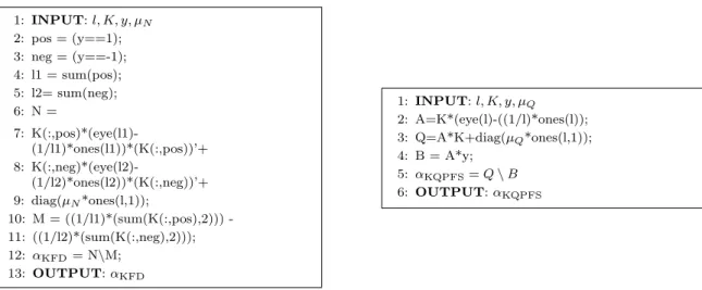
Let QK =K(I−1l)K and FK = K(I−1l)y, the optimal value of α∗KQPFS is obtained making the 115
gradient ofG(α) equals to zero,
116
αKQPFS∗ = (QK)
−1 FK
117
If theQK matrix is invertible, the formulation of the optimal direction is straightforward,
118 α∗KQPFS = (QK) −1 FK 119 = K−1(I−1l)−1K−1K(I−1l)y 120 = K−1y 121
Unfortunately, the matrix QK =K(I−1l)K is always singular because its rank is upper-bounded by
122
the rankl−1 of matrix (I−1l). Therefore, following (Mika et al., 1999), a multiple of the identity matrix
123
is added toQK matrix: Qµ=QK+µQI.
124
ReplacingQK byQµ in Equation 4, we obtain the regularized version of KQPFS,
125 Gµ(α) = 1 2α T(Q K+µQI)α−FKTα 126
which is equivalent to, 127 Gµ(α) = 1 2α TQ Kα−FKTα+ µQ 2 kαk 2 . (5) 128
And the regularized KQPFS direction is given by,
129 α∗ KQPFS= (QK+µQI) −1 FK (6) 130
µQ is the minimum value which makes Qµ positive definite. A process to estimate the parameter µQ is
131
needed. The KQPFS solution obtained in Equation 6 has an easy interpretation as the projection direction
132
which minimizes the covariance among features in the kernel space and maximizes the covariance of each
133
feature in the kernel space with the target class. Moreover, the expression of such direction is quite simple
134
depending only on the kernel matrixKand the class labelsy.
135
4. Equivalence of KFD and KQPFS
136
In this section we will demonstrate that the optimal solution of KQPFS is equivalent to the solution of
137
KFD when the same regularization criteria is applied in both cases. Without loss of generality, we will use
138
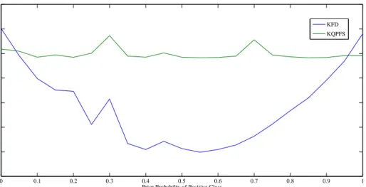
the regularization defined in Sections 2 and 3. It is straightforward to show that the following proof is also
139
valid for other regularization functions.
140
As shown in (Mika et al., 2000), the KFD can be reformulated as the following quadratic programming
141 problem, 142 min α α TN α+CP(α) (7) 143 Subject to: 144 αT(M1−M2) = 2 (8) 145
where P(α) is a regularization term which makes explicit theN regularization and C∈Rthe
regular-146
ization constant. It can be shown (Mika et al., 2000) that solving the problem given in Equations 7 and 8
147
is equivalent to optimize,
min α,b,ξkξk 2+ CP(α) (9) 149 Subject to: 150 Kα+−→1b = y+ξ (10) 151 −→ 1T i ξ = 0 fori= 1,2 (11) 152
being −→1 ∈Rl a vector with all entries 1 and−→1
iRl binary vectors with j-th entry equals to 1 if the j-th
153
sample belongs to class iand 0 otherwise. The quadratic optimization problem defined in Equations 9-11
154
can be understood as the minimization of the variance of the data along the projection and the maximization
155
of the distance between the average outputs for each class at the same time.
156
Replacing N by Nµ in Equation 7, the regularization term P(α) is equal to kαk2, the regularization
157
constantC isµN and the regularized quadratic problem in Equations 9-11 is reformulated as,
158 min α,b,ξkξk 2+ µNkαk2. (12) 159 Subject to: 160 Kα+−→1b = y+ξ (13) 161 −→ 1T i ξ = 0 fori= 1,2 (14) 162
Proposition 1. Given µN ∈ R and let µN = µQ, any optimal solution (α∗, b∗, ξ∗) to the optimization
163
problem (12-14) is also optimal for (5) and vice versa.
164
Proof. Working outξin the constraint given in Equation 14 leads to
165
ξ(α, b) =Kα+−→1b−y . 166
By expandingkξ(α, b)k2 the optimization problem of Equation 12 is reformulated as 167 min α,b{α TKKα−lb2−2 yTKα+yTy+µNkαk2} 168
subject to: 169 −→ 1T iξ(α, b) = 0 fori= 1,2 170
The value of bcan be expressed as a function ofαusing the second constraint:
171
b(α) =−1
l1lKα+ 1ly . (15)
172
Therefore, we have an optimization problem with no constraints:
173 minα {αTKKα−l(b(α)) 2 (16) 174 −2yTKα+yTy+µNkαk2}. (17) 175
Then, substitutingb(α) in Equation 17 by the value obtained in Equation 15 we obtain
176 minα {αTK(I−1l)Kα 177 −2yT(I−1l)Kα+ µN 2 kαk 2+ D} (18) 178
withDbeing a constant. It follows that the minimum value of Equation 18 is the same as the obtained for
179
the objective function of the regularized KQPFS (Equation 5) whenµN =µQ.
180
2
181
This equivalence provides a new solution of the Fisher direction which not depends explicitly on the
182
un-intuitive kernelized within scatter matrix N (Equation 6). Moreover, the Fisher solution has a simple
183
interpretation as the direction which minimizes the covariance among features and maximizes the covariance
184
of each feature with the target class.
185
5. Computational Cost Comparison
186
In this section we study the computational cost of KFD and KQPFS to determine whether it is possible
187
to get any computational advantage from the new KFD formulation as the kernelization of QPFS. Even
188
though several algorithms have been proposed to speed up KFD (Cai, 2007; Mika, 2001; Xiong et al., 2004)
189
we are interested in analyzing an equivalent problem to the KQPFS as given in Equation 6. Let us to obtain
190
thestandard KFD solution as α∗
KFD = (Nµ)−1(M1−M2) where matrices Nµ, M1 and M2 are defined in 191
1: INPUT:l, K, y, µN 2: pos = (y==1); 3: neg = (y==-1); 4: l1 = sum(pos); 5: l2= sum(neg); 6: N = 7: K(:,pos)*(eye(l1)-(1/l1)*ones(l1))*(K(:,pos))’+ 8: K(:,neg)*(eye(l2)-(1/l2)*ones(l2))*(K(:,neg))’+ 9: diag(µN*ones(l,1)); 10: M = ((1/l1)*(sum(K(:,pos),2))) -11: ((1/l2)*(sum(K(:,neg),2))); 12: αKFD= N\M; 13: OUTPUT:αKFD 1: INPUT:l, K, y, µQ 2: A=K*(eye(l)-((1/l)*ones(l)); 3: Q=A*K+diag(µQ*ones(l,1)); 4: B = A*y; 5: αKQPFS=Q\B 6: OUTPUT:αKQPFS
Figure 1: MATLAB code of KFD (left) and KQPFS (right) algorithms.
Section 2. Figure 1 shows the MATLAB code for both methods. The number of float-point operations
192
needed by KFD is 4l (lines 2-5),l2
1+l22+l2+ 2l(l21+l22) + 3l2 (lines 6-9), l2+ 3l (lines 10-11) and O(l3) 193
(line 12) which makes a total cost of O(l3) + 2l(l2
1+l22) + 5l2+l21+l22+ 7l operations. In the case of the 194
KQPFS algorithm,l2+l3 operations are needed in line 2, 2l2+l3 in line 3, l2 in line 4 and O(l3) in line 5 195
that is, a total cost ofO(l3) + 2l3+ 4l2 float-point operations. As the line 12 of KFD and line 5 of KQPFS
196
work with dimensionality equivalent matrices, we will suppose that the cost of these lines is the same in
197
both cases therefore, we obtain that KQPFS is computationally faster than the proposed version of KFD if
198
(l2
1+l22)(2l+ 1) + 5l2+ 7l ≫2l3+ 4l2. The inequality is satisfied when the prior distributions of the class 199
labels are highly unbalanced i.e., whenl1→l orl2→l. Summing up, the KFD cost depends on the prior 200
distribution of classes and KQPFS is more efficient for highly unbalanced classification problems.
201
6. Experiments
202
A theoretical proof of the equivalence between KFD and KQPFS has been given in Proposition 1 and in
203
this section we show that the numerical solutions given by KFD and KQPFS provide the same projection
204
direction.
205
We followed part of the experimental setup described in (Mika et al., 1999): for KFD and KQPFS we
206
used Gaussian kernels and the regularized matricesNµandQµas described in Sections 2 and 3, respectively.
Thirteen artificial and real world datasets were considered from the R¨atsch benchmark repository1. Some 208
of these datasets were not binary so they were transformed into two-classes problems and all of them were
209
partitioned into 100 pairs of training and test sets (about 60%:40%).
210
The experiments require to estimate two parameters, the width of the Gaussian kernelK(x, y) =ekx−σyk2
211
and the regularization parameter µN of the within class scatter matrix N in KFD (see section 2). The
212
procedure to estimate these parameters consists on running 5-fold cross validation on the first five realizations
213
of the training sets and taking the model parameter to be the median over the five estimates. The value of
214
these parameters is known (Mika et al., 1999). Note that the equivalence of KQPFS and KFD holds when
215
the same regularization form and regularization constant is applied in both cases. Therefore, there is no
216
need to estimate the KQPFS regularization parameterµQ.
217
The empirical equivalence of KFD and KQPFS has been confirmed measuring the cosine between the
218
solutions α∗
KFD and α ∗
KQPFS. Ideally, the value of the cosine should be close to 1 or to −1 which means 219
parallel directions. In all the datasets, the cosine of both directions was 1 for every training set.
220
Finally, let us provide numerical results of the KFD and KQPFS complexity analyzed in Section 5. The
221
experiment consists on modifying the prior probability of one of the classes, without loss of generality the
222
class of positive labels, and compare the runtime of KFD and KQPFS codes (Figure 1). The regression
223
dataset Abalone available in the LIBSVM repository (Chang and Lin, 2001) was used. The dataset has 4177
224
samples (l) in a 8-dimensional space. To carry out the experiments, the samples were arranged in ascending
225
order according to the regression variable and the prior probability of the positive class p1 was modified 226
from 0 to 1 with a stepwise of 0.05. A pattern is assigned to the positive class if it is among the first p1l 227
patterns. Figure 2 shows the runtime in training as a function of the prior probability of the positive class.
228
As expected, the KFD algorithm cost is dependent on the class prior probabilities being faster than KQPFS
229
except when the class distributions are highly unbalanced. The KQPFS complexity is independent on the
230
prior distributions.
231
0 0.1 0.2 0.3 0.4 0.5 0.6 0.7 0.8 0.9 1 18 19 20 21 22 23 24 25
Prior Probabilty of Positive Class
Training Time (Seconds)
KFD KQPFS
Figure 2: Abalone. Training time in seconds for the KFD and KQPFS algorithms.
7. Conclusions
232
This paper reformulates the Quadratic Programming Feature Selection (QPFS) method to obtain an
233
optimal projection direction in a kernel space (KQPFS). The projection direction given by KQPFS is
equiv-234
alent to those obtained by the Kernel Fisher Discriminant (KFD) which leads to a new interpretation of the
235
KFD vector as the direction which minimizes the covariance among features and maximizes the covariance
236
of each feature with the target class in the kernel space. This equivalence provides a new solution for KFD
237
disregarding the explicitly dependence on the kernelized between and within scatter matrices. In addition, a
238
more efficient computation of the Kernel Fisher direction is proposed when the classes are highly unbalanced.
239
Acknowledgments
240
I.R.-L. is supported by an FPU grant from Universidad Aut´onoma de Madrid, and partially supported
241
by the Universidad Aut´onoma de Madrid-IIC Chair. R.H. acknowledges partial support by ONR
N00014-242
07-1-0741, NIDCD 1R01DC011422-01 and JPL-1396686.
243
References
244
Afifi, A. A., Clark, V., 1999. Computer-Aided Multivariate Analysis, 2nd Edition. Chapman & Hall, Ltd., London, UK, UK. 245
Cai, D., 2007. Efficient kernel discriminant analysis via spectral regression. Tech. rep. 246
Chang, C.-C., Lin, C.-J., 2001. LIBSVM: a library for support vector machines. Software available at 247
http://www.csie.ntu.edu.tw/ cjlin/libsvm.
Friedman, J. H., 1989. Regularized discriminant analysis. Journal of the American Statistical Association 84 (405), pp. 165–175. 249
Fukunaga, K., 1972. Introduction to Statistical Pattern Recognition. New York, San Francisco, London: Academic Press. 250
Hastie, T. J., Tibshirani, R. J., Buja, A., 1993. Flexible discriminant analysis by optimal scoring. Tech. rep., AT&T Bell 251
Laboratories. 252
Jolliffe, I. T., 2002. Principal Component Analysis. Springer, New York, NY, USA. 253
Lai, P. L., Fyfe, C., 2000. Kernel and nonlinear canonical correlation analysis. Int. J. Neural Syst. 10 (5), 365–377. 254
Mercer, J., 1909. Functions of positive and negative type, and their connection with the theory of integral equations. Philo-255
sophical Transactions of the Royal Society, London 209, 415–446. 256
Mika, S., 2001. An improved training algorithm for kernel fisher discriminants. In: In Proceedings AISTATS 2001. Morgan 257
Kaufmann, pp. 98–104. 258
Mika, S., Rtsch, G., Mller, K.-R., 2000. A mathematical programming approach to the kernel fisher algorithm. In: Leen, T. K., 259
Dietterich, T. G., Tresp, V. (Eds.), NIPS. MIT Press, pp. 591–597. 260
Mika, S., Rtsch, G., Weston, J., Schlkopf, B., Mller, K.-R., 1999. Fisher discriminant analysis with kernels. 261
Rodriguez-Lujan, I., Huerta, R., Elkan, C., Cruz, C. S., August 2010. Quadratic programming feature selection. J. Mach. 262
Learn. Res. 99, 1491–1516. 263
Saitoh, S., 1988. Theory of Reproducing Kernels and its Applications. Longman Scientific&Technical, Harlow, England. 264
Schlkopf, B., Smola, A., Mller, K.-R., 1998. Nonlinear component analysis as a kernel eigenvalue problem. Neural Comput. 265
10 (5), 1299–1319. 266
Shawe-Taylor, J., Cristianini, N., 2004. Kernel Methods for Pattern Analysis. Cambridge University Press, Cambridge, UK. 267
Tikhonov, A. N., Arsenin, V. Y., 1977. Solutions of Ill-posed problems. W.H. Winston. 268
Xiong, T., Ye, J., Li, Q., Janardan, R., Cherkassky, V., 2004. Efficient kernel discriminant analysis via qr decomposition. In: 269
NIPS. 270