Sliding Mode Propulsion Control Tests on a Motion
Flight Simulator
H. Alwi, C. Edwards, O. Stroosma and J. A. Mulder
Abstract
This paper describes a fault tolerant sliding mode control allocation scheme capable of coping with the loss of all control surfaces, resulting from a failure of the hydraulics system, during which time the scheme only utilizes the engines to control the aircraft. The paper presents tests of the scheme implemented on a 6-DOF motion research flight simulator of Delft University of Technology, called SIMONA (acronym for SImulation MOtion and NAvigation) research simulator, using a realistic manoeuvre involving an emergency return to a near landing condition on a runway in response to the failure. The simulator results show that, not only does the controller provide high tracking performance during nominal fault-free conditions, this performance is also maintained after the total loss of all control surfaces. This shows the capability of the proposed sliding mode control allocation scheme to achieve and maintain desired performance levels using only propulsion, by redistributing the control signals to the engines when failures occur.
NOMENCLATURE
ru, rl = upper and lower rudders (rad)
sp = spoiler (rad)
air, ail, aor, aol = inner right, inner left, outer right and outer left ailerons (rad)
p, q, r = roll, pitch and yaw rate (rad/s)
Vtas, α, β = true air speed (m/s), angle of attack and sideslip angle (rad)
ϕ, θ, ψ, γ = roll, pitch, yaw and flight path angle (rad)
he, xe, ye = geometric earth position along the z (altitude), x and y axis (m)
u(t), ν(t) = actual and virtual control input ILS = Instrument Landing System LOC, GS = localizer and glide slope FTC = fault tolerant control CA = control allocation
PCA = propulsion controlled aircraft SMC = sliding mode control
SRS = SIMONA Research Simulator MCP = mode control panel
EPR = engine pressure ratio
I. INTRODUCTION
Fault Tolerant Control (FTC) is motivated by the desire to increase the survivability of aircraft if serious faults occur during flights. One of the ways in which survivability can be increased is to maximize the resources left available on the aircraft, resulting from the redundancy requirements [1]. Aircraft, and especially large passenger transport aircraft, have significant control surface redundancy that can be used during an emergency situation such as failures in the primary control surfaces (aileron, elevator and rudder). Although the redundant control surfaces are built for totally different purposes, in an emergency they can be used as a back-up to the primary control surfaces, e.g. spoilers designed as speed brakes could be used for roll generation as an alternative to the ailerons. One of the most challenging and difficult failures to handle is the total loss of all control surfaces e.g. due to total hydraulic failure. Such events are extremely rare but they do occur. Examples of documented hydraulic failure incidents are H. Alwi and C. Edwards are with the College of Engineering, Mathematics and Physical Sciences, University of Exeter, EX4 4QF, UK. [email protected], [email protected]
O. Stroosma and J. A. Mulder are with the Control and Simulation section of the Faculty of Aerospace Engineering, Delft University of Technology, Kluyverweg 1, 2629HS, The Netherlands. [email protected], [email protected]
(a) (b) Fig. 1. DHL A300B4 emergency landing after being hit by missile.
the Japan Airlines flight JL12, Japan, August 1985 [2], [3] (where the aircraft lost its vertical fin when the rear pressure bulkhead exploded from an ill accomplished fuselage repair resulting from a previous tail strike years earlier, which damaged the triple redundant hydraulic lines); the United Airlines Flight UA232, Sioux City, July 1989 [2], [3] (where engine no. 2 on the tail exploded due to a fan disk fracture and the debris from the explosion punctured the stabilizer, tail cone and the tubing for all the triple redundant hydraulic systems which resulted in the loss of all the control surfaces); and most recently the DHL freighter, Baghdad, November 2003 [3], [4], [5] (which lost all hydraulics after being hit by a surface to air missile shortly after takeoff) (figure 1). The ability of the experienced pilots to quickly adapt to the loss of all the control surfaces in these incidents has shown that aircraft control using engine propulsion only is possible – especially as a mechanism to achieve a safe emergency landing.
Controller designs to tackle the problem of propulsion controlled aircraft (PCA) have been studied extensively in the NASA PCA programme [3], [6], [7], [8], [9], [10]. During this programme, extensive simulation studies, simulator trials and actual flight tests were conducted in order to assess the performance of the purpose built PCA controller. However, other researchers, independent of this program, have also looked into this problem: see for example [11], [12], [13], [14]. Note that most of the schemes proposed for PCA in the literature, employa dedicated
controller to deal with the emergency situation resulting from a total loss of hydraulics. One issue associated with
using such a strategy is the problem of “bumpless transfer” between the nominal controller and the PCA controller. This is one of the positive facets of the scheme proposed in this paper since it is able to perform in both nominal fault-free and PCA situations. Instead of switching between controllers, the underlying virtual control signal is appropriately re-routed to the engines to provide a means of controlling the aircraft.
Recent developments in FTC within Europe include the successful (GARTEUR) FM-AG16 programme [15]. This consortium of different academic institutions and industries based in Europe, tested various state-of-the-art control strategies on the SIMONA Research Simulator (SRS). Despite demonstrating successfully the capability of some controllers to handle the Boeing 747 ELAL flight 1862 incident, a scenario involving the total loss of all control surfaces was not considered. The purpose of this paper is to investigate the performance on the SRS of a recent sliding mode control allocation (CA) scheme, in a situation when all control surfaces are lost.
Sliding mode control (SMC) combined with control allocation (CA) [16] has been shown to be a simple yet robust fault tolerant flight controller scheme, which can handle a wide array of actuator faults and failures without restructuring. The simulator implementation work of Alwi et al. in [17] has shown that safe landing is possible despite catastrophic failures resulting from the loss of two engines as in the ELAL flight 1862 Bijlmermeer incident. Other researchers, such as Shinet al.[18], Wells & Hess [19] and Shtesselet al.[20] have exploited the robustness properties of SMC and proposed and tested sliding mode FTC schemes for aircraft actuator faults. However, none of these investigations have implemented sliding mode controllers to cope with the situation of total hydraulic failure on a flight simulator.
This paper will demonstrate the capabilities of the theoretical ideas from [16] for handling a failure condition involving the total loss of hydraulics on a realistic high fidelity 77 state nonlinear model of a civil aircraft using conventional engine thrust only, integrated within the SRS. In the event of total hydraulic failure, the control signals will be redistributed to the remaining healthy ‘actuators’ (i.e. the engines) to regain controllability and some level of performance, sufficient to allow a safe landing. The use of sliding modes with control allocation is novel compared to the existing PCA work in the literature which has relied on dedicated controllers for the PCA scenario. The use of the sliding mode control allocation scheme considered here is mainly motivated by its robustness properties to control surface faults/failures as well as the simplicity of the controller structure, which remains unchanged in the transition between normal fault-free flight and the PCA situation. The simplicity of the controller structure and its inherent robustness, allows the proposed controller to perform in both nominal and PCA conditions without the need to switch to a different (dedicated) PCA controller.
Another contribution of this paper lies in the implementation and evaluation of the fault tolerant control scheme from [16] on the 6 degree-of-freedom (DOF) SIMONA Research Simulator when faced with the total loss of all control surfaces (for example due to the total loss of hydraulics). This is, as far as the authors are aware, the only test of a propulsion controlled aircraft on a flight simulator outside of the NASA PCA program. The ‘flight test’ and the conditions studied in this paper are realistic (involving ascent, descent, multiple heading changes and final approach using ILS). Although a similar sliding mode online control allocation scheme was evaluated on the SRS for other fault and failure scenarios during the GARTEUR FM-AG16 programme [21], [17], the loss of all control surfaces was not considered.
II. FLIGHTCONTROL USING ONLY PROPULSION
The work by Burchamet al.[6], provides an excellent explanation of the principle of throttle-only flight control. As argued in [6], lateral-directional and longitudinal control can be achieved through differential and collective thrust respectively. For the large transport aircraft considered in this paper (figure 2), differential thrust between the two engines on the left and the two engines on the right wings generate sideslip. Due to the dihedral effect, the resultant roll can be controlled to the desired angle.
, α, β
tas, α, β
φ, θ, ψ
V
V
Longitudinal control of pitch using propulsion only, is slightly more complex [6]. Several effects can occur especially with regard to the pitching moment, flight path angle change and the phugoid mode. Figure 2 shows the effect on the pitching moment when a thrust change occurs if the engine thrust line is below the center of gravity (CG). The inner engines have greater effect compared to the two outer engines, due to their greater distance from the CG in the Z-axis. The immediate effect of increasing the thrust is a nose-up pitch moment about the lateral axis (through the centre of gravity). Due to the change in aerodynamic pitch up moment, the (heavily damped) short period mode is excited, although this response is very small and hardly noticeable. However, it results in a slightly larger angle of attack and so the aircraft will settle at a slightly lower (indicated) airspeed. This produces a ‘pull up’ effect, curving the flight path upwards (so that a new equilibrium of forces results at the new airspeed). Also the well known phugoid (long period mode) effect also appears when using propulsion for longitudinal control. This long period oscillatory mode is caused by the exchange in kinetic and potential energy through changes in altitude and speed [24]. However, the oscillations can be damped using an appropriate thrust inputs [6]. Other factors that affect lateral and longitudinal control when using propulsion only, such as inlet and exhaust nozzles, thrust vectoring, elevator trim settings (inclination of horizontal tailplane) and control surface floats due to loss of hydraulics, are further discussed in [6].
III. DESIGN PROCEDURE
This paper considers a situation where a fault associated with some of the actuators develops in a system. A linearization of the dynamics will be used as the basis of the controller design. It will be assumed that the system to be controlled can be written as
˙
x(t) =Ax(t) +Bu(t)−BK(t)u(t) (1)
where A∈IRn×n and B∈IRn×m. (Note that in equation (1)x(t) may include both plant states and compensator states [25]). The square matrixK(t)represents the effectiveness gain and has the formK(t) =diag(k1(t), . . . , km(t)),
where theki(t)are scalars which satisfy0≤ki(t)≤1and are used to model changes in effectiveness of an actuator.
In the case whenki(t) = 0, theith actuator is working perfectly in a nominal fault-free condition. Ifki(t)>0, then
a partial fault is present, which decreases the effectiveness level of the ith actuator. The situation where ki(t) = 1
models a scenario in which the corresponding actuator has failed completely.
The quantity K(t) (or an estimate of it), will be directly used in the allocation algorithm, and will be used to define a weighting matrix W(t) :=I −K(t). This dynamic choice of weighting matrix is chosen to ensure the control signal u(t) is allocated to minimize the use of the faulty control surfaces and to focus the control effort via healthy ones. It will be assumed that measurements of the actual actuator deflections are available for comparison with the control command signals to create W(t). This assumption is not unrealistic as these measurements are available in most large passenger aircraft [1]. In the case when measurements of the actuator displacements are not available, the actuator fault K(t) can be estimated by fault reconstruction schemes such as those described in [26], [27].
In this paper, a FTC scheme based on the sliding mode control allocation scheme in [16] will be used. In order to describe the controller, it is necessary to define certain matrices depending on the matrix pair (A, B). As in [16], permute the states in (1) so that the input distribution matrix B has the form
B= [ B1 B2 ] (2) whereB1∈IR(n−l)×m andB2 ∈IRl×m has rankl. Also by choice of the state reordering ensure that∥B1∥is small
in magnitude compared to ∥B2∥. In most aircraft systems, B2 (which represents the dominant contribution of the
control action on the system) is associated with the equations of angular acceleration in roll, pitch and yaw [28]. Next, scale the last l states of the system, in the coordinates associated with (2), so that B2B2T =Il and therefore ∥B2∥= 1. As a result, it is assumed that∥B1∥ ≪1. In the event that perfect factorization of the input distribution B exists (see for example [18]), B1 = 0 and therefore ∥B1∥= 0. The magnitude of ∥B1∥ therefore represents a
measure of how perfect the factorization is, and the smaller ∥B1∥ is the more easily the small gain condition in
[16] is satisfied. (For further details see the appendix – specifically equation (23) and (25).)
The control allocation scheme is built around a sliding mode controller [29], [30]. The objective in sliding mode control is to enforce a so-called sliding motion on a user designed surface in the state space. In finite time the
control law drives the states onto the surface and maintains motion on this surface for all subsequent time. Consider as the switching function σ(t) =Sx(t) where S∈IRl×n. Associated with σ is the hyperplane
S={x(t)∈IRn:Sx(t) = 0} (3) which will serve as the sliding surface. The objective is to design a control law to force the closed-loop trajectories onto the surface S in finite time and constrain the states to remain there [29], [30]. A choice of S to ensure the reduced order sliding motion is stable can always be achieved provided the pair(A, BB2T)is controllable [16]. The control law from [16] to induce sliding, which incorporates control allocation, is given by
u(t) =W(t)B2T(B2W2(t)BT2)−1νˆ(t) (4)
where the nonlinear ‘virtual control’ νˆ(t) will be defined later in the paper. Define
W ={(w1(t), . . . wm(t)) : det(B2W(t)B2T)̸= 0 where W(t) =diag(w1(t), . . . wm(t))} (5)
then the control law in (4) is well defined for all fault/failure scenarios for which W(t)∈ W. In this paper, the virtual control law νˆ(t) = ˆνl(t) + ˆνn(t) where the linear component
ˆ
νl(t) :=−SAx(t) (6)
and the nonlinear component is defined as ˆ
νn(t) :=−ρ(t, x)∥σσ((tt))∥ for σ(t)̸= 0 (7)
In order to ensure sliding is maintained, even during fault/failure conditions, an adaptive scheme for the modulation gain ρ(t, x) in (7) will be considered. In this paper, the modulation gain ρ(t, x) is allowed to adapt as in [21] according to
ρ(t, x) =R(t)(l1∥x(t)∥+l2) +η (8)
where η is a positive design scalar and l1 and l2 are positive scalars. The scalar variableR(t) is an adaptive gain
which varies according to
˙ R(t) =a ( l1∥x(t)∥+l2 ) Dϵ(∥σ(t)∥)−bR(t) (9)
where R(0) = 0 and aand b are positive design constants. The function Dϵ : IR7→IR is the nonlinear dead-zone
like function
Dϵ(∥σ(t)∥) =
{
0 if ∥σ(t)∥< ϵ
∥σ(t)∥ otherwise (10)
where ϵ is a positive scalar. Here, ϵ is set to be small and defines a boundary layer about the surface S, inside which an acceptably close approximation to ideal sliding is deemed to take place. Provided the states evolve with time inside the boundary layer, no adaptation of the switching gains takes place. If a fault occurs, which starts to make the sliding motion degrade so that the states leave the boundary layer i.e. ∥σ(t)∥> ϵ, then the dynamic coefficient R(t)increases in magnitude, (according to (9)), to force the states back into the boundary layer around the sliding surface. Details can be found in [21]. The adaptive scheme chosen here is only one of many from the literature which could be employed – see for example [31].
Remark:Although sliding mode control is inherently a nonlinear design technique, the reason for using an linear
time invariant plant model for design, is dictated by implementation issues. The main objective of this work is to provide proof of concept of the SMC scheme, and to demonstrate that real-time issues when implementing such a scheme on the flight simulator can be overcome. This has been achieved by keeping the controller simple, to ensure a design which satisfies the restriction on the computational load associated with the flight computer (running at 100hz), but at the same time being robust enough to handle the faults and failures.
IV. CONTROLLER DESIGN& IMPLEMENTATIONISSUES
The objective is to develop a single FTC controller which will have the ability to work in both nominal and faulty conditions. The controller is based on the ideas in Section III, with good nominal performance, but which can also be used in an emergency situation involving the loss of all the control surfaces (associated with a total hydraulic failure). Post failure, the controller must still be able to change the heading of the aircraft (to turn towards the runway) and perform a controlled descent (for landing).
The model used as the basis of the design in this paper is obtained from the RECOVER benchmark which was used in the GARTEUR FM-AG16 project [15]. The RECOVER model represents a Boeing 747-100/200 aircraft where the underlying mathematical model and the flight physics data were obtained from NASA [22], [23]. A linearization of the fault free aircraft has been obtained around the operating condition of 263,000kg, at a speed of 92.6m/s at an altitude of 600m and flap angle of 0◦. Assuming no cross coupling, the 12th order linear model has been separated into two 6th order decoupled lateral and longitudinal models. Using similar arguments to those in [21], [17], for design purposes only, four states have been retained for the lateral model, and only three states for the longitudinal one (see Table I for details).
Thenominal fault-free lateral and longitudinal models used for design purposes are given below:
At= −0.7944 0.5355 −1.1691 0.0009 −0.0395 −0.1182 0.2279 −0.0016 0.2093 −0.9723 −0.0886 0.1039 1.0000 0.1984 0 0 Bt= −0.0703 0.0703 −0.2159 0.2159 −0.1144 −0.0206 0.0206 0.1144 −0.0063 0.0063 −0.0144 0.0144 −0.0102 −0.0023 0.0023 0.0102 0 0 0 0 0.0003 0.0001 −0.0001 −0.0003 0 0 0 0 0 0 0 0 0.0855 0.0220 0.0125 −0.0125 −0.0220 −0.2347 0.1133 0.0647 −0.0647 −0.1133 0.0171 0.0005 0.0005 −0.0005 −0.0005 0 0 0 0 0 } Bt,2 } Bt,1 (11) and Al = −0.5137 −0.0948 0 1.0064 −0.2594 0 1.0000 0 0 , Bl= −0.6228 −1.3578 0.0540 −0.0352 −0.0819 −0.0136 0 0 0 }Bl,2 } Bl,1 (12)
In the above state-space representations, all the inputs have been individually scaled and aggregated as appropriate. The partition of the input distribution matrix in (11) and (12) shows the termsB1 andB2(although a further change
of coordinates is necessary to obtain the normalized form in (2)). The states, the commanded states and the control surfaces for the lateral and longitudinal systems used for sliding mode controller design are given in Table I.
lateral longitudinal
states xt= [p r β ϕ]T xl= [q α θ]T
controlled states [β ϕ]T γ=θ−α
control surface δt= [δair δailδaorδaol δsp1−4 δsp5 δsp8 δsp9−12 δr e1t e2t e3t e4t]T δl= [δe δs el]T
TABLE I
LATERAL& LONGITUDINAL STATES AND CONTROL SURFACES USED FOR SLIDING MODE CONTROLLER DESIGN
The lateral states in Table I represent roll rate p(rad/s), yaw rate r(rad/s), side slip angle β(rad) and roll angle
ϕ(rad), whilst the longitudinal states represent pitch rateq(rad/s), angle of attackα(rad), and pitch angleθ(rad). The lateral control surfaces represent aileron deflection (right & left - inner & outer) δair, δail, δaor, δaol(rad), spoiler
deflections (left: 1-4 & 5 & right: 8 & 9-12) δsp1−4, δsp5, δsp8, δsp9−12(rad), rudder deflection δr(rad) and lateral
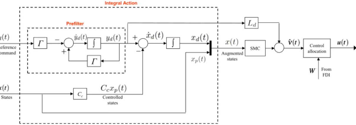
Control allocation From FDI SMC ∫ ∫ Γ Γ Reference command Prefilter Cc Controlled states States Augmented states Integral Action
Fig. 3. Integral Action Controller Structures
horizontal stabilizer deflection δs (rad), and collective EPR el. The realization in (11) and (12) is associated with
the partition in (2) and indicates the dimension of the virtual control l: specifically lt= 2 and ll= 1.
Note that in nominal conditions, true air speedVtas(m/s) is regulated using an outer loop PID controller (similar
to the altitude and heading control loops). However, in the case when all control surfaces are lost, speed is not directly regulated but assumed to vary (open loop) around its steady state trim value due to the phugoid motion.
A. Integral Action Tracking
For tracking purposes, integral action [32], [29] has been included in both the lateral and longitudinal controllers. Figure 3 gives a general overview of the integral action scheme. The idea is to obtain tracking capability of low frequency commands by augmenting the plant states xp(t) with integral action states xd(t), and then designing a
regulator scheme based on the augmented states x(t) := [xd(t)T xp(t)T]T.
The integral action statesxd(t)are obtained by integrating the ‘error’ formed by the difference between a low pass
filtered reference command signal yd(t) and the controlled states Ccxp(t) from the plant (where Cc ∈IRl×n). The
filtered reference command signal yd(t) is used instead of the actual reference command signalYd(t)to ameliorate
sudden and abrupt pilot inputs. Using the filtered reference command signal yd(t) also adds a further degree of
design freedom for controller tuning (via the choice low pass filter parameter Γ ∈IRl×l which is a stable design matrix). Note that the control law in Figure 3 also includes an additional feedforward term Ldyd(t) because of the
tracking element in the formulation.
A state-space representation of the augmented system from which the control law will be designed can be written as ˙ x(t) =Ax(t) +BW u(t) +Bdyd(t) (13) where A= [ 0 −Cc 0 Ap ] B = [ 0 Bp ] Bd= [ Il 0 ] (14) The new augmented system (A, B) is controllable if the actual system (Ap, Bp) is controllable and (Ap, Bp, Cc)
does not have any zeros at the origin (see Edwards & Spurgeon [29] for details).
B. Lateral & Longitudinal Controller Designs
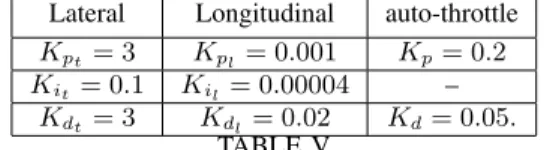
The controller design variables and gains are summarized in Table II, III, IV and V.
The sliding surface matrixS underpinning the sliding mode controller was chosen to minimize the performance measure
J =
∫ ∞
tσ
x(t)TQx(t) dt (15)
where tσ is the time at which the sliding motion is established [32], [29]. In (15) the quantity Q is a symmetric
positive definite (s.p.d) matrix used to tune the closed-loop response. The s.p.d weighting matricesQfor the lateral and longitudinal controllers are shown in Table II. The first two terms ofQt and the first term ofQl are associated
Design Variables Lateral Longitudinal Q Qt=diag(0.005,0.1,50,50,1,1) Ql=diag(0.1,2,1,1)
The integral action pre-filter matrix Γt=−0.5I2 Γl=−0.5
Sigmoidal approximation scalar δt= 0.05 δl= 0.05
Reduced order sliding poles {−0.0715,−0.1333,−0.1724±0.1354i} {−1.0351,−0.1859±0.1422i,}
TABLE II
DESIGNVALUES AND CONTROLLER GAINS
Stability analysis Lateral Longitudinal
Fault gain (22) γ0t = 4.6163 γ0l= 27.7063
Hyperplane gain (23) γ1t = 0.0050 γ1l= 0.0066
Uniqueness test (23) γ0tγ1t= 0.0232<1 γ0lγ1l= 0.1838<1
H∞ norm (25) ∥G˜t(s)∥∞=γ2t= 0.1489 ∥G˜l(s)∥∞=γ2l= 0.0024
Final stability test (26) γ2tγ0t
1−γ1tγ0t
= 0.7034<1 γ2lγ0l
1−γ1lγ0l
= 0.0816<1
TABLE III
STABILITY ANALYSIS(FOR DETAILS OF THE GAINSγ0,γ1ANDγ2SEE THE APPENDIX)
with the integral action and are less heavily weighted. The third and fourth terms of Qt and the third term of Ql
are associated with the equations of angular acceleration in roll, yaw and pitch (i.e. the Bt,2 term partition in (2))
and thus weight the virtual control. Thus by analogy to a more typical LQR framework, they affect the speed of response of the closed loop system. Here, the third and fourth terms of Qt and the third term of Ql have been
heavily weighted compared to the last two terms of Qt andQl to effect a fast closed loop system response.
The pre-filter matricesΓtandΓl from Table II (and Figure 3) have been designed to represent the ideal response
in the ϕ, β andγ channels. The scalarγ0t associated with the fault and defined formally in (22) is shown in Table
III. This has been obtained based on the assumption that, in normal operation, the ailerons and spoilers will be the primary control surfaces for ϕ tracking, whilst the differential thrust from the four engines is the associated redundancy. Similarly, γ0l has been obtained based on the assumption that in normal operation, the elevators will
be the primary control surface for flight path angle tracking, whilst the horizontal stabilizer and collective thrust introduce redundancy. The gain γ1 associated with the choice of hyperplane defined in (23) and theH∞ normγ2
associated with the reduced order sliding motion defined in (25) are both given in Table III. Simple calculations show that the stability condition from equation (26) in the appendix, expressed as 0< 1−γ2γ0γ1γ0 <1, is satisfied for both designs. This shows that the lateral and longitudinal closed loop systems are stable for all W(t)∈ W [16].
The variables related to the adaptive nonlinear gainρ(t, x)in (8) are given in Table IV. For SRS implementation, a smoothed sigmoidal approximation ∥σσ∥+δ has been used instead of the discontinuous pure unit vector term ∥σσ∥ in (7) (see for example §3.7 in [29]). The smoothed sigmoidal approximation removes chattering. In addition, the smooth approximation introduces a further degree of tuning to accommodate the actuator rate limits. This is very important especially during actuator fault or failure conditions. The scalarsδfor both the lateral (δt) and longitudinal
(δl) controller are given in Table II.
An outer loop PID heading and altitude controller used and tested in [17], has been used to provide a roll and flight path angle command to the inner–loop sliding mode controllers (lateral and longitudinal) – see Figure 5. The gains are given in Table V. Note that to eliminate steady state error, integrator components are activated when the heading angle and altitude errors are less than 5◦ and 15m respectively.
An auto-throttle for speed control has also been implemented using a PID to regulate the speed in nominal conditions (see Figure 5). These gains are available in Table V. In the event of total hydraulic failure, the outer loop PID speed control is not used (since in terms of static stability, speed control is not possible as stabilizer trim is not considered to be available in this paper). This will result in the inability of the outer-loop PID auto-throttle to maintain the commanded speed during a total loss of control surfaces, and instead, the speed will fluctuate around the commanded set-point (due to the phugoid motion – this will be seen in the simulation results). The PID gains for the lateral, longitudinal and auto-throttle have been obtained through ad-hoc tuning processes.
Note that both the lateral and longitudinal inner-loop controllers, as well as the outer-loop PID auto-throttle, manipulate the engine EPRs. For lateral control, differential engine EPR is required; whilst for longitudinal control, collective EPR is used. In the implementation, ‘control mixing’ (Figure 4) has been employed, where the EPR
Lateral Longitudinal l1t = 0, l2t = 1 l1l= 0, l2l= 1 ηt= 1 ηl= 1 ρmaxt = 2 ρmaxl= 2 at= 100, bt= 0.001 al= 100, bl= 0.001 ϵt= 1×10⁻² ϵl= 1×10⁻² TABLE IV
ADAPTIVE MODULATION GAIN VARIABLES
Lateral Longitudinal auto-throttle
Kpt = 3 Kpl= 0.001 Kp= 0.2
Kit = 0.1 Kil= 0.00004 –
Kdt = 3 Kdl= 0.02 Kd= 0.05.
TABLE V
OUTER LOOP HEADING,ALTITUDE AND SPEEDPIDGAINS
+ + + + + + Lead Compensator 1 Lead Compensator 2 Lead Compensator 3 To Engine 1 To Engine 2 To Engine 3 + + b b b e1t e2t +
+ Compensator 4Lead To Engine 4
b e3t e4t el eVtas e1 e2 e3 e4 OUTPUTS EPR ‘Control Mixing’ INPUTS: EPR signals from controller Lateral differential EPR Longitudinal collective EPR auto throttle outer-loop PID collective EPR
Fig. 4. EPR ‘control mixing’
signals from both the lateral controller (e1t, e2t, e3t and e4t), the longitudinal controller (el) and outer-loop PID
speed control EPR (eVtas), are added together before being applied to each of the engines. This is similar to the
control strategy used for the NASA propulsion control aircraft [6]. Note in Figure 4 the presence of phase advance compensators. These have been introduced to compensate for the un-modelled engine dynamics which results in a lag between the commanded EPR and the generation of thrust. This lag is compensated for by the phase-advance structure, to improve performance.
In the SRS implementation, an ILS scenario has been used to create roll and flight path angle demands for the inner loop sliding mode controller. This provides an automatic landing feature obviating the need for pilot commands. Details of the ILS landing scheme can be found in [17].
Remark:Although some control features (such as the outer loop PID heading, altitude and ILS landing capability)
have been taken from previous tests [17], the inner core sliding mode controller is new. The previous controllers were designed with no consideration of a situation in which all control surfaces are lost. The new controller has wider tolerance to different types of actuator faults/failures especially and specifically the loss of all hydraulic systems. The overall controller interconnections are given in Figure 5.
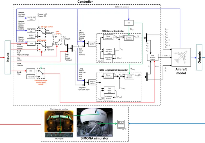
V. SRSIMPLEMENTATION ISSUES
The aircraft model running the SRS 6-DOF flight simulator, is a high fidelity nonlinear model of a civil aircraft based on the RECOVER benchmark model from the GARTEUR FM-AG16 programme [33]. For these tests the RECOVER model has been modified to include a total loss of all control surfaces scenario, which was not considered in the GARTEUR FM-AG16 programme.
The control scheme was converted from SIMULINK blocks into C-code using the Real Time Workshop with its inputs/outputs appropriately ordered to integrate with the SRS facility as shown in Figure 5. The controller was implemented based on a fixed integration time step of 0.01s – which corresponds to the specified sensor update rates of 100Hz (current industrial practice).
The computational load, measured as the time needed for a single integration step on the flight computer, was found to be 0.15ms. The available processing power is sufficient to run the controller in real-time, i.e. within a 10 ms time frame. This is made possible by keeping the design as simple as possible, while at the same time ensuring the stability and performance during faults and failures. The combination of sliding modes and control allocation contributes to the simple robust design. Here, the control allocation aspect allows the scheme to handle various
ulat(t) Cmd: Roll Sideslip Flight path Pilot switch PID Cmd: Roll Flight path angle Cmd: Heading Altitude Cmd: Sideslip Roll Flight path MCP switch
States x(t) & sensors
Roll=0 FPA=0 LOC & GS
PID RollFlight path APP switch Roll Flight path LOC & GS logic Aircraft Controller
ILS logic switch
Control allocation νlat(t) Linear component νllat νnlat Adaptive unit vector term SMC lateral Controller SMC longitudinal Controller Lat cmd: Roll Sideslip Lat states: Roll rate Yaw rate Sideslip Roll Long Engage LOC Engage GS Sensor: LOC valid GS valid Sensor: LOC dev GS dev States: heading States: Heading Altitude δair δail δaor δaol δsp-1-4 δsp5 δsp9-12 δr δe δ e1t e2t e3t e4t el e1 e2 e3 e4 In p u ts O u tp u ts Integral Action FDI Wlat Wlong EPR Control mixing evtas Adaptation scheme ||σlat|| ρlat(t) Aircraft model Control allocation νlong(t) Linear component νllong νnlong Unit vector term SMC longitudinal Controller ulong(t) Long cmd: Flight path angle
Long states: Pitch rate Vtas AoA pitch e δs MCP inputs Pilot inputs and switches
SIMONA simulator Data logging Integral Action Cmd: Vtas PID Wlong
Flight path angle priority logic switch Vtas hold ρlong(t) Adaptation scheme ||σlong||
Fig. 5. Controller interconnections
types of actuator faults and failures without restructuring or reconfiguring the controller itself. Instead, the signal from the sliding mode controller is simply redistributed to the remaining ‘healthy’ control surfaces, which in this case are the engines.
The RECOVER benchmark model was modified in order to include the new failure condition which represents the total loss of hydraulics. The total loss of all control surfaces has been implemented as a control surface jam and lock-in-place at a particular time during straight and level flight (jammed at trim control surface deflection). This replicates the ineffectiveness of the control surfaces to provide commanded moments due to the loss of hydraulics. It is assumed that no control surfaces float, but instead, lock in place due to mechanical resistance.
The engines have been modeled using data obtained from NASA [22] which includes engine transient charac-teristics through tests on the Pratt & Whitney JT9D turbofan. The engine model comprises linear dynamics and a nonlinear look-up table tailored to capture the data from [23], [22]. The overall nonlinear model produces first-order-like lag behaviour between the EPR command (the control input) and the thrust output. All the other control surfaces are modeled with realistic position limits and rate limits with data from NASA [23], [22].
The results in the next section represent proof of concept and show a successful real time implementation of the proposed controller.
VI. SIMONA SIMULATOREVALUATIONRESULTS
The results presented in this section have been obtained from the data logging features on the SRS during the evaluation tests. It is assumed that measurements of the actual actuator deflections are available, which is common in passenger aircraft [1]. This information is used to calculate W for the control allocation scheme.
As in the GARTEUR FM-AG16 benchmark problem, it will be assumed that the aircraft is in a low speed configuration (a mass of 263000kg, speed of 92.6m/s, altitude of 600m and flap angle of 20◦). For comparison, the flight manoeuvre used in the tests is also similar to the GARTEUR FM-AG16 benchmark problem [33], [34],
[17]. Shortly after a right turn, the complete loss of all control surfaces occurs and all the control surfaces become inactive with flaps locked at 20◦ extension. The required action is to manoeuvre the aircraft and to achieve a safe emergency landing.
Here, a low speed configuration with a 20◦ flap extension was considered, which is close to an extreme point in the flight envelope (as Vtas is very close to the stall speed [22]). Most of the NASA PCA tests on the B747
aircraft were conducted on a B747 aircraft with flaps up (0◦ extension) but at a higher speed [6], [7] (and possibly lighter weight). The reason this configuration is not considered in this paper, is to allow direct comparisons of the controller performance – albeit on a different fault and failure condition – to the controllers tested on the GARTEUR FM-AG16 benchmark problem [21], [17]. Furthermore, in a B747 aircraft, the trailing edge flaps, although normally driven by hydraulics, are also driven by electric motors in case of hydraulic failure [22], [6]. Note that the flight test condition is slightly different to the design trim. This adds realism and further ‘challenges’ the robustness of the controller. Note that during the SRS evaluation tests, no wind and gust effects are considered.
Figure 6(a) illustrates the overall flight manoeuvre. The simulation starts under the hypothesis that the aircraft is in straight and level flight heading north (0◦) with low speed flight conditions mentioned above. This is followed by a 90◦ right turn heading east (90◦). After the aircraft has stabilized from the turn, the loss of hydraulics occurs at 228s. Realizing that conventional control does not work, an altitude change to 2500ft and then back to 2000ft was conducted to test the climb and descent capabilities of the aircraft using engines only. Then another 90◦ right turn is attempted, changing heading to south (180◦). Finally a small right turn changing heading to 240◦ was carried out in order to intercept the ILS signals from Runway 27 at a heading of 269◦. At this stage, the approach button (APP button) on the mode control panel (MCP) is activated to arm the ILS signal capture. When the LOC signal becomes valid (at 484s), the LOC PID control is engaged (Figure 7(b)). This allows the aircraft to be lined up with the runway. Then, when the GS signal becomes valid (at 645s), the GS PID controller is engaged (Figure 7(b)) providing descent guidance to the runway (at 3◦ flight path angles). The flare and the actual landing of the aircraft are not attempted and the simulation was stopped 50m above ground level.
Figures 6(a)-7 show the flight trajectory of the controller under nominal no-fault conditions and in the hydraulic loss scenario. It can be seen from the comparisons between the nominal no-fault trajectory and the propulsion controlled trajectory, that there is almost no difference in performance. The slight difference is in part due to the different timings of when the manoeuvres take place because of the pilot in the loop, and not because of performance degradation. The LOC and GS approach shows virtually no difference between the nominal no-fault condition and the propulsion controlled case.
Figure 7(b) shows the ILS signals for both the nominal and propulsion controlled cases. The distance measurement equipment (DME) signal indicates how far the aircraft is from the runway. This distance is used for LOC and GS valid range measurements. The LOC deviation gives the error between the centerline of the runway and the aircraft lateral distance. The GS deviation represents the deviation from the desired -3◦ descent trajectory to the runway.
Figure 7(a) is an alternative view to Figure 6(a) and shows the aircraft’s earth position with time. Again this figure shows that nominal performance is maintained during the failure case.
A. Nominal Condition
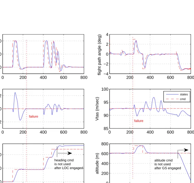
Figures 8-10 show the results obtained from the nominal no-fault flight condition tests. Figure 8 shows the controlled states. The heading and roll plots show the three 90◦ right turns undertaken to return to Runway 27 before the LOC is engaged and the heading lines-up with the runway. The altitude and flight path angle plots show that during the roll manoeuvre, the altitude was maintained at 600m (approx 2000ft). Good tracking is also observed when the altitude was increased to 762m (2500ft) and returned back to 600m. When the GS is engaged, good flight path angle tracking at -3◦ can be observed. Note that the roll demand is limited to 20◦.
The sideslip command is set to 0◦ while the PID auto-throttle is set to maintain speed at 92.6m/s (180kts). Note that when the LOC and GS are engaged (at 484s and 645s respectively), the heading and altitude commands from the MCP are not used. Instead, the inner-loop roll and flight path angle command are provided by the ILS PID outer-loop controller, which guides the aircraft to line-up with the runway and touchdown on the target zone.
Figure 9 shows the nominal control surface deflections during the manoeuvres. Note that the spoilers and stabilizers were also used during the test due to the control allocation structure of the controller. Finally Figure 10 shows the variation in the norm of the switching function signals for both the lateral and longitudinal controller in the fault-free condition.
roll angle side slip angle heading flight path angle speed altitude
Nominal 4.1695 0.8520 27.4632 0.5546 0.1677 37.3875
PCA 4.2271 0.5678 27.2218 0.5095 1.5856 37.3443
Difference 0.0576 -0.2842 -0.2412 -0.0451 1.4179 -0.0432
TABLE VI
RMSVALUES FOR STATES TRACKING ERROR
B. Propulsion controlled
Figures 11-13 show the results obtained from a test involving the loss of all control surfaces. At 228s, the failure occurs and only the engines are available for manipulation.
Despite losing all the control surfaces, the propulsion controlled aircraft still manages to maintain the nominal heading and altitude tracking as shown in Figure 11. Note that in the event of total loss of the control surfaces, the speed remains close to the trim speed with a deviation smaller than ±7m/s. This deviation in speed from its trim is expected and can also be seen in most of the NASA results [6], [7].
Using only engine control, outer-loop heading and altitude control is still possible as shown in Figure 11. This is also seen by the good tracking of the inner-loop roll and flight path angle commands. As in the nominal fault-free test, sideslip remains close to zero. Compared to the nominal fault-free condition, the ILS landing performance of the propulsion controlled aircraft shows no visible degradation (see also Figures 6(a)-7).
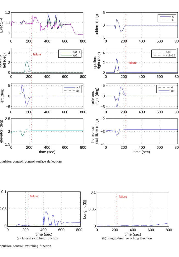
Figure 12 clearly shows the effect of losing all control surfaces. Before the failure occurs, all the control surfaces are active but after the failure, all the control surfaces are locked in place. Once the failure occurs, the control allocation property of the proposed scheme is used to redistribute the control signals to the remaining ‘control surfaces’ (i.e. the engines) using the effectiveness level of the actuators. Once the failure occurs, the EPR signals in Figure 12 are different to the nominal ones in Figure 9. This is due to the redistribution of the control signals from all the usual control surfaces to the engines (through EPR). The most visible difference is during the altitude change tests and during the roll manoeuvres where the differential thrust is more visible.
Figure 14 shows the 4 EPR signals from Figure 12 in detail. Here, it is clear how the EPR (and therefore engine thrust) is used for roll and flight path angle control. Immediately after the failure, an increase in altitude to 762m (2500ft) was commanded to test the climb capability of the aircraft. As seen in the altitude plot in Figure 11, this is achieved without performance degradation compared to the nominal altitude tracking in Figure 8. During this altitude change test, it can be seen in Figure 14 that collective thrust was used to achieve the desired flight path angle – as discussed in Section II. Also, as discussed in Section II, during the roll manoeuvres, differential thrust is used. This can also be seen in Figure 14. Finally, when the GS is engaged, the collective thrust is again used for flight path angle control and descent towards the touchdown target zone.
Remark:Note that in Figure 14 four different EPR signals are present. However during a longitudinal manoeuvre
e.g. a change of altitude, all the EPR signals have (visually at least) the same value and therefore all four lines overlap on top of each other in the plots. Typically the four separate EPR signals will only be visible when there is differential thrust between engines 1 and 2 (on the left wing) and engines 3 and 4 (on the right wing) in order to perform lateral manoeuvres e.g. a change in roll angle.
Figure 13 shows small deviations of the switching function signals (compared to the nominal ones in Figure 10) after the failure occurs. The deviation of the switching function from its nominal condition indicates the level of difficulty, and the extra effort the sliding mode controller needs apply to maintain the desired performance.
Table VI shows the root mean square (RMS) values for the state tracking errors in both the nominal and propulsion controlled cases. This table shows similar RMS values for the states tracking error in both nominal and PCA conditions, indicating that the proposed PCA scheme has managed to retain close to the nominal tracking performance. The exception is speed tracking, because in the PCA case there is no direct speed control due to the lack of redundancy (recall that in this paper, stabilizer trim is not considered to be available when total control surface failure occurs).
1) Performance analysis during altitude increase: Figure 15 shows a detailed analysis of the controlled states
and the EPR signals during the altitude change (the 230 sec-319 sec time interval) for both the nominal and failure case. Figure 15(a) shows the altitude tracking performance and shows that after the failure occurs, nominal altitude tracking performance is still maintained despite using only engines. This figure shows a damped altitude tracking with a rise time of 88 sec and no oscillatory mode visible with no overshoot and no steady state error
for both the nominal and failure cases. The slight difference between the nominal and failure case is not due to tracking performance degradation, but due to the small change in speed (note that speed is not tracked during the failure case to give priority to flight path angle tracking). Figure 15(b) shows the collective EPR signals during the altitude increase. Here, small oscillations during the start of the manoeuvre can be observed, to damp the aircraft longitudinal oscillatory modes, but they quickly disappear.
Remark: Note that there are small oscillations in Figure 15(b) which are present before the change in altitude
command (at 231 sec). These underdamped oscillation are transients which arise from the loss of all the control surfaces at 228 sec. The appearance of the oscillations corresponds exactly with the time when the signals from the controller begin to be totally re-routed to the engines.
2) Performance analysis during heading change: Figure 16 shows a detailed analysis of the controlled states
and the EPR signals during the heading change (the 397 sec-481 sec time interval) for both the nominal and failure case. As before, Figure 16(a) shows that the nominal heading performance is still maintained in the failure case with a rise time of 64 sec, with well damped heading tracking and negligible tracking error. Again, the differences in heading are due to changes in speed for the failure case. Figure 16(b) clearly shows the differential EPR signals during the heading change. The small oscillations visible at the start of the heading change, quickly disappear, this time to damp the aircraft lateral oscillatory modes.
3) Performance analysis compared to previous GARTEUR FM-AG16 results: The results in Figures 15-16
specifically, and Figures 6(a)-12 in general, show that, despite losing all the control surfaces, the proposed sliding mode control allocation scheme manages to maintain the same level of guidance/control characteristic with almost no degradation when using only engines. This post failure capability of maintaining nominal guidance/control characteristic matches the previous GARTEUR FM-AG16 results [21], [17].
VII. CONCLUSIONS
This paper has described the implementation of a sliding mode control allocation scheme on the 6-DOF SIMONA Research Simulator. The results represent realistic flight manoeuvres, designed to test the capabilities and the performance of the controller in nominal fault-free conditions, and during a propulsion only control emergency situation. During the failure conditions, the same controller (designed for the nominal fault-free case) is also used for propulsion control without controller reconfiguration. This is achieved through automatic redistribution of the control signals to the engines based on knowledge of the ‘health’ of the actuators. The results from the simulator tests show only small differences between the performance of the propulsion controlled aircraft and the nominal case. With the exception of speed, which is not directly regulated when all control surfaces are lost, the difference in the state tracking error RMS values between the propulsion controlled aircraft and the nominal case is less than 1%. Furthermore the performance of the propulsion controlled aircraft during the altitude increase and heading change manoeuvres shows almost no degradation at all. It must be stressed that these results have been achieved using a relatively simple controller designed about a single trim condition, and comprising a fixed linear feedback gain and a nonlinear term with a simple scalar adaptive modulation gain. This controller has been shown to retain good performance, even in the presence of faults, in a region of the flight envelope well away from the trim condition. Future work seeks to extend these ideas into an linear parameter varying framework to widen (theoretically) the controller’s region of applicability, and then to rigorously test its performance throughout the flight envelope based on worst case scenarios.
REFERENCES
[1] D. Bri`ere, P. Traverse, Airbus A320/A330/A340 electrical flight controls: A family of fault-tolerant systems., Digest of Papers FTCS-23 The Twenty-Third International Symposium on Fault-Tolerant Computing (1993) 616–623.
[2] M. Job, Air Disaster: Volume 2, Aerospace Publications Pty Ltd, 1996.
[3] F. W. Burcham, C. G. Fullertron, T. A. Maine, Manual manipulaton of engine throttles for emergency flight control, Tech. Rep. NASA/TM-2004-212045, NASA (2004).
[4] D. Learmount, Great escape, Flight International.
[5] B. Lemaignan, Flying with no flight controls: Handling qualities analyses of the baghdad event, in: AIAA Atmospheric Flight Mechanics Conference and Exhibit, no. AIAA 2005-5907, 2005.
[6] F. W. Burcham, T. A. Maine, J. Kaneshinge, J. Bull, Simulator evaluation of simplified propulsion–only emergency flight control system on transport aircraft, Tech. Rep. NASA/TM-1999-206578, NASA (1999).
[7] F. W. Burcham, T. A. Maine, J. Burken, J. Bull, Using engine thrust for emergency flight control: MD–11 and B–747 results, Technical Memorandum NASA/TM–1998–206552, NASA (1998).
[8] F. W. Burcham, J. Burken, T. A. Maine, J. Bull, Emergency flight control using only engine thrust and lateral center-of-gravity offset: A first look, Technical Memorandum NASA/TM-4789, NASA (1997).
[9] F. Burcham, J. Burken, T. A. Maine, Flight testing a propulsion-controlled aircraft emergency flight control system on a F-15 airplane, in: AIAA Biennial Flight Test Conference, no. AIAA 94-2123-CP, 1994.
[10] F. W. Burcham, C. G. Fullerton, Controlling crippled aircraft – with throttles, Technical Meomrandum 104238, NASA (1991). [11] E. A. Jonckheere, G. R. Yu, C. C. Chien, Gain Scheduling for Lateral Motion of Propulsion Controlled Aircraft Using Neural Networks,
in: American Control Conference, 1997, pp. 3321–3325.
[12] Y. Ochi, Flight control system design for propulsion–controlled aircraft, Proc. Institution of Mechanical Engineers, Part G:J. Aerospace Engineering 219 (2005) 329–340.
[13] M. Harefors, D. G. Bates, Integrated propulsion-based flight control system design for a civil transport aircraft, International Journal of Turbo and Jet Engines 20 (2003) 95–114.
[14] J. Fuller, Integrated flight and propulsion control for loss-of-control prevention, in: AIAA Guidance, Navigation and Control Conference and Exhibit, no. AIAA-2012-4896, 2012.
[15] C. Edwards, T. Lombaerts, H. Smaili, (Eds.), Fault Tolerant Flight Control: A Benchmark Challenge, Vol. 399, Springer-Verlag: Lecture Notes in Control and Information Sciences, 2010.
[16] H. Alwi, C. Edwards, Fault tolerant control using sliding modes with on-line control allocation, Automatica 44 (7) (2008) 1859–1866. [17] H. Alwi, C. Edwards, O. Stroosma, J. A. Mulder, Evaluation of a sliding mode fault-tolerant controller for the El Al incident, AIAA
journal of Guidance Control and Dynamics 33 (3) (2010) 677–694.
[18] D. Shin, G. Moon, Y. Kim, Design of reconfigurable flight control system using adaptive sliding mode control: actuator fault, Proceedings of the Institution of Mechanical Engineers, Part G (Journal of Aerospace Engineering) 219 (4) (2005) 321–328.
[19] S. R. Wells, R. A. Hess, Multi–input/multi–output sliding mode control for a tailless fighter aircraft, Journal of Guidance, Control and Dynamics 26 (3) (2003) 463–473.
[20] Y. Shtessel, J. Buffington, S. Banda, Tailless aircraft flight control using multiple time scale re-configurable sliding modes, IEEE Transactions on Control Systems Technology 10 (2) (2002) 288–296.
[21] H. Alwi, C. Edwards, O. Stroosma, J. A. Mulder, Fault tolerant sliding mode control design with piloted simulator evaluation, AIAA Journal of Guidance, Control and Dynamics 31 (5) (2008) 1186–1201.
[22] C. Hanke, D. Nordwall, The simulation of a jumbo jet transport aircraft. Volume II: Modelling data, Tech. Rep. CR-114494/D6-30643-VOL2, NASA and The Boeing Company (1970).
[23] C. Hanke, The simulation of a large jet transport aircraft. Volume I: Mathematical model, Tech. Rep. CR-1756, NASA and the Boeing company (1971).
[24] M. Cook, Flight Dynamics Principles, Second Edition: A Linear Systems Approach to Aircraft Stability and Control, Butterworth-Heinemann, 2007.
[25] M. Hamayun, C. Edwards, H. Alwi, A fault tolerant control allocation scheme with output integral sliding modes, Automatica 49 (2013) 1830–1837.
[26] C. P. Tan, C. Edwards, Sliding mode observers for robust detection and reconstruction of actuator and sensor faults, International Journal of Robust and Nonlinear Control 13 (2003) 443–463.
[27] Y. M. Zhang, J. Jiang, Active fault-tolerant control system against partial actuator failures, IEE Proceedings: Control Theory & Applications 149 (2002) 95–104.
[28] O. H¨arkeg˚ard, S. T. Glad, Resolving actuator redundancy - optimal control vs. control allocation, Automatica 41 (1) (2005) 137–144. [29] C. Edwards, S. K. Spurgeon, Sliding Mode Control: Theory and Applications, Taylor & Francis, 1998.
[30] Y. Shtessel, C. Edwards, L. Fridman, A. Levant, Sliding Mode Control and Observation, Birkhauser, 2013.
[31] F. Plestan, Y. Shtessel, V. Bregeault, A. Poznyak, New methodologies for adaptive sliding mode control, International Journal of Control 83 (9) (2010) 1907–1919.
[32] V. I. Utkin, Sliding Modes in Control Optimization, Springer-Verlag, Berlin, 1992.
[33] H. Smaili, J. Breeman, T. Lombaerts, D. Joosten, Recover: A benchmark for integrated fault tolerant flight control evaluation, in: C. Edwards, T. Lombaerts, H. Smaili (Eds.), Fault Tolerant Flight Control, Vol. 399 of Lecture Notes in Control and Information Sciences, Springer Berlin / Heidelberg, 2010, pp. 171–221.
[34] O. Stroosma, T. Lombaerts, H. Smaili, M. Mulder, Real-time assessment and piloted evaluation of fault tolerant flight control designs in the SIMONA research flight simulator, in: C. Edwards, T. Lombaerts, H. Smaili (Eds.), Fault Tolerant Flight Control, Vol. 399 of Lecture Notes in Control and Information Sciences, Springer Berlin / Heidelberg, 2010, pp. 500–517.
APPENDIX A: CONTROLLERDESIGNPROCEDURE
The proposed controller design procedure from [21], [16], to synthesize the design matrix S (and consequently the virtual controller νˆ(t) from (4)) can be expressed as follows:
1) Re–order the states and partition the input distribution matrix B as in (2) to obtain B1 and B2. Then scale
the states of the system in (1) so that B2B2T =Il. This can be achieved without loss of generality. Define
BN2 := (I−B2TB2) (16)
then by construction B2NB2T = 0 since B2NB2T =B2T−B2T(| {z }B2BT2) I
2) Change coordinates using the linear transformation x(t)7→xˆ(t) =Trx(t) where Tr:= [ I −B1B2T 0 I ] (17) It is shown in [16] in the new coordinates that the system in (1) can be written as
[ ˙ˆ x1(t) ˙ˆ x2(t) ] | {z } ˙ˆ x(t) = [ ˆ A11 Aˆ12 ˆ A21 Aˆ22 ] | {z } ˆ A=TrATr [ ˆ x1(t) ˆ x2(t) ] | {z } ˆ x(t) + [ 0 I ] | {z } ˆ B=TrB ˆ ν(t) + [ B1B2NB2+ 0 ] ˆ ν(t) (18) where B+2 :=W2BT2(B2W2BT2)−1 (19)
In (18), the state partition xˆ1∈IR(n−l) andxˆ2∈IRl and νˆ(t)∈IRl is the virtual control.
3) Define a switching functionσ(t) : IRn→IRlto beσ(t) =Sx(t)whereS∈IRl×nand by choicedet(SBν) = Il. In the xˆ(t) coordinates in (18), a suitable choice for the sliding surface is
ˆ S:=STr−1= [ M Il ] (20) where M ∈IRl×(n−l) represents design freedom. The matrix M from (20) must be chosen so that, A˜11:=
ˆ
A11−Aˆ12M is stable and Aˆ11 and Aˆ12 are defined in (18). If ( ˆA,Bˆ) is controllable (or equivalently if (A, BB2T) is controllable), then ( ˆA11,Aˆ12) is controllable [29], and such a matrix M can always be found.
Note from (20), that in the original coordinates
S=[ M I ]Tr=
[
M I−M B1B2T ]
(21) 4) To satisfy the stability analysis requirements and guarantee closed loop stability for allW ∈ W in (5):
a) Calculate the smallest γ0 such that
∥W2B2T(B2W B2T)−1∥< γ0 (22)
for all W ∈ W. A finite bound γ0 is guaranteed to exist [16].
b) Check
γ1:=∥M B1B2N∥< 1
γ0
(23) where γ0 is given in (22) and B2N is given in (16). If (23) is not satisfied, it is necessary to re-design
the matrix M. c) Define
˜
G(s) := ˜A21(sI−A˜11)−1B1B2N (24)
where the matrix A˜21:=MA˜11+ ˆA21−Aˆ22 andA˜11:= ˆA11−Aˆ12M. By construction,G˜(s) is stable
and define
γ2 =∥G˜(s)∥∞ (25)
d) Ifγ2 < γ01 −γ1, then as shown in [16] the closed loop is stable for all W ∈ W.
Note that the inequalities in 4(b) and 4(c) above can be conveniently combined to give a compact single constraint 0< γ2γ0
1−γ1γ0
<1 (26)
0 2000 4000 6000 8000 10000 12000 14000 0 0.5 1 1.5 2 2.5 3 x 10⁴ 0 100 200 300 400 500 600 700 800 ye xe he nominal propulsion controlled right turn LOC intercept S loss of all hydraulic start end GS intercept altitude increase altitude decrease right turn right turn straight & level flight N W E X (a) 3-D view Fig. 6. SRS flight trajectory of the nominal and PCA aircraft.
0 100 200 300 400 500 600 700 800 0 200 400 600 800 he 0 100 200 300 400 500 600 700 800 0 5000 10000 15000 xe 0 100 200 300 400 500 600 700 800 0 1 2 3x 10 4 time (sec) ye nominal propulsion controlled LOC intercept GS intercept failure
(a) aircraft earth position with time
0 100 200 300 400 500 600 700 800 0 1 2 3 4x 10 4 DME (m) 0 100 200 300 400 500 600 700 800 −8 −6 −4 −2 0 2
LOC deviation (deg)
0 100 200 300 400 500 600 700 800 −0.5 0 0.5 1 GS deviation (deg) time (sec) nominal propulsion controlled LOC valid GS valid X GS engaged X LOC engaged failure X (b) ILS signals Fig. 7. aircraft earth position and ILS signals of the nominal and PCA aircraft.
0 200 400 600 800 −2
0 2
side slip angle (deg)
0 200 400 600 800
0 10 20
roll angle (deg)
0 200 400 600 800
0 100 200
heading angle (deg)
time (sec) 0 200 400 600 800 91.5 92 92.5 93 93.5 Vtas (m/sec) 0 200 400 600 800 0 200 400 600 800 altitude (m) time (sec) 0 200 400 600 800 −2 0 2
flight path angle (deg)
states cmd
altitude cmd is not used after GS engaged heading cmd is not used
after LOC engaged
0 200 400 600 800 1 1.1 1.2 EPR 1−4 0 200 400 600 800 0 2 4
spoilers left (deg)
sp1−4 sp5 0 200 400 600 800 0 2 4
spoilers right (deg)
sp8 sp9−12 0 200 400 600 800 −5 0 5
ailerons left (deg)
aol ail 0 200 400 600 800 −5 0 5
ailerons right (deg) air
aor 0 200 400 600 800 −5 0 5 rudders (deg) ru rl 0 200 400 600 800 1.5 2 2.5 elevator (deg) time (sec) 0 200 400 600 800 −4 −3 −2 horizontal stabilizer (deg) time (sec) Fig. 9. nominal condition: control surface
0 200 400 600 800 0 0.05 0.1 Lat || σ (t)|| time (sec) (a) lateral switching function
0 200 400 600 800 0 0.05 0.1 Long || σ (t)|| time (sec) (b) longitudinal switching function Fig. 10. nominal condition: switching function
0 200 400 600 800 −2
0 2
side slip angle (deg)
0 200 400 600 800
0 10 20
roll angle (deg)
0 200 400 600 800
0 100 200
heading angle (deg)
time (sec) 0 200 400 600 800 85 90 95 100 Vtas (m/sec) 0 200 400 600 800 0 200 400 600 800 altitude (m) time (sec) 0 200 400 600 800 −4 −2 0 2 4
flight path angle (deg)
states cmd altitude cmd is not used after GS engaged heading cmd is not used after LOC engaged
failure failure
0 200 400 600 800 1 1.1 1.2 EPR 1−4 0 200 400 600 800 0 2 4
spoilers left (deg)
sp1−4 sp5 0 200 400 600 800 0 2 4
spoilers right (deg)
sp8 sp9−12 0 200 400 600 800 −5 0 5
ailerons left (deg)
aol ail 0 200 400 600 800 −5 0 5
ailerons right (deg)
air aor 0 200 400 600 800 −5 0 5 rudders (deg) ru rl 0 200 400 600 800 1.5 2 2.5 elevator (deg) time (sec) 0 200 400 600 800 −4 −3 −2
horizontal stabilizer (deg)
time (sec) failure
failure
Fig. 12. propulsion control: control surface deflections
0 200 400 600 800 0 0.05 0.1 Lat || σ (t)|| time (sec) failure
(a) lateral switching function
0 200 400 600 800 0 0.05 0.1 Long || σ (t)|| time (sec) failure
(b) longitudinal switching function Fig. 13. propulsion control: switching function
0 100 200 300 400 500 600 700 800 0.95 1 1.05 1.1 1.15 1.2 time (sec) EPR EPR 1 EPR 2 EPR 3 EPR 4 EPR1,2,3,4 LOC engaged GS engaged failure roll manoeuvres roll manoeuvre straight & level flight altitude change tests
Fig. 14. propulsion control: engines pressure ratio
230 240 250 260 270 280 290 300 310 620 640 660 680 700 720 740 760 altitude (m) time (sec) nominal propulsion controlled alt cmd (a) altitude 230 240 250 260 270 280 290 300 310 1.08 1.1 1.12 1.14 1.16 1.18 1.2 1.22 time (sec) EPR EPR 1 nom EPR 2 nom EPR 3 nom EPR 4 nom EPR 1 PCA EPR 2 PCA EPR 3 PCA EPR 4 PCA
(b) oscillatory mode damping Fig. 15. Nominal Vs. propulsion control: performances during altitude increase
400 410 420 430 440 450 460 470 480 100 120 140 160 180
heading angle (deg)
time (sec) nominal propulsion controlled hdg cmd (a) heading 400 410 420 430 440 450 460 470 480 1 1.05 1.1 1.15 1.2 1.25 time (sec) EPR EPR 1 nom EPR 2 nom EPR 3 nom EPR 4 nom EPR 1 PCA EPR 2 PCA EPR 3 PCA EPR 4 PCA
(b) oscillatory mode damping Fig. 16. Nominal Vs. propulsion control: performances during heading change
![Fig. 2. Principles of throttles-only flight control (Figures adapted from [22], [23])](https://thumb-us.123doks.com/thumbv2/123dok_us/9224164.2806760/3.918.269.648.634.1072/fig-principles-throttles-flight-control-figures-adapted.webp)