Mining the relation and implication of user generated content in social media

(1)

c

(2)

MINING THE RELATION AND IMPLICATION OF USER GENERATED CONTENT IN SOCIAL MEDIA

BY XIN JIN

DISSERTATION

Submitted in partial fulfillment of the requirements for the degree of Doctor of Philosophy in Computer Science

in the Graduate College of the

University of Illinois at Urbana-Champaign, 2012

Urbana, Illinois

Doctoral Committee:

Professor Jiawei Han, Chair Professor Tarek Abdelzaher

Associate Professor Chengxiang Zhai Dr. Jie Yu, GE Global Research Center

(3)

Abstract

The phenomenal success of social media sites, such as Facebook, Twitter, LinkedIn, Flickr and YouTube, not only revolutionized the way people communicate and think, but also revolutionized the way how corporations do business. During the current age of social media, web usage can be characterized as the decentralization of online information, which now largely consists of high volume and real-time content generated from the bottom-up, where common users are the contributors and producers of information. The transition from Web 1.0 (represented by static webpages instead of dynamic user-generated content) to Web 2.0 (represented by Social Media which consists of large scale of real-time and dynamic user-generated content), makes Internet information become in larger scale, richer, more interactive and complex.

The goal of this thesis is to mine the relation and implication of user generated content in social media. In this thesis, I will present several studies that I have conducted on how to analyze such relation and implication. First, we proposed an approach for similarity computation based on both visual content and link information in social media by a novel way of mutual reinforcement of content similarity and link similarity. Second, we proposed a GAD (General Activity Detection) framework to fully explore the power of activity detection for clustering, which can be used to partition similar content objects into groups. The algorithms (both exact and approximate) developed within this framework can perform fast clustering for large scale content data. Social media content not only relate to each other, but also to outside phenomena and show strong implication with prediction power. In my third work, by aggregating user content information in social

(4)

media, we developed a unified model to integrate clustering, ranking and regression for the prediction of stock price change.

(5)

(6)

Acknowledgments

I would like to thank all the people who have supported and helped me during my Ph.D. study here at UIUC in the past five years.

I would like to express my deepest gratitude to my advisor Professor Jiawei Han for his great support and advise for my Ph.D. study. His vision, enthusiasm, and encouragement inspire me to think more solid and do interesting work. This thesis would not have been possible without his support.

Also I would like to thank other doctoral committee members, Prof. Tarek Abdelzaher, Prof. Chengxiang Zhai and Dr. Jie Yu, for their invaluable help and constructive comments on this thesis.

During my Ph.D. study, it is my great honor to work with talented researchers. I owe sincere gratitude to my collaborators and colleagues, including (but not limited to), Jiebo Luo, Liangliang Cao, Chi Wang, Scott Spangler, Sangkyum Kim, Xide Lin, Hongning Wang, Bolin Ding, Jing Gao, Zhijun Yin, Xiao Yu, Qi He, Quanquan Gu, Manish Gupta, Yizhou Sun, Cuiping Li, Jie Yu, Gang Wang, Andrew Gallagher, Dhiraj Joshi, Ying Chen, Keke Cai, Rui Ma, Mohammad Maifi Hasan Khan, Chandrasekar Ramachandran, Rahul Malik, Yintao Yu, Tianyi Wu, Tim Weninger, Thomas S. Huang, Cedar Pan, Xianyang Zhang, Zhenhui Li, LuAn Tang and Hongbo Deng.

Last but not least, I would like to thank my family for their care and support all the time.

(7)

List of Tables

3.1 Major notations. . . 12

3.2 Complexity of algorithms inHomogeneous Network. . . 14

3.3 Complexity of algorithms in (weighted)Heterogeneous Network. . . 17

3.4 Complexity of Two-Stage and IWSL inHeterogeneous Network. . . 26

3.5 Statistics for the datasets . . . 27

3.6 Top 10 most frequent tags. . . 28

4.1 Characteristics of Approximate GAD algorithms . . . 54

4.2 Basic algorithms within the GAD framework . . . 55

4.3 Statistics for datasets used in experiments . . . 63

4.4 Performance of H-GAD compared with HKM . . . 74

4.5 Performance of KD-GAD compared with kd-tree K-Means . . . 74

5.1 Notation Summarization . . . 91

5.2 Top topic clusters with top ranked topic terms. . . 107

5.3 Top ranked users. The description is extracted from the public user pro-file information on Twitter in June 2012. Note that the copyright of each description belongs to the corresponding Twitter user. . . 108

(10)

List of Figures

3.1 Information network for Flickr, connected by images, user tags and groups. 10 3.2 Information network for Amazon, connected by products, user tags and

categories. . . 10 3.3 Images with high visual similarity, but low semantic similarity. . . 19 3.4 Images annotated by the tag ”flower”, but with low visual similarity. . . 20 3.5 Tag frequency for the Flickr dataset. Y-axis denotes the frequency, X-axis

denotes the ordered (by frequency) tag id. . . 27 3.6 Tag frequency for the Amazon dataset. Y-axis denotes the frequency, X-axis

denotes the ordered (by frequency) tag id. . . 28 3.7 Speed-up of HK-SimRank and HMok-SimRank over HSimRank. X-axis

denotes the number of images, Y-axis denotes the speed-up (in times ratio). 29 3.8 Speed-up of HMok-SimRank over HK-SimRank. X-axis denotes the

num-ber of images, Y-axis denotes the speed-up (in times ratio). . . 29 3.9 MAP of the algorithms on Flickr data. X-axis denotes the algorithms. Y-axis

denotes the MAP (%). . . 31 3.10 MAP of the algorithms on Amazon data. X-axis denotes the algorithms.

Y-axis denotes the MAP (%). . . 31 3.11 Top 10 retrieval results by (1) Link (SimRank), (2) Content similarity, and

(3) IWSL. The top left image is the query image from the Flickr dataset. It is tagged with ”moon, lune, sky” and belongs to group ”After Dark - Night Photography.” . . . 32 3.12 Top 10 retrieval results by (1) Link (SimRank), (2) Content similarity, and

(3) IWSL. The top left image is the query image from Amazon. It is tagged with ”iPhone, invisible shield, accessories” and belongs to category ”Wire-lessAccessories.” . . . 32 3.13 MAP w.r.t. parameterβ. X-axis denotesβ. Y-axis denotes MAP. . . 33 3.14 Convergence of IWSL on Flickr data. X-axis denotes the number of

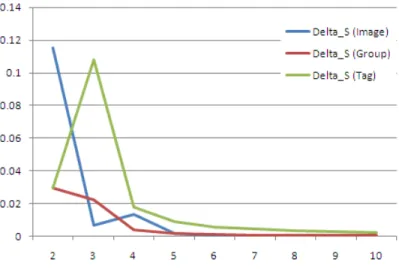
itera-tion. Y-axis denotes∆S(i.e.,Delta S). . . 34 3.15 Convergence of IWSL on Amazon data. X-axis denotes the number of

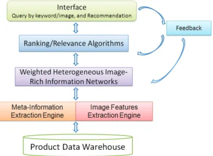
iteration. Y-axis denotes∆S(i.e.,Delta S). . . 34 3.16 Product search and recommendation system architecture. . . 35 3.17 Snapshot of the product search and recommendation system for e-commerce. 36 3.18 Recommendation comparison, ours v.s. Amazon’s ”Customers Who Bought

(11)

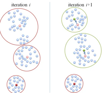
3.19 Recommendation comparison, ours v.s. Amazon’s ”Customers Who Bought This Item Also Viewed.” . . . 37 4.1 Active centers. In iteration i, there are three clusters, and the red points

indicate the cluster centers. At the next iterationi+1, two light red points are active centers because they move to different locations, while the solid red point is static. . . 42 4.2 Activity percentage curves for different number of clusters, based on dataset

VQDC. Horizontal axis denotes the number of iterations reached; vertical axis denotes the percentage of active centers at the specific iteration. Dif-ferent lines represent differentK, the number of clusters. . . 43 4.3 Activity percentage curves for different number of clusters, based on dataset

HDS-MTI. . . 43 4.4 How Boundary changes. (m=2) . . . 46 4.5 Illustrating how E-GAD works correctly for the case of Example 2. . . 50 4.6 Full Search area (shown in different colors). Horizontal axis denotes the

number of iterations reached; vertical axis denotes the percentage of Full Search points at the iteration. This result is based on dataset VQDC. . . 56 4.7 Full Search area (shown in different colors). Horizontal axis denotes the

number of iterations reached; vertical axis denotes the percentage of Full Search points at the iteration. This result is based on dataset HDS-MTI. . . . 57 4.8 Projection on the first three principle components for dataset VQDC. . . 64 4.9 Projection on the first three principle components for dataset KDDCUP04Bio.

There are some outliers, but most points lay on the right side. . . 64 4.10 Projection on the first three principle components for dataset MTI. . . 65 4.11 Projection on the first three principle components for dataset HDS-MTI. . . 65 4.12 Impact of parameter mon E-GAD for dataset VQDC. The horizontal axis

denotes the value ofm; the vertical axis denotes the Speedup over K-Means. 66 4.13 Impact of parametermon E-GAD for dataset HDS-MTI. The horizontal axis

denotes the value ofm; the vertical axis denotes the Speedup over K-Means. 66 4.14 Impact of parameter m on E-GAD for dataset KDDCUP04Bio. The

hori-zontal axis denotes the value of m; the vertical axis denotes the Speedup over K-Means. . . 66 4.15 Time performance of E-GAD, K-Means and GT on dataset VQDC.

Horizon-tal axis denotes the number of clusters; vertical axis denotes the Speedup over K-Means. . . 68 4.16 Time performance of E-GAD, K-Means and GT on dataset KDDCUP04Bio.

Horizontal axis denotes the number of clusters; vertical axis denotes the Speedup over K-Means. . . 68 4.17 Time performance of E-GAD, K-Means and GT on dataset HDS-MTI.

Hori-zontal axis denotes the number of clusters; vertical axis denotes the Speedup over K-Means. . . 69

(12)

4.18 Impact of parametermon approximate GAD algorithms. Horizontal axis denotes the value of m; vertical axis denotes the SDR or Speedup over E-GAD. The curves are based on dataset VQDC; other datasets have generally similar results. . . 70 4.19 Comparison of approximate GAD algorithms (NS-AGAD, S-AGAD,

I-AGAG and WB-AGAD) and CGAUCDB for dataset VQDC. Horizontal axis denotes the number of clusters; vertical axis denotes the Speedup over E-GAD. . . 71 4.20 Comparison of approximate GAD algorithms (NS-AGAD, S-AGAD,

I-AGAG and WB-AGAD) and CGAUCDB for dataset KDCUP04Bio. Hori-zontal axis denotes the number of clusters; vertical axis denotes the Speedup over E-GAD. . . 72 4.21 Comparison of approximate GAD algorithms (NS-AGAD, S-AGAD,

I-AGAG and WB-AGAD) and CGAUCDB for dataset HDS-MTI. Horizontal axis denotes the number of clusters; vertical axis denotes the Speedup over E-GAD. . . 72 4.22 Clustering quality comparison of approximate GAD algorithms (NS-AGAD,

S-AGAD, I-AGAG and WB-AGAD) and CGAUCDB for dataset VQDC. Horizontal axis denotes the number of clusters; vertical axis denotes the SDR over E-GAD. . . 73 4.23 Clustering quality comparison of approximate GAD algorithms (NS-AGAD,

S-AGAD, I-AGAG and WB-AGAD) and CGAUCDB for dataset HDS-MTI. Horizontal axis denotes the number of clusters; vertical axis denotes the SDR over E-GAD. . . 73 4.24 Speed degradation by RWFS, measured with Speedup. The horizontal axis

denotes the value ofR, and the vertical axis denotes the Speedup value. . . 74 4.25 Clustering quality improvement by RWFS, measured with SDR. The

hor-izontal axis denotes the value of R, and the vertical axis denotes the SDR value. . . 75 4.26 The like/favorite button for Facebook, YouTube, theAtlantic, Amazon and

Flickr, respectively. . . 80 4.27 A heterogeneous network model for social media with ‘like’ function, using

Facebook as an example. Abluebidirectional arrow is the friendship link. A red dashed arrow is a like action, while a green arrow denotes a post

action, annotated with the time stamp when it was posted. The dashed blue line shows that the two photos are visually similar. . . 81 4.28 LikeMiner System Architecture. . . 81 4.29 Heterogeneous Information Network for Social Media. A red face is a

spammer, a yellow smile face is a legitimate user, a yellow face turned to green color is an infected user. The blue directed line is the friend-ship/following link. A red arrow is a spam post, while a green arrow is a ham post. . . 83 4.30 SocialSpamGuard System Architecture. . . 84

(13)

5.1 An example of tweet about stock FB (Facebook Inc) posted by the user

Sarah Frier on June 6. . . 87

5.2 A 10-day change of FB stock price. . . 88

5.3 Graphical Model Representation of the Proposed Model. . . 90

5.4 Accuracy of the algorithms . . . 105

(14)

Chapter 1 Introduction

Web 1.0, designed by Tim Berners-Lee and released to the public in 1993, refers to the first stage of the World Wide Web (WWW) which provides a platform of information publishing that is read only. It mainly consists of static and non-interactive web pages made by companies, governments and a few individuals. There were 45 million global users on WWW in 1996.

Web 2.0 is represented by Social Media web applications that facilitate information publishing, sharing, interaction, user-centered design, and collaboration on the World Wide Web. A social media website allows users to create and upload user-generated con-tent and provides convenient ways to let them interact and collaborate with each other, in contrast to Web 1.0 websites where users are limited to the passive viewing of content that was created for them. Examples of social media websites include social networks (Facebook, LinkedIn, MySpace), blogs (Blogger) and microblogs (Twitter, Tumblr), wikis (Wikipedia), forums, reviews and news sharing (Digg), social tagging (or social book-marking) (Delicious), multimedia sharing (Flickr and YouTube), Social News, prediction markets, virtual worlds, online chatting (AIM, MSN, GTalk, QQ) and social online games. The Facebook website along had over 800 million users worldwide in 2011.

During the current age of social media, web usage can be characterized as the de-centralization of online information, which now largely consists of high volume and real-time content generated from the bottom-up, where common users are the contrib-utors and producers of information. The transition from Web 1.0 (represented by static webpages instead of dynamic user-generated content) to Web 2.0 (represented by Social

(15)

Media which consists of large scale of real-time and dynamic user-generated content), makes Internet information become in larger scale, richer, more interactive and complex. The phenomenal success of social media sites, such as Facebook, Twitter, LinkedIn, Flickr and YouTube, not only revolutionized the way people communicate and think, but also revolutionized the way how corporations do business.

The goal of this thesis is to mine the large scale user generated content in social media to explore the hidden relations and implications. Such analysis can be very useful for business, government, as well as individuals.

One basic problem for content relation analysis is content similarity. Content similarity computation is very important for many reasons, for example, grouping together simi-lar content can help better aggregate trends of topics for prediction, identifying simisimi-lar content objects can help recommendation in social media.

Documents and images are two major content information types in social media. How to compute document similarity and image similarity has been extensively studied in the information retrieval and computer vision areas. However, to compute similarity in such social media especially with image-rich network, is a very useful but also very challenging task, because there exists a lot of information such as text, image feature, user, group and most importantly thenetwork structure. Similarity of images is especially hard to estimate, because of the ”semantic gap” problem.

We propose an efficient approach called MoK-SimRank to significantly improve the speed of SimRank, which utilizes the network structure to estimate similarity, and in-troduce its extension HMok-SimRank to work on weighted heterogeneous information networks in social media. Then we propose algorithm IWSL to provide a novel way of integrating both link and content information. IWSL performs content and link reinforce-ment style learning with either global or local feature weight learning.

Another challenge for social media content mining is the large scale data. To deal with the problem, we propose a GAD (General Activity Detection) framework to fully explore

(16)

the power of activity detection for clustering. We design a set of algorithms within this framework for fast clustering in different scenarios. The most important contribution of our work is that GAD is the general solution to exploit activity detection for fast clustering and our algorithms within the framework can achieve very high speed.

Social media content not only relate to each other, but also to outside phenomena and show strong implication for prediction. Both governments and industries are interested in social trends. For example, politicians use polling to measure their popularity for elections and to monitor public sentiment to decide which position to take on social issues. Industry polls potential consumers to understand product acceptance. Although it is an expensive undertaking to perform polling, it is an investment that is critical for organizations both large and small to use for resource allocation and planning.

Social media provides a good platform to explore the global trends and sentiments that can be drawn by analyzing the general patterns of publishing/viewing/sharing con-tent objects in social media. In a sense, for example, each time a concon-tent object, such as a comment, image or video, is published or viewed, it constitutes an implicit vote for (or against) the subject of the content. This vote carries along with it a rich set of asso-ciated data including time and (often) location information. By aggregating such votes across millions of Internet users, we can develop prediction model to capture the wisdom that is embedded in social media sites for applications such as politics, economics, and marketing.

The rest of the thesis is organized as follows. In Chapter 2, we review related work. Chapter 3 describes our approach for similarity computation of both visual content and link information in a network setting. Chapter 4 presents our approach for conducting fast clustering on large scale data. Chapter 5 describes our unified model to integrate clustering, ranking and regression for prediction based on social media user content data. In Chapter 6, we conclude this thesis.

(17)

Chapter 2 Related Work

In this chapter, we review related work in existing literature.

2.1 Similarity Computation for Content Data

Document and images are two major content information types in social media. How to compute document similarity and image similarity has been extensively studied in the information retrieval and computer vision areas. Document similarity methods, such as vector space model and language model, has shown good success in identifying similar documents; however, image similarity is still a very hard task, because of the ”semantic gap” problem.

In text-based approach, image similarity is computed by the similarity of the text context, where estimating the similarity of the words in the context is useful for returning more relevant images. WordNet manually groups words into synonym sets, Google Distance [20] computes word similarity by co-occurrence in search results. Flickr Distance [114] considers visual relationship.

In image content-based approach, most methods (such as Google’s VisualRank [50]) and systems [106] [100] [37] [38] [87] [35] [15] [69] [109] [75] [54] compute image similarity based on image content features, such as RGB histogram and SIFT.

Hybrid approach combine text features and image content features together [24] [27] [89] [123]. Most commercial image search engines use textual similarity to return se-mantically relevant images and then use visual similarity to search for visually relevant

(18)

images.

Integration-based approaches [27] [89] [123] use linear or non-linear combination of the textual and visual features. However, existing works cannot handle the link structure. Among algorithms that compute object similarity considering link, SimRank [45] is one of the most popular. It computes node similarity based on the idea that ”two nodes are similar if they are linked by similar nodes in the network.” In spirit of PageRank [78], SimRank computes the similarity between each pair of nodes in an iterative fashion with a theoretical guarantee of the convergence. There are two problems of SimRank: (1) it is very expensive to calculate; and (2) the similarity is only based on the link information, when consider the images in the network, image similarity can actually also be judged by content features.

2.2 Fast Clustering on Large Set of Content Data

Performing efficient clustering on large content data is especially useful. There are ba-sically two strategies to develop fast clustering on large dataset. One is to develop fast core clustering algorithms, and the other is to develop pre-processing methods, such as sampling, subspace and compression, to reduce the dataset to a smaller size to achieve speedup. For example, CLARA [57] uses sampling strategies to reduce the size of data. BIRCH [128] compresses the original data using CF-tree and then employs the core clus-tering algorithm (e.g., K-Means) to perform the real clusclus-tering. In the thesis, we focus on developing fast core clustering algorithm.

K-Means [66] [70] is one of the most popular clustering algorithms, due to its high efficiency/effectiveness and wide implementation in many commercial/non-commercial softwares. The basic K-Means algorithm performs simple but effective clustering by iteratively partitioning a given dataset intoK clusters. For large-scale datasets, the ma-jor computation burden of K-Means clustering originates from the numerous distance

(19)

calculations between the patterns and the centers [58]. To deal with the problem, fast algorithms with different strategies have been proposed, such as PDS [8], TIE [19], Elkan [9], MPS [86], PAN [79], DHSS [99], FAUPI [62], kd-tree K-Means [81], AKM [83], HKM [76], GT [58] and CGAUCD [63]. Those algorithms come from several research communi-ties, such as data mining, machine learning, pattern recognition, multimedia processing and computer vision.

PDS (Partial Distortion Search) [8] cumulatively computes the distance between the pattern and a candidate center by summing up the differences in each dimension. If the dimensionality is high, PDS may still needs to compute many dimensions to stop accumulation. TIE (Triangular Inequality Elimination) [19] uses the triangle inequality condition for metric distance to prune candidate centers, thus reduces the number of distance calculations. TIE needs extra spaceO(K2_{) to save a distance matrix for the center}

vectors, and the entries are recalculated at the beginning of each partition. Elkan (by Charles Elkan) [9] is an exact fast algorithm for metric distance by using some metric distance properties. It needs to save the distances between every two centers and re-compute them at each iteration. The algorithm only works for metric distance, and is not scalable to largeK, the number of clusters, since it requires an additionalO(K2_{) complexity}

in both space and time. MPS (Mean-distance-ordered Partial Search) [86] is especially designed for Euclidean distance. MPS is faster thanK-Means if the improvement gained from pruning exceeds the overhead caused by sorting. PAN [79] rejects unlikely centers using mean values and variances of an input vector and its two sub-vectors. DHSS (Dynamic Hyperplanes Shrinking Search) [99] uses projection values of input vectors and centers on some dimensions to eliminate unlikely candidate centers. The DHSS algorithm with three projections has the less computing time than PAN. FAUPI [62] is another fast-searching algorithm using projection to reduce the dimension and inequality to reject unlikely codewords.

(20)

for metric distances. Kaukoranta et al. proposed algorithm GT [58] to utilize point activity for fast clustering and showed that it can further speedup PDS [8], TIE [19] and MPS [86]. Lai et al. proposed algorithm CGAUCD [63] as an extension of GT and demonstrated that combining CGAUCD with MFAUPI (which is an extension of FAUPI [62]) achieves the highest speed. Activity detection, which avoids the metric properties, works for both metric and non-metric distances.

2.3 Prediction Based on Social Media Content Data

James Surowiecki published the book ”The Wisdom of Crowds” [98], espousing the idea that under the right conditions, a crowd of non-experts can lead to decisions that are even smarter than the experts within the crowd. The conditions include independence of crowd members, decentralization, diversity and a means for aggregating the judgements of members. For a website with a large user base such as Flickr, all of these conditions are met.

Further, other work shows that the actions of individual Internet users, when properly pooled, can indicate macro trends. There are studies using Search Engine queries for influenza Internet surveillance [21], such as Google Trends [36], search advertisement click through [31], Yahoo search queries [84] and health website access logs [52].

Study on user web access logs from the Healthlink Web site [51] showed that there is a moderately strong correlation between the number of influenza-related article accesses and the CDC surveillance data.

Gunther [31] showed that there is a correlation between the number of clicks on keyword ”flu” or ”flu symptoms” triggered sponsored link in Google AdSense (appeared for Canadian searchers only) with epidemiological data from the flu season 2004/2005 in Canada.

(21)

Control (CDC) are used to find 45 specific search terms that are related to the percentage of influenze related physician visits. This model allows for monitoring influenza rates 1-2 weeksaheadof the CDC reports.

The problem of using general search engines is that the original query log is not publicly available and the query trends may become noisy under the impact of news events. For example, as soon as a new product is announced by a major technology company, blogs will begin to report and speculate about the product.

Joshua and Ewan [77] used prediction markets and Twitter to predict a swine flu pandemic. They ”explore the hypothesis that social media such as Twitter encodes the belief of a large number of people about some concrete statement about the world”. Such beliefs are aggregated using a Prediction Market specifically concerning the possibility of a Swine Flu Pandemic in 2009. They show that features extracted from Tweets can reduce the error associated with modeling these beliefs. The approach outperforms baseline methods based purely on time-series information from the Market.

Aron Culotta [22] studied how to detect influenza outbreaks by analyzing Twitter messages. Over 500 million Twitter messages were analyzed from an eight month period. The result showed that by tracking a small number of flu-related keywords, we are able to forecast future influenza rates with high accuracy, with a 95% correlation with national health statistics.

(22)

Chapter 3 Mutual Reinforcement based Content

Similarity Computation in Social Media

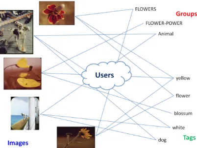
One basic problem for content relation analysis in social media is content similarity. In this chapter, we study the problem of how to conduct efficient and effective similarity computation considering the complex network property of social media.

Social multimedia (photo and video) sharing and hosting websites, such as Flickr, Facebook, YouTube, Picasa, ImageShack and Photobucket, are popular around the world, with over billions of photos uploaded by users. Popular Internet commerce websites such as Amazon are also furnished with tremendous amounts of product-related images. In addition, many images in such social networks are accompanied by information such as owner, consumer, producer, annotations and comments. They can be modeled as heterogeneous image-rich information networks. Figure 3.1 shows an example of the Flickr information network, where images are tagged by the users and image owners contribute images to topic groups. Figure 3.2 shows an Amazon information network of product images, categories and consumer tags.

Computing similarity in such large image-rich information networks is a very useful but also very challenging task, because there exists a lot of information such as text, image feature, user, group and most importantly the network structure. In text-based approach, estimating the similarity of the words in the context is useful for returning more relevant images. WordNet manually groups words into synonym sets, Google Distance [20] computes word similarity by co-occurrence in search results. Flickr Distance [114] considers visual relationship. In image content-based approach, most methods (such as Google’s VisualRank [50]) and systems [106] [100] [37] [38] [87] compute image similarity

(23)

Figure 3.1: Information network for Flickr, connected by images, user tags and groups.

Figure 3.2: Information network for Amazon, connected by products, user tags and categories.

based on image content features. Hybrid approach combine text features and image content features together [24] [27] [89] [123]. Most commercial image search engines use textual similarity to return semantically relevant images and then use visual similarity to search for visually relevant images. Integration-based approaches [27] [89] [123] use linear or non-linear combination of the textual and visual features. However, existing

(24)

works cannot handle the link structure. To solve the problem, we propose an image-rich information network model where the similarities between same type of nodes and different types of nodes can be better estimated based on the mutual impact under the network structure.

Among algorithms that compute object similarity in information networks, SimRank [45] is one of the most popular, but it is very expensive to calculate and the similarity is only based on the link information. When consider the images in the network, image similarity can actually also be judged by content features, such as color histogram, edge histogram and SIFT.

We propose an efficient approach called MoK-SimRank to significantly improve the speed of SimRank, and introduce its extension HMok-SimRank to work on weighted heterogeneous information networks. Then we propose algorithm IWSL to provide a novel way of integrating both link and content information. IWSL performs content and link reinforcement style learning with either global or local feature weight learning.

3.1 Preliminaries

We model a weighted heterogeneous image-rich information network as a graph G =

(V,E,W_{) with vertices}/_nodes_V_{, edges}_E_{and edge weights}W_. _V={_V_q}_{, where}_q =1, ...,_Q andQis the number of types of heterogeneous nodes,|_V_q|_{is the number of nodes of type}

i. Every image has aD-dimensional content featureF ∈_RD_{, which is either a single type}

of feature or a combination of multiple types of features. Add an edge li j ∈ E between

nodesi∈_V_and _j∈_V_{when they are linked together. Denote}$_{i j}_{as the weight of this link.} Without losing generality, we consider a heterogeneous network graph with three types of nodes (Q = 3): imagesVI, groups VG, and tags VT. Take Flickr network as an

example, there is an undirected link between an image nodee ∈_V_I_{and a tag node}_t∈ _V_T ifeis annotated witht, there is also an undirected link betweeneand a group nodeg∈ _V_G

(25)

ifebelongs to group g. There is no link between nodes of the same type. Table 3.1 lists the major notations.

Table 3.1: Major notations.

Notation Description

G graph model of image-rich information network

V the set of vertices/nodes in the graph

n n=|_V|_{, the total number of nodes}

VI the set of image nodes

VG the set of group nodes

VT the set of tag nodes

$i j the weight of a link in the graph.

I number of iterations for link-based algorithms K₍_c₎ _top_k_{similar candidates of object}_c

D number of dimensions for image feature

W a vector of weights for image feature

CW

i j weighted content similarity between imageiand j

G _{global regulated objective function} L _{local regulated objective function} F_{i j} _{confidence of the link between node}_i_and _j X_{i j} _theχ2 _{test statistic distance}

Ω() the sum of the weights

3.2 Fast Link-based Similarity

SimRank [45] is one of the most popular link-based algorithms for evaluating similarity between nodes in information networks. It computes node similarity based on the idea that ”two nodes are similar if they are linked by similar nodes in the network.” In spirit of PageRank [78], SimRank computes the similarity between each pair of nodes in an iterative fashion with a theoretical guarantee of the convergence. In a basic homogeneous network, SimRank computes the similarity score between two objectsoando0 is defined as, S(o,o0)= B |_N₍_o₎||_N₍_o0 )| X a∈_N(o) X b∈_N(o0 ) S(a,b) (3.1)

(26)

withB∈[0,_{1] as the damping factor,}_N₍_o_{) as the in-link nodes of}_o_,|_N₍_o₎|_{as the cardinality} of setN(o). There are two special cases: (1) if o= o0

, thenS(o,o0

) =1; and (2) if N(o) = ∅

orN(o0

)=∅, thenS(o,o0)=0.

For a network G of n nodes, the memory space needed by SimRank to store the similarity pairs is O(n2_{). Denote} _P _{as the time spending for calculating Equation 3.1,}

then the time complexity is O(n2_P_{) in a single iteration. Because SimRank is computed}

iteratively, the total time complexity is O(In2_P_{) for} _I_{iterations. The original SimRank is}

too computationally expensive to be used in large scale networks.

3.2.1 Mok-SimRank for Fast Computation

Some algorithms [45] [65] [33] [108] [124] have been proposed for more efficient SimRank computation. We use the pruning idea proposed by [45]. Initialize every object’s top

k(k _n_{) similar objects as candidates and focus computation on the chosen candidates.} This can reduce the space complexity to O(nk) and time complexity to O(InkP), and such method can be denoted ask-SimRank. We choose this strategy because it fits the property of large-scale image retrieval wherein most images are dissimilar to the query image and estimating their similarities many times is a waste. The time complexity of

Pink-SimRank isO(|_N₍_o₎||_N₍_o0

)|_log₍_k_{)), where}_log₍_k_{) is the complexity to decide whether}

Nj(o0) is a candidate of objectNi(o).

To make k-SimRank even more computationally efficient, we describe an approach called Mok-SimRank (minimum order k-SimRank). Denote K₍_c_{) as} _c_{’s top} _k _similar candidates. Between N(o) and N(o0

), denote Nbig as the neighborhood that has larger

cardinality andNsmallas the smaller one.

The basic idea of Mok-SimRank is that beginning with Nsmall, for every c ∈ Nsmall,

compute the scores considering two cases:

(27)

if false, get zero;

• _{Case 2 (}_k≥ |_N_big|_{): For}_d∈_N_big_{, check whether}_d∈ K₍_c_{). If true, return the score; else} if false, get zero.

The time complexity ofPis then reduced to be always the minimum combinationPmin,

Pmin =         

O(|_N_small|_klog₍|_N_big|₎₎ _: _{i f k}<|_N_big|

O(|_N_small||_N_big|_log₍_k₎₎ _: _{i f k}≥ |_N_big|

(3.2)

This is the optimal combination that achieves the minimum cost via automatically making the minimum computation order.

Table 3.2 summarizes the time and space complexity of the link-based similarity algo-rithms in a homogeneous network ofnnodes.

Table 3.2: Complexity of algorithms inHomogeneous Network. Algorithm Time Complexity Space Complexity

SimRank O(In2_P₎ _O₍_n2₎

K-SimRank O(InkP) O(nk)

Mok-SimRank O(InkPmin) O(nk)

3.2.2 HMok-SimRank for Weighted Heterogeneous Networks

Mok-SimRank can be extended to work for aweightedheterogeneous information network, which contains multiple types of nodes. To explain, we take the image-rich information network from Flickr as an example. Similar images are likely to link to similar groups and tags, so we define the link-based semantic similarity between imagese∈_V_I _and_e0 ∈_V_I_as follows, Sm+1(e,e 0 )=αISGm(e,e 0 )+βISTm(e,e 0 ) (3.3)

(28)

with SG_m(e,e0)= B G I Ω(NG₍_e₎₎∗Ω₍_NG₍_e0 )) X a∈_NG_(e) X b∈_NG_(e0 ) Ψab ee0S_m(a,b) (3.4) STm(e,e 0 )= B T I Ω(NT₍_e₎₎∗Ω₍_NT₍_e0 )) X a∈_NT_(e) X b∈_NT_(e0 ) Ψab ee0S_m(a,b) (3.5)

whereNG(e) is set of groups imageelinks to,NT(e) is set of tags imageelinks to. αI and

βI are the weights of link-based similarity for group and tag, respectively. We set both as

0.5 in experiment to treat them as equally important. BG

I andB

T

I are the damping factors.

Ω(NG₍_e_{)) is the sum of the weights for the links between image}_e_{and nodes in}_NG₍_e_),

Ω(NG(e))= X

a∈_NG_(e)

$ea (3.6)

Ψab

ee0is the importance/contribution ofS(a,b) forS(e,e 0

) considering the link weighting, and is defined as the multiplicative combination of the weights of the two linksleaandle0

b,

Ψab

ee0 =$_ea∗$_e0

b (3.7)

Weight $ can be set manually or automatically. The simplest case is that we set all weights to 1, then the network essentially becomes unweighted and all links are treated as equally important. However, in real applications, the links can be of non-equal importance. Take Amazon as an example, the tag frequency represents the number of users who think the tag is relevant to the product. So we can use the tag frequency (or log value) as weight$ea, for the link between product imageeand taga.

Similarly, we can define and compute the link-based group and tag similarity.

The group similarity is computed via the similarity of the images and tags they link to. For each pair of groupsg∈_V_G_and _g0 _∈

VG, Sm+1(g,g 0 )=αGSIm(g,g 0 )+βGSTm(g,g 0 ) (3.8)

(29)

with SI_m(g,g0)= B I G Ω(NI₍_g₎₎∗Ω₍_NI₍_g0 )) X a∈_NI_(g) X b∈_NI_(g0 ) Ψab gg0S_m(a,b) (3.9) STm(g,g 0 )= B T G Ω(NT₍_g₎₎∗Ω₍_NT₍_g0 )) X a∈_NT_(g) X b∈_NT_(g0 ) Ψab gg0S_m(a,b) (3.10)

where NI₍_g_{) is the set of images of group} _g_{, and} _NT₍_g_{) is set of tags of group} _g_{. The}

meaning and setting of parametersαG,βG,BI_GandBT_Gare similar to those in Equations 3.3,

3.4 and 3.5.

The tag similarity is calculated via the similarity of the images and groups they link to. For each pair of tagstandt0,

Sm+1(t,t0)=αTSIm(t,t 0 )+βTSGm(t,t 0 ) (3.11) with SIm(t,t 0 )= B I T Ω(NI₍_t₎₎∗Ω₍_NI₍_t0 )) X a∈_NI_(t) X b∈_NI_(t0 ) Ψab tt0S_m(a,b) (3.12) SG_m(t,t0)= B G T Ω(NG₍_t₎₎∗Ω₍_NG₍_t0 )) X a∈_NG_(t) X b∈_NG_(t0 ) Ψab tt0S_m(a,b) (3.13)

where NI₍_t_{) is the set of images tagged by}_t_{, and} _NG₍_t_{) is set of groups tagged by} _t_{. The}

meaning and setting of parametersαT,βT,BI_T andBG_T are similar to those in Equations 3.3,

3.4 and 3.5.

The similarity score for any pair of nodes within the same type is initialized as 0 for different nodes and 1 for the same node. We do not consider similarity between nodes from different types.

The similarity scores in Equations 3.4, 3.5, 3.9, 3.10, 3.12 and 3.13 can be efficiently computed by the idea introduced in Mok-SimRank. So we can still achieve high efficiency via Mok-SimRank for heterogeneous networks. Notethat the computation of the similarity scores in Equations 3.3, 3.8 and 3.11 are mutually dependent.

(30)

Generally, basic SimRank, K-SimRank and Mok-SimRank can be extended to compute link-based similarity in (weighted) heterogeneous networks, and we call themHSimRank andHK-SimRankandHMok-SimRankto distinguish with the situation in homogeneous networks.

Table 3.3 summarizes the time and space complexity of the link-based similarity algo-rithms in a (weighted) heterogeneous network ofp types of nodes, with mi(i ∈ {1, ...,p})

nodes for typei. Note that the total number of nodes in the network isn=Pp

i=1mi.

Table 3.3: Complexity of algorithms in (weighted)Heterogeneous Network. Algorithm Time Complexity Space Complexity

HSimRank O(IPp i=1m2iP) O( Pp i=1m2i) HK-SimRank O(IPp i=1mikP) O(P_i=1p mik)=O(nk) HMok-SimRank O(IPp i=1mikPmin) O( Pp i=1mik)=O(nk)

3.3 Weighted Content-based Similarity

Image similarity can be estimated from image content features [24] [26] [122], such as color histogram, edge histogram [68], Color Correlogram [42], CEDD [18], GIST, texture features [2] [73] , Gabor features [80] [92], shape [43] [60]and SIFT [67].

We represent an image as a point in a D-dimension feature space with either a single type of feature or a combination of multiple types of features. Tang at el. proposed strategies to integrate both local and global features [101]. If the integrated feature space has fixed number of dimensions, our approach is also applicable.

Normalize featureF∈ _RD_{, where}_D_{is the number of dimensions in the feature space,} to be of unit length: for any fd_{, the value of feature}_F_{on dimension}_d₍_d₌_{1, ...,}_D_{), divide}

it by the sum of values on all dimensions.

fd= f_origd .

D

X

d=1

(31)

Theχ2_{test statistic distance between two feature vectors}_F

i andFjis defined as:

X_{i j} ≡ X₍_F_i,_F_j₎ ≡ D X d=1 cd_{i j} (3.15) = 1 2 D X d=1 (f_id− _fd j) 2 fd i + fjd (3.16)

When feature vectors are normalized to unit length, theχ2_{test statistic distance varies}

from 0 to 1, with 0 indicating the most similar and 1 indicating the most different.

Existing studies on metric learning [120] [116] [113] have empirically and theoretically shown that instead of treating each dimension of the feature vector equally, a learned weighted metric can significantly improve the performance for tasks such as image re-trieval [120], classification [6] and clustering [119]. This is because the feature dimensions are usually not equally important for measuring the similarity between images. We can obtain better result by putting more weights on a subset of features, which are more relevant to the semantic meaning of the images.

Based on the χ2 _{test statistic distance and a}_D_{-dimensional feature weighting vector}

W = (w1_,_w2_{, ...,}_wD_{), we define the weighted content similarity}_CW

i j between images iand

jas follows: CW_{i j} ≡ ₁−1 2 D X d=1 (wd_fd i −w d_fd j) 2 wd_fd i +wdf d j (3.17) = 1− D X d=1 wdcd_{i j} (3.18)

which is used to evaluate the image similarity. There are two reasons why we chooseχ2_:

Firstly, it has shown performance as good as, and sometimes better, with cosine,L1 andL2 measures for image similarity in our experiments by human judgment. It has been used in image retrieval [10] [107] and obtains best accuracy as a kernel for SVM-based image classification [104] [46] [127]. Secondly, its sum of square formula makes it convenient to

(32)

perform Gradient Decent-based optimization used in our algorithm as described in the next section.

3.4 Reinforced Integration of Link and Content

Similarities

Using content similarity only may lead to unsatisfying results. Figure 3.3 shows one pair of Flickr images that have similar content similarity estimated from the low-level feature, but with different semantic meaning.

Figure 3.3: Images with high visual similarity, but low semantic similarity.

Direct use of link information solely based on human annotations may also lead to unsatisfying results if the annotation is wrong, too general, or incomplete. In addition, if the image does not link to any object in the information network, then only based on link information cannot work.

Figure 3.4 shows several examples that are all linked to tag ”flower” but they are not visually similar.

Traditional thinking is to combine content and link information to achieve more robust performance. In this section, we describe a novel way to integrate these two types of information.

(33)

Figure 3.4: Images annotated by the tag ”flower”, but with low visual similarity.

3.4.1 Learning the Feature Weights

To build a bridge between the content and semantics, we learn a weighting vectorW ∈_RD for the feature space to force the weighted content-based similarityCW_{i j} to be somehow con-sistent with the semantic link-based similaritySi j. We consider two types of approaches:

global feature learning and local feature learning.

Global Feature Learning (GFL)We minimize the following regulated objective func-tion to findW, G₍_W,_p,_h₎=β||_W||2+ |_V_I| X i=1 X j∈K_(i) Y_{i j} _(3.19)

where|_V_I|_{is the number of images and}K₍_i_{) is the set of top}_k_{neighboring candidate images} of imagei, by combining both topk/2 most visually similar and topk/2 most semantically

similar images. The first componentβ||_W||2_{is a}_L

2regulation. The second componentYi j

serves as the bridge between content-based similarity and link-based similarity,

Y_{i j} = ₍_CW i j −(pSi j+h))2Fi j = (1− D X d=1 wdcd_{i j}−₍_pS_{i j}+_h₎₎2F_{i j} _(3.20) whereCW

i j (defined in Equation 3.17) andSi j(defined in Equation 3.3) may have different

(34)

If the tags (or groups) of an image are incomplete (0 or very few) and thus cannot fully describe its semantic meaning, the link-based similarity becomes less reliable. In order to consider this factor, we introduceF_{i j}_{as the confidence (or importance) of}_S_{i j}_{, and define} it as a function of the number of linked annotations (including both tags and groups) to the imagesiand j,

F_{i j} =₁−_e−τΓi j _(3.21)

where Γi j is defined as the minimum number of links (including tags and groups) for

imageiand j, i.e.,

Γi j =min

n

|_NT₍_i₎+_NG₍_i₎|,|_NT₍_j₎+_NG₍_j₎|o. _(3.22) Parameter τ rescales the value of Γi j to adjust the importance of count. It can be either

manually set or automatically estimated by the average ofΓi jvalues.

The value of F_{i j} _{varies from 0 to 1, with 1 indicating the highest confidence and 0} indicating the lowest confidence. IfΓi j = 0 (i.e., at least one of images does not have any

tag and group), thenF_{i j} =_{0, which means the link-based similarity is not reliable because} the semantic information given by human annotation is missing.

Note that we can also use graph ranking algorithms, such as PageRank [78] and HITS [17], to estimate the importance of a node, instead of simple counting. In addition, we may also consider thet f ∗_{id f} _{score of tags, similar to document retrieval, to give higher} weights to topic terms and lower weights to general terms.

The overall importanceF_S_{is defined as}

F_S= |_V_I| X i=1 X j∈K_(i) F_{i j} _(3.23)

By consideringF_S_{, we obtain the following new global objective function,}

G₍_W,_p,_h₎=β||_W||2+ 1 F_S |_V_I| X i=1 X j∈K_(i) Y_{i j} _(3.24)

(35)

whereβis the weight of the regulator. To find (W∗_,

p∗_, h∗

) that minimizes the above objective function, we first compute the first-order partial derivatives,

∂G ∂wd =2βw d₊ 1 F_S |_V_I| X i=1 X j∈K_(i) 2F_{i j}₍₁− D X d=1 wdcd_{i j}−₍_pS_{i j}+_h₎₎₍−_cd i j) (3.25) ∂G ∂p = 1 F_S |_V_I| X i=1 X j∈K_(i) 2F_{i j}₍₁− D X d=1 wdcd_{i j}−₍_pS_{i j}+_h₎₎₍−_S_{i j}₎ _(3.26) ∂G ∂h = 1 F_S |_V_I| X i=1 X j∈K_(i) 2F_{i j}₍₁− D X d=1 wdcd_{i j}−₍_pS_{i j}+_h₎₎₍−₁₎ _(3.27) The variables are estimated by Gradient Decent (or Stochastic Gradient Decent, which could be faster) iteratively,

wd_m+1 =wdm−γwd ∂ G ∂wd _wd_=wd m f or all d ∈ {1, ...,_D} _(3.28) pm+1=pm−γp∂ G ∂p _p₌_p m (3.29) hm+1=hm−γh ∂G ∂h _h=h m (3.30) wheremdenoted them-th iteration.

After global feature learning, based on the new feature weighting, update the image similarity as a combination of content-based and link-based similarity,

S(i,j)=(1−µ)_CW∗ i j +µ(p ∗ Si j+h ∗ ) (3.31)

where parameterµ∈[0,_{1] controls the weight of link-based similarity in the combination.} We could manually set a value based on user preference or automatically use the value of F_{i j} _{which estimates the confidence score of the link-based similarity, as defined in}

(36)

Equation 3.21.

Local Feature Learning (LFL) The problem of global feature learning is that using a global feature weighting for all images may be too general. Different images may belong to different semantic topics and thus need different weightings to capture their specific important features. Therefor, we can perform local feature learning (LFL) to find a specific feature weightW∗

i for imagei. More specifically, for each imagei, we learn a local weight

Wi, which minimizes the following objective functionLi,

L_i₍_W,_p,_h₎ = β||_W||2+ 1 Fi S X j∈K(i) Y_{i j} _(3.32) = β||_W||2+ X j∈K_(i) (CW i j −(piSi j+hi)) 2_F i j Fi S where Fi

S is the normalization factor to sum up the importance of all pairs for image i,

and is defined as Fi S = X j∈K_(i) F_{i j} _(3.33)

Similar to GFL, in order to find parameters (W∗_, p∗_,

h∗

) for imagei that minimizes its objective function, we first compute the first-order partial derivatives,

∂L_i ∂wd =2βw d₊ 1 Fi S X j∈K_(i) 2F_{i j}₍_CW i j −(pSi j+h))(−c d i j) (3.34) ∂L_i ∂p = 1 Fi S X j∈K_(i) 2F_{i j}₍_CW i j −(pSi j+h))(−Si j) (3.35) ∂L_i ∂h = 1 Fi S X j∈K_(i) 2F_{i j}₍_CW i j −(pSi j+h))(−1) (3.36)

Use Gradient Decent to compute parameters iteratively using the following formula,

wd_m+1 =(1−₂γ_wdβ)wd_m+γ_wd 1 Fi S X j∈K_(i) 2F_{i j}₍_CWm i j −(pmSi j+hm))c d i j (3.37)

(37)

pm+1 =pm+γp 1 Fi S X j∈K_(i) 2F_{i j}₍_CWm i j −(pmSi j+hm))(Si j) (3.38) hm+1 =hm+γh 1 Fi S X j∈K_(i) 2F_{i j}₍_CWm i j −(pmSi j+hm))) (3.39)

Because the weights have similar properties, we set allγ_wd as the same: γ_w. Then the number ofγ_{parameters is reduced from}_D+_{2 to 3. We initialize the variables as follows,}

wd

0 =1 (for alld=1, ...,D),p0 =1 andh0 =0.

After local metric learning, based on the learned local weights, the similarity between two imagesiand jcan be computed in two ways: symmetric and asymmetric.

The asymmetric similaritySA₍_i_,_j_{) is defined as}

SA(i,j)=(1−µ)_CW ∗ i i j +µ(p ∗ iSi j+h ∗ i) (3.40)

where (Wi,pi,hi) are the learned parameters for imagei.

The symmetric similaritySS₍_i_, _j_{) is defined as}

SS(i,j)= S

A₍_i_,_j₎₊_SA₍_j_,_i₎

2 (3.41)

3.4.2 Integration Algorithm

We present novel algorithm to integrate link-based and content-based similarities. A basic approach would be in two-stage: firstly perform HMok-SimRank to compute the link-based similarities and secondly perform feature learning (either GFL or LFL) consid-ering the link-based similarity to update the feature weights, and then update the node similarities based on the new content similarity. Algorithm 1 describes the procedure of the Two-Stage approach.

In the Two-Stage approach, image content similarity is not used to help upgrade tag and group similarities. To solve this problem, we need an algorithm that can provide

(38)

Algorithm 1Two-Stage Approach

Require: G, the image-rich information network. 1. Find topKsimilar candidates of each object; 2. Initialization;

3. Iterate{

4. Compute link similarity for all image pairs; 5. Compute link similarity for all group pairs; 6. Compute link similarity for all tag pairs; 7. }until converge or stop criteria satisfied; 8. Perform feature learning to updateW =W∗

m+1;

9. Update image similarities by Equation 3.31 (global), or 3.40, 3.41 (local); Ensure: S, pair-wise node similarity scores.

deeper integration between content and link information. The idea is that after feature learning, we update the image similarity by combining the link similarity with weighted content similarity. (Before going to the next step, one option is to use the new similarity to update the set of similar candidates by introducing more candidates that may have been missed in the initialization step.) Based on the new image similarity, we can update the group and tag similarity. With new tag and group similarity, we can update new link-based image similarity and learn a new weight. The image/tag/group similarities will be mutually updated iteratively until the process converges or any stop criteria is satisfied. We call this approach Integrated Weighted Similarity Learning (IWSL). The termweighted

has two meanings: (1) we learn weighted content feature, and (2) the algorithm works in a general weighted heterogeneous network. Algorithm 2 describes the procedure of IWSL.

Table 3.4 summarizes the time and space complexity of Two-Stage and IWSL in a (weighted) heterogeneous network ofp types of nodes, where there are mi(i ∈ {1, ...,p})

nodes for type i and the total number of nodes is n = Pp

i=1mi. Let J be the number of

iterations for Gradient Decent iterative updating, thenQ = O(J|_V_I|_k_{) is time complexity} for feature learning (both GFL and LFL are the same). Denotevas the number of variables to be estimated. For GFL,v=D+2, and for LFL,v=|_V_I|₍_D+_2).

(39)

Algorithm 2Integrated Weighted Similarity Learning (IWSL) Require: G, the image-rich information network.

1. Constructkd-tree [12] (or LSH [23] andcv-tree [13] index) over the image features; 2. Find topk(or-range) similar candidates of each object;

3. Initialize similarity scores; 4. Iterate{

5. Calculate the link similarity for image pairs via HMok-SimRank; 6. Perform feature learning to updateW = W∗

m+1, using either global or local feature

learning;

7. (Optional) Search for new topksimilar image candidates based on the new similarity weighting;

8. Update the new image similaritiesSm+1(i,i0) by Equation 3.31 (global), or 3.40, 3.41

(local);

9. Compute link-based similarity for all group and tag pairs via HMok-SimRank; 10. }_{until converge or stop criteria satisfied.}

Ensure: S, pair-wise node similarity scores.

Table 3.4: Complexity of Two-Stage and IWSL inHeterogeneous Network. Algorithm Time Complexity Space Complexity

Two-Stage O(J|_V_I|_k+_I₍Pp

i=1mikPmin)) O(nk+v)

IWSL O(IJ|_V_I|_k+_IPp

i=1mikPmin)) O(nk+v)

3.5 Experiments

Experiments were conducted on a PC with Intel Pentium(R) D 3.4GHz CPU and 4GB RAM, running Windows XP.

3.5.1 Datasets

We conduct experiments on two datasets: Flickr and Amazon. The Flickr dataset is created by downloading the images and related meta-data information, such as groups and tags using Flickr API. The Amazon dataset is created by downloading product images and related meta-data information, such as category, tags and title, via the API of Amazon. The Amazon API only returns the top 5 tags for each product, so we use the words in the title as additional tags. Product category is treated as group. Table 4.3 shows the statistics for the two datasets.

(40)

Table 3.5: Statistics for the datasets Datasets Images Groups Tags Links

Flickr 14,559 24 23,420 298,376 Amazon 118,426 41 56,914 1,307,092

For image feature extraction, we extracted CEDD [18], which is a compact descriptor that considers both color and edge features. In literature, it has shown good performance compared with many traditional features. Note that our model is general to other features or combination of them.

Tag Preprocessing. We change all tags to lower case. Tags with only number characters

are removed. Stop-words, such asthe,youandme, are also removed. The remaining tags are stemmed using the Porter stemming algorithm [85]. We remove very infrequent tags and only retain those that appear in more thank(e.g.,k=2) images.

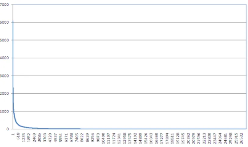
Figure 3.5 shows the tag frequency (the number of images annotated with the tag) of dataset Flickr. We can observe that many tags have low frequency, and a very few tags have high frequency. The Amazon dataset has similar curve shape, as shown in Figure 3.6.

Figure 3.5: Tag frequency for the Flickr dataset. Y-axis denotes the frequency, X-axis denotes the ordered (by frequency) tag id.

(41)

Figure 3.6: Tag frequency for the Amazon dataset. Y-axis denotes the frequency, X-axis denotes the ordered (by frequency) tag id.

Table 3.6: Top 10 most frequent tags. (a) Flickr Tag Frequency flower 1970 nikon 1545 night 1491 white 1468 black 1288 canon 1252 geotag 1250 light 1231 sky 1127 nature 1122 (b) Amazon Tag Frequency black 6088 pack 4621 case 4235 watch 3987 women 3706 men 3611 classic 3348 music 3321 set 3231 game 3228

3.5.2 Performance Results

Figure 3.7 shows the speed-up (Tbaseline/Ti) of HK-SimRank and HMoK-SimRank over

baseline HSimRank. With the increase of the number of images, they become increasingly faster than HSimRank. Note that we only show result for as most 3000 images due to the expensive time complexity of the baseline HSimRank, which takes too long for larger data. Figure 3.8 shows the speed-up of HMoK-SimRank over HK-SimRank. We can see that HMoK-SimRank is much faster than HK-SimRank. Because IWSL is based on HMoK-SimRank, it has similar time efficiency except for the time spent on feature weight

(42)

learning.

For exact executing time, we take the Amazon dataset as an example: when the number of images is 3000, HSimRank takes 598 seconds, HK-SimRank takes 24 seconds and HMoK-SimRank takes 9 seconds; when the number of image increase to 20000,HK -SimRank takes 928 seconds, while HMoK--SimRank only takes 132 seconds.

Figure 3.7: Speed-up of HK-SimRank and HMok-SimRank over HSimRank. X-axis de-notes the number of images, Y-axis dede-notes the speed-up (in times ratio).

Figure 3.8: Speed-up of HMok-SimRank over HK-SimRank. X-axis denotes the number of images, Y-axis denotes the speed-up (in times ratio).

Because of the large number of images, it is difficult to check one by one to obtain a complete set of relevant images for each query image. In order to generate an approximate ground truth for performance evaluation, we assume that if two images are relevant, their visual similarity should be above a threshold εv and the number of shared tags should

(43)

also be above a thresholdεt.

We ignore images which contain less than 5 tags. Such images make up 6.5% and 15.3% of the Flickr and Amazon dataset, respectively. Since all considered images have more than 5 tags, which are human annotations, if two images don’t have any common tag, it is likely that the users who made those tags do not think they are relevant. On the Internet, there are many images do not have tags, to simulate the real world case, we randomly select 50% images to remove all their tags. Our algorithm can still find some of them as relevant because we are able to learn a feature weight based on those images which have tags or other link-based information.

We compare VLWC (weighted combination of visual and link similarity without fea-ture weight learning), IWSL L (IWSL with local feafea-ture weight learning) and IWSL G (IWSL with global feature weight learning) to several baselines: Visual (only use the vi-sual similarity), Text (only use the textual similarity, following a popular text retrieval ap-proach: cosine measure based on thet f ∗_{id f} _{weighted tag vector), VTWC [27] (weighted} combination of visual and textual similarity, we choose equal weight), Link (HMok-SimRank which only use the link similarity), MinFusion and MaxFusion [27].

Evaluation method: we use mean average precision (MAP) to measure the retrieval

performance of the algorithms. For every image in the dataset, we obtain a ranking list of relevant images computed by each algorithm and compute the average precision based on the approximate ground truth before removing tags. The final MAP score for each algorithm is calculated as the mean average precision of each image. Note that there is no training data. So all the algorithms are un-supervised.

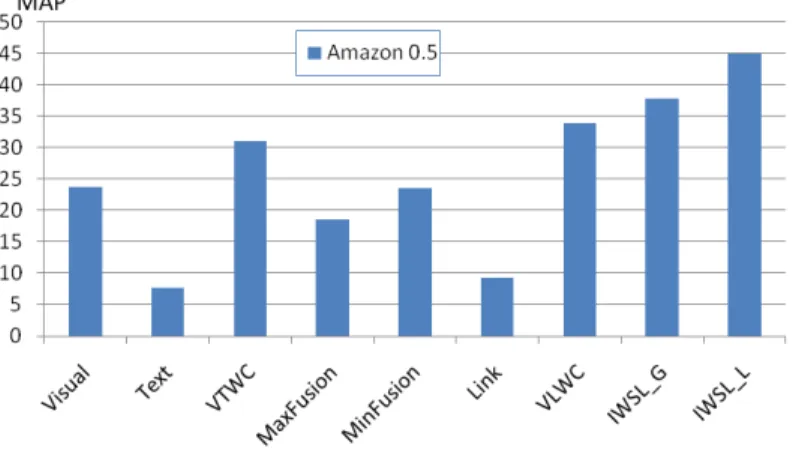
Figures 3.9 and 3.10 show the result on Flickr and Amazon data, respectively. We can see that link-based similarity performs better than text-based similarity; VLWC achieves better performance than traditional algorithms by linearly combining visual and link information together. Algorithm IWSL further improves the performance by introducing a new way of integrating content and link information via mutual reinforcement with

(44)

feature learning. IWSL L achieves better results than IWSL G, because IWSL L performs local feature learning, which can find a specific and better feature weighting for each image than global feature learning, which finds a general feature weighting for all images.

Figure 3.9: MAP of the algorithms on Flickr data. X-axis denotes the algorithms. Y-axis denotes the MAP (%).

Figure 3.10: MAP of the algorithms on Amazon data. X-axis denotes the algorithms. Y-axis denotes the MAP (%).

Case Study:

As an example from the Flickr dataset, Figure 3.11 shows the top 10 most similar images for a query image about ”moon,” using link-based (SimRank) (1st row), content-based similarity (2nd row), and IWSL (3rd row), respectively. The top left image is the

(45)

query image. Clearly, IWSL obtains the most relevant matches for both semantic and visual appearances.

Figure 3.11: Top 10 retrieval results by (1) Link (SimRank), (2) Content similarity, and (3) IWSL. The top left image is the query image from the Flickr dataset. It is tagged with ”moon, lune, sky” and belongs to group ”After Dark - Night Photography.”

In another example from the Amazon dataset, Figure 3.12 shows the top 10 most similar images for a query image about ”iPhone,” using link-based similarity (SimRank) (1st row), content-based similarity (2nd row), and IWSL (3rd row). Again, IWSL obtains the best results in terms of the relevance for both semantic and visual appearances.

Figure 3.12: Top 10 retrieval results by (1) Link (SimRank), (2) Content similarity, and (3) IWSL. The top left image is the query image from Amazon. It is tagged with ”iPhone, invisible shield, accessories” and belongs to category ”WirelessAccessories.”