Bayesian inference for continuous time Markov chains

(1)

Alharbi, Randa (2019) Bayesian inference for continuous time Markov

chains. PhD thesis.

https://theses.gla.ac.uk/40972/

Copyright and moral rights for this work are retained by the author

A copy can be downloaded for personal non-commercial research or study,

without prior permission or charge

This work cannot be reproduced or quoted extensively from without first

obtaining permission in writing from the author

The content must not be changed in any way or sold commercially in any

format or medium without the formal permission of the author

When referring to this work, full bibliographic details including the author,

title, awarding institution and date of the thesis must be given

Enlighten: Theses https://theses.gla.ac.uk/ [email protected]

(2)

Time Markov Chains

A thesis submitted to the University of Glasgow in fulfilment of the requirements for the award of the degree of Doctor of

Philosophy in the College of Science and Engineering

Randa Alharbi

School of Mathematics and Statistics

University of Glasgow

(3)

Abstract

Continuous time Markov chains (CTMCs) are a flexible class of stochastic models that have been employed in a wide range of applications from timing of computer protocols, through analysis of reliability in engineering, to models of biochemical networks in molecular biology. These models are defined as a state system with con-tinuous time transitions between the states. Extensive work has been historically performed to enable convenient and flexible definition, simulation, and analysis of continuous time Markov chains. This thesis considers the problem of Bayesian pa-rameter inference on these models and investigates computational methodologies to enable such inference. Bayesian inference over continuous time Markov chains is particularly challenging as the likelihood cannot be evaluated in a closed form. To overcome the statistical problems associated with evaluation of the likelihood, ad-vanced algorithms based on Monte Carlo have been used to enable Bayesian inference without explicit evaluation of the likelihoods. An additional class of approximation methods has been suggested to handle such inference problems, known as approxi-mate Bayesian computation. Novel Markov chain Monte Carlo (MCMC) approaches were recently proposed to allow exact inference.

The contribution of this thesis is in discussion of the techniques and challenges in implementing these inference methods and performing an extensive comparison of these approaches on two case studies in systems biology. We investigate how the algorithms can be designed and tuned to work on CTMC models, and to achieve an accurate estimate of the posteriors with reasonable computational cost. Through this comparison, we investigate how to avoid some practical issues with accuracy and computational cost, for example by selecting an optimal proposal distribution and introducing a resampling step within the sequential Monte-Carlo method. Within the implementation of the ABC methods we investigate using an adaptive tolerance schedule to maximise the efficiency of the algorithm and in order to reduce the computational cost.

(4)

I declare that all the work presented in this thesis has been done by myself under the supervision of Dr. Vladislav Vyshemirsky and Prof. Dirk Husmeier, except where otherwise stated. This thesis represents work completed, between 2014 and 2018 in Statistics in the School of Mathematics and Statistics at the University of Glasgow.

©Randa Alharbi, 2018.

(5)

Acknowledgements

A huge thank my supervisor Dr.Vladislav Vyshemirsky for his scientific guidance, support and encouragement over the duration of my PhD. Without him, this work would have never been accomplished. I truly could not have hoped for better super-visor. I am deeply grateful to you, Dr.Vlad.

Many thanks to Prof.Dirk Husmeier, for for discussions, scientific guidance and general support.

I want to thank my examiners, Prof.Guido Sanguinetti and Dr.Vincent Macaulay for providing valuable suggestions.

I also would like to thank the academic staff of the school for providing a good and friendly environment for the Ph.D. students. Special thanks to Prof. Adrian Bowman for his help, support and advice.

I owe thanks to Heather Lambie (Graduate School Manager) and her team for their administrative guidance during my PhD.

A big thanks to my colleague Suzy Whoriskey and Eilidh Jack, they have been amazing company. I also would like to thank my friends Amani, Salihah, Shuhrah for their love and kindness.

A lot of thanks to the Ministry of Higher Education and my employer Tabuk Uni-versity for funding my work. I would like also to thank the Saudi Arabian Cultural Bureau for their help and support throughout my study.

Many thanks for my parents and family for their love, prayers, support and encour-agement. And most of the thanks to my kids and my husband for love, support and being patient.

(6)

List of Figures ix

List of Tables xx

List of Algorithms 1

1 Introduction 2

1.1 Introduction and Thesis Statement . . . 2

1.2 Thesis Contribution . . . 4

1.3 Outline of the Thesis . . . 5

2 Markov Chains 6 2.1 Stochastic Process . . . 7

2.2 Markov Chains in a Discrete State Space . . . 7

2.2.1 Transition Matrix . . . 8

2.2.2 Chapman-Kolmogorov Equation . . . 8

2.3 State Probabilities . . . 10

2.3.1 Important Properties and Classification of States in a Markov Chain . . . 12

2.3.2 Recurrence and Transience . . . 13

2.3.3 Time Reversible Markov Chain . . . 15

2.4 Continuous Time Markov Chains . . . 16

2.5 An Overview of Modelling Biological Systems . . . 18 iv

(7)

Contents v

2.5.1 Stochastic Biochemical Kinetic . . . 19

2.5.2 The Markov Description of Biochemical Reaction Network . . 20

2.5.3 The Chemical Master Equation . . . 22

2.5.4 Stochastic Simulation . . . 24

2.6 Related Works . . . 24

2.6.1 Exact Methods . . . 24

2.6.2 Approximate Methods . . . 29

2.7 Summary . . . 32

3 Bayesian Inference Methods 33 3.1 Monte Carlo Methods . . . 35

3.1.1 Rejection Sampling . . . 36

3.1.2 Importance Sampling . . . 38

3.2 Sequential Monte Carlo Methods . . . 39

3.2.1 Sequential Importance Sampling . . . 40

3.2.2 Particle Degeneracy . . . 41

3.2.3 Sequential Importance Resampling . . . 42

3.2.4 Bayesian Inference with a State Space Model . . . 45

3.2.5 Bootstrap Particle Filter . . . 49

3.3 Markov Chain Monte Carlo . . . 49

3.4 Metropolis-Hastings . . . 51

3.5 Optimal Choice of Proposal for the MH . . . 57

3.5.1 Methods for Monitoring Convergence . . . 59

3.6 Pseudo-Marginal MCMC . . . 65

3.7 Particle Markov Chain Monte Carlo . . . 67

3.8 Exact Inference . . . 69

3.8.1 Sampling a Trajectory . . . 69

(8)

3.8.3 Russian Roulette . . . 71

3.8.4 Expanding the Likelihood . . . 72

3.8.5 Modified Gibbs Sampler . . . 72

3.9 Related Work . . . 73

3.10 Summary . . . 75

4 Approximate Bayesian Computation 77 4.1 Introduction . . . 77

4.2 Review of Likelihood-Free Methods . . . 77

4.3 ABC Rejection . . . 82

4.4 Sequential Approximate Bayesian Computation Approach . . . 85

4.5 ABC SMC Algorithm Tuning . . . 87

4.5.1 Tolerance Level . . . 87

4.5.2 Perturbation Kernel . . . 88

4.5.3 Number of Particles . . . 89

4.5.4 Target Tolerance and the Number of Stages . . . 89

4.5.5 Effective Sample Size . . . 90

4.6 Summary . . . 91

5 Application to the Lotka-Volterra Model 93 5.1 The Lotka-Volterra Model (LV) . . . 94

5.2 Simulation of the Lotka-Volterra Model . . . 96

5.2.1 Changing the Reaction Rate Parameters . . . 98

5.2.2 The Effect of Varying the Prey Production Rate c1 . . . 98

5.2.3 The Effect of Varying the Predator Death Rate c2 . . . 100

5.2.4 The Effect of Varying the Predator Death Rate c3 . . . 100

5.3 Parameter Inference . . . 101

(9)

Contents vii

5.5 Further Investigation . . . 109

5.6 Application of the PMMH on the LV Model . . . 113

5.7 Comparison . . . 118

5.7.1 Improving the Performance of the PMMH Algorithm . . . 125

5.8 Application of Approximate Bayesian Computation on a Larger Data Set . . . 129

5.8.1 Further Analysis . . . 132

5.9 Summary . . . 134

6 Application to Repressilator System 138 6.1 Repressilator System . . . 139

6.2 Model Reactions . . . 140

6.3 Simulating CTMC Trajectories . . . 142

6.4 Inference Based on Synthetic Data . . . 143

6.4.1 Exact Inference . . . 144

6.4.2 Application of the ABC SMC . . . 150

6.4.3 Application of the PMMH to the Repressilator Model . . . . 154

6.5 Parameter Inference for Repressilator Model Using Real Data . . . . 164

6.6 Summary . . . 168

7 Summary and Conclusion 172 7.1 Limitations and Further Improvement . . . 174

7.2 Software Implementation . . . 175

Appendices 176 A Additional Result from the Gibbs Sampler 177 A.1 Forward-Backward Algorithm . . . 177

(10)

B Implementation Details 183

C Additional Results for LV Model Parameter Inference 185

D Several Simulation from the LV Model 189

E Additional Result for the Repressilator Model 191

(11)

List of Figures

3.1 The plot shows the histogram of samples from the beta distribution produced with the MH algorithm and the red line shows the proba-bility density of our target distribution. The histogram matches the target distribution reasonably well. . . 55 3.2 The plot shows the histogram of samples from the beta distribution

produced with the MH algorithm with a tweaked proposal; and the red line shows the probability density of our target distribution. The histogram does not match the target distribution anymore. Our pro-posal correction introduces bias to the algorithm. . . 56 3.3 The plot shows the histogram of samples from the beta distribution

produced with the MH algorithm using a correctly truncated pro-posal; and the red line shows the probability density of our target distribution. The histogram matches the target distribution again. Therefore, we fixed the bias problem. . . 57 3.4 The posterior density of parameters of the quadratic model. The

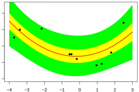
posterior is a four dimensional probability density function, therefore we depict it with a set of marginal posterior density plots. . . 63 3.5 The posterior predictive distribution for the quadratic model is

com-pared to the experimental data. The data are depicted with black points. The green interval is the 95% credibility interval of the pre-dictions. The yellow interval is the 50% credibility interval of the predictions. The red line is the median of the predictions. . . 64

(12)

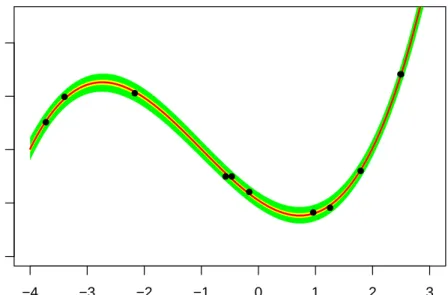
3.6 The posterior predictive distribution for the cubic model gives a better match to the data. The data are depicted with black points. The green interval is the 95% credibility interval of the predictions. The

yellow interval is the 50% credibility interval of the predictions. The

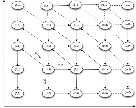
red line is the median of the predictions. . . 65 5.1 The CTMC that describes the LV model. States are labeled with the

number of prey and predators. Also, the transitions are associated with corresponding reactions. All the transitions represented with horizontal arrows will have the transition rate h1 = c1x1, the

tran-sitions represented with vertical arrows will have the transition rate

h3 = c3x2 and the transitions represented with diagonal arrows will

have the transition rate h2 =c2x1x2. . . 95

5.2 The figure shows the way in which the behaviour of the stochastic LV model can vary when the prey production reactionc1 ={0.6,0.1,0.8}

varies. . . 99 5.3 The figure shows the way in which the behaviour of the stochastic LV

model can vary when the prey production reactionc2 ={0.004,0.008,0.001}

varies. . . 100 5.4 The figure shows the way in which the behaviour of the stochastic LV

model can vary when the prey production reactionc3 ={0.8,0.5,0.2}

varies. . . 101 5.5 The figure illustrates several behaviours of the LV model, which are

simulated at different parameter values, as presented in Table 5.1. . 102 5.6 The figure shows the trace plot for each LV model parameter obtained

from the Gibbs sampler, where the Gibbs sampler applied to the synthetic data simulated at: (c1 = 0.1, c2 = 0.004, c3 = 0.15). The

(13)

List of Figures xi

5.7 The marginal posterior densities of the parameters of the LV model that are obtained by performing Gibbs algorithm is compared with the approximated marginal posteriors obtained from the ABC SMC with differentN using the synthetic data sets which are simulated at:

(c1 = 0.1, c2 = 0.004, c3 = 0.15) (top) and (c1 = 0.1, c2 = 0.002, c3 =

0.15) (bottom) respectively. The contour plots show the joint

den-sities which are estimated using a kernel density estimate (KDE). . . . 105 5.8 Approximation posterior distributions of the LV parameters obtained

from three individual runs (columns) of the ABC SMC using three different simulated data sets (rows). The prior distributions for each parameter are depicted by the green dashed line and the true pa-rameters are indicated by the red one. The approximate posterior distributions do not resemble the prior distributions, meaning that we are learning from the ABC SMC algorithm about those parame-ters. . . 106 5.9 The figure shows the ESS resulting from the performance of the

ABC SMC algorithm with differentN ={8000,4000,2000,1000,500} values respectively. The x axis represents the number of ABC SMC

stages. . . 107 5.10 The box plots illustrate the distribution of time across the

experi-ments running for each individual data set presented in Figure 5.5. It is obvious that the ABC SMC algorithms are cheaper than the Gibbs sampler. . . 108 5.11 The figure of box plots show the JSD divergence of the inferred LV

model parameters obtained from the Gibbs sampler and the ABC SMC algorithms with different settings of the target tolerance over

40 experiments. This figure indicates that the accuracy of the

ap-proximation increased as the target tolerance decreased. . . 111 5.12 Box plots show the total required computational time for the Gibbs

sampler and the ABC SMC algorithm across40experiments. The

re-sult indicates that the computational cost of the ABC SMC algorithm increased as the target tolerance decreased. . . 111 5.13 Target Tolerance estimation based on using different number of traces

(14)

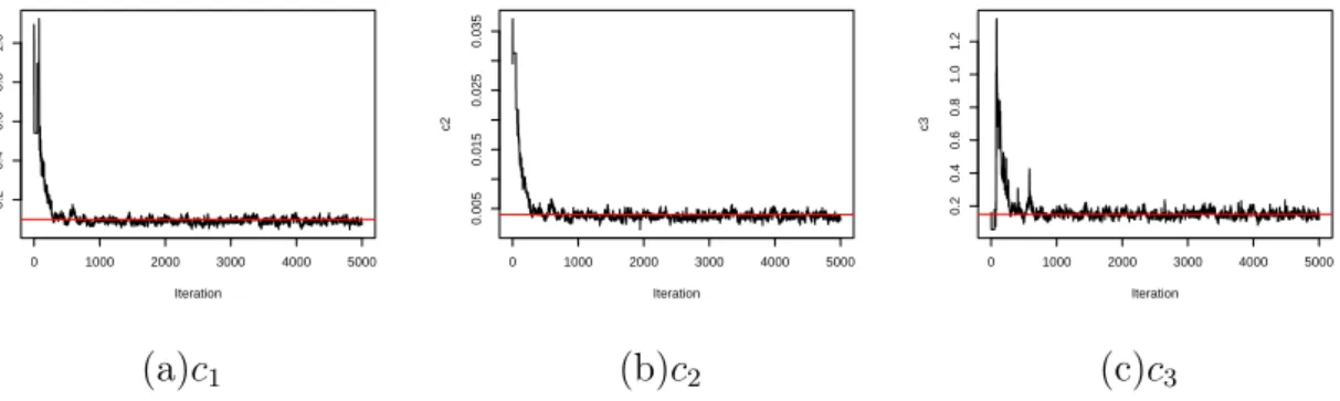
5.14 The figure shows the strong autocorrelation between samples for the LV model parameters. . . 114 5.15 The figure shows that all model parameters are converged to their

sta-tionary distributions as the resulting potential scale reduction (shrink factor) for all parameters are _Rˆ _≤₁_.₁_{. . . 115}

5.16 The posterior densities of the parameters of the LV model obtained from the PMMH1 (solid line) with its corresponding prior

distribu-tions (dashed line). The posteriors are three dimensional probability densities function. Therefore, we depict it with a set of marginal pos-terior densities. The contour plots show the joint densities which are estimated using a kernel density estimate (KDE). . . 116 5.17 The posterior densities of the parameters of the LV model obtained

from PMMH2 (solid line) with its corresponding prior distributions

(dashed line). The joint posterior densities are estimated using a kernel density estimate (KDE) and are depicted by contour plot. . . . 117 5.18 The figure shows the approximate posterior densities resulting from

applying the ABC SMC and the PMMH algorithms with its corre-sponding exact densities several times. Each column of this figure represents a specific model parameter that has been inferred, column one represents the posterior densities of c1, column two represents

the posterior densities ofc2 and column three represents the posterior

densities of c3. It can be seen that the estimate posterior

distribu-tions (resulting from PMMH1 and PMMH2) are distributed around

the exact posterior mode. The approximate posterior distributions are overdispersed and this is due to the ABC approximation where the quality of approximation depends on the level of the target toler-ance, but still, have similar support as the exact posterior densities.

. . . 119 5.19 Q-Q plots of the estimation of LV model parameters obtained from

the exact inference (black line) and approximate inference methods (ABC SMC, PMMH). The estimates shown in the first column are based on the ABC SMC and the second column are based on the PMMH algorithm. The first row represents the parameter c1, the

second row represents the parameter c2, and the third row represents

(15)

List of Figures xiii

5.20 The box plot displays the distribution of the resulting JSD divergence values over several independent runs of ABC SMC and both PMMH algorithms over different synthetic data sets (presented in Figure 5.1) which calculate the similarity between the approximate and the exact probability distributions for each LV model parameter. . . 121 5.21 Box plots of the exact posterior samples (blue box plot) which are

obtained from performing the Gibbs sampler versus the correspond-ing approximate distributions (green box plot) which are obtained from performing the ABC SMC with five settings of N, where the

term ABC500, ABC1000, ABC2000, ABC4000 and ABC8000 means

that the ABC SMC algorithm is performed with 500, 1000, 2000, 4000 and 8000 number of particles respectively. The term PMMH1

represent the performance of the PMMH algorithm with the normal proposal while the PMMH2 with log normal proposal density. It is

clear that the approximate posterior distributions resulting from the ABC SMC algorithm are widely distributed compared to the exact posterior distributions. While the resulting posterior distributions from both PMMH algorithms are tightly distributed around the ex-act posterior mode. . . 121 5.22 Accuracy of estimating the posterior density which is quantified through

the JSD divergence between the exact posterior distributions (Gibbs sampler) with its corresponding approximate posterior distributions versus the computational time for each algorithm across several runs. 124 5.23 The figure shows how the variance of the log likelihood estimator

obtained from the particle filter that is used in the PMMH algorithm to estimate the likelihood varies as the parameter values vary, where the true value in this example is 1(Wilkinson, 2011). . . 125

5.24 The resulting posterior densities from performing the PMMH1

al-gorithm two times with different tuning of the number of particles that used in particle filter algorithm to obtain the likelihood estima-tor. It can be seen that the posterior distributions obtained from the PMMH1 with N = 500 (red) are more similar to the exact posterior

densities than the original posterior densities (blue), in particular for parameter c3. . . 126

(16)

5.25 The resulting posterior distributions from applying the PMMH algo-rithm with a larger number of iterations in the burn in stage 3000

and stationary stage 5000 (red). It can be noticed that the tail of

the posterior distributions of the parameters c2 and c3 include more

parameter values compared to the original one (blue). . . 126 5.26 The resulting posterior distributions from combining 7 parallel runs

of the PMMH1 algorithm based on the normal proposal (blue) and 7 parallel runs of the PMMH2 algorithm based on the log normal

proposal (red). . . 127 5.27 Q-Q plots of the estimation of the LV model parameter obtained from

four PMMH algorithms and corresponding exact posteriors (Gibbs sampler). It is clear that the tails have not been fully explored by the PMMH algorithm. . . 127 5.28 The figure shows the approximate posterior densities for the LV model

parameters, the first row represents the inference given the data set presented in Figure 5.2 (a), the second row represents the inference given the data set presented in Figure 5.2 (b), the third row repre-sents the inference given the data set presented in Figure 5.2(c), and the fourth row represents the inference given the data set presented in Figure 5.4(a). Each column represents specific model parameter that has been inferred using the ABC SMC algorithm, column one represents the posterior densities of c1, column two represents the

posterior densities of c2, and column three represents the posterior

densities ofc3. . . 133

5.29 The plot represents the ESS values from performing the ABC SMC

algorithm, given the synthetic data set presented in Figure 5.2 (a). The ESS values for all runs have not dropped to very small value

(17)

List of Figures xv

5.30 The figure shows the approximate posterior densities which are re-sulting from applying the ABC SMC algorithm with three different choices of the adaptive tolerance schedule. The first row represents the inference given the data set presented in Figure 5.2 (a), the second row represents the inference given the data set presented in Figure 5.2 (b), the third row represents the inference given the data set presented in Figure 5.2(c). Each column represents specific model parameter that has been inferred using the ABC SMC algorithm, column one represents the posterior densities of c1, column two

rep-resents the posterior densities of c2, and column three represents the

posterior densities of c3. . . 135

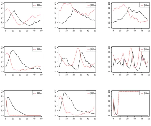
6.1 The original Repressilator network. . . 140 6.2 An illustration of the nine different synthetic data sets simulated from

the stochastic model using different parameter values. Only protein concentrations are plotted as differently coloured lines. mRNAs con-centrations were also simulated and used in inference, but they are omitted from these plots to avoid cluttering the visualisation. . . 143 6.3 The plot shows the ESS which is obtained from performing the SIS

algorithm on the first synthetic data set (Experiment1), the number

of SIS stages 35are represented in X-axis. . . 146

6.4 The distribution of model parameters (α, α0, n, β) at the first stage

of SIS sampler. All the particles at this stage are coming from the prior distribution. . . 147 6.5 The distribution of model parameters at one of the intermediate

stages (i = 19) of the SIS sampler. This distribution has already

diverged from the prior distribution, but it is still different to the posterior distribution. . . 148 6.6 The posterior distribution of the Repressilator model parameters (α, α0, n, β)

obtained using the SIS sampler. It is illustrated as a set of marginal posterior densities as the posterior defined in four dimensions. . . 149 6.7 The posterior distribution of the Repressilator model parameters

ob-tained using the ABC SMC algorithm. The dashed line represents the prior distribution. . . 151

(18)

6.8 The plot shows the ESS obtained from performing the ABC SMC

algorithm on the first synthetic data set (Experiment 1). . . 153

6.9 The distribution of model parameters at the first stage of ABC SMC algorithm. All the samples at this stage are coming from the prior distribution. . . 154 6.10 The distribution of model parameters at one of the intermediate

stages (i = 11) of ABC SMC algorithm. This distribution has slightly diverged from the prior distribution, but it is still different to the pos-terior distribution. . . 155 6.11 The posterior density of parameters of the Repressilator model given

the first synthetic data set, the dashed line represents the prior dis-tribution. . . 156 6.12 Approximate posterior distributions of the Repressilator model

pa-rameter obtained using ABC SMC giving a single synthetic data set. Dashed lines represent the sequence of distributions, solid lines show the final approximation posterior distributions, whereas the red ver-tical line shows the parameter values that have been used to simulate the synthetic data. . . 157 6.13 The plot represents theESS associates with experiment9 where the

ABC SMC applied with N = 8000, where X- axis represents the

number of ABC SMC stages25. . . 157

6.14 The plot represents theESScorresponding to several runs of experiment9,

in which ABC SMC applied with five differentN given the same

syn-thetic data. . . 158 6.15 Approximate posterior distributions of the Repressilator model

pa-rameters obtained from performing ABC SMC algorithm five times independently with different values of N, given the same synthetic

data set (Experiment 9). The five approximate posterior

distribu-tions are very similar. . . 158 6.16 The box plot represents the approximate posterior distributions of the

Repressilator model parameter obtained from performing ABC SMC

5 times independently with different values of N, giving the same

synthetic data set (Experiment 9). The five approximate posterior

(19)

List of Figures xvii

6.17 The box plot represents the approximate posterior distributions of the Repressilator model parameter obtained from repeating ABC SMC algorithm three times independently given the same synthetic data set. . . 159 6.18 The box plot shows the computational time for several runs of the

ABC SMC algorithm, given a different synthetic data sets that are depicted in Figure 6.2. It is obvious that the inference based on

N = 8000 requires more computational time compared to N = 500. . 160

6.19 The posterior density of parameters of the Repressilator model ob-tained from performing the PMMH, given the first synthetic data set, the dashed line represents the prior distribution. . . 161 6.20 The posterior density of parameters of the Repressilator model given

the first synthetic data set and the priors are shown in dashed line. . 162 6.21 The trace plot represents the chain after burn in period for the

Re-pressilator model parameter obtained from performing the PMMH algorithm using the first synthetic data set (Experiment 1). . . 163

6.22 The trace plot represents the chain after burn in period for the Re-pressilator model parameter obtained from repeating the PMMH al-gorithm (Experiment1). . . 163

6.23 The approximate posterior distributions for the Respressilator model parameter obtained from performing the ABC SMC and the PMMH given the synthetic data set generated at θ = {α = 1400, α0 =

1.5, n = 2, β = 0.2}. . . 164 6.24 The approximate posterior distributions for the Respressilator model

parameter obtained from performing the ABC SMC and the PMMH given the synthetic data set generated atθ={α= 1, α0 = 0.001, n =

2, β = 0.2}. . . 165 6.25 The approximate posterior distributions for the Repressilator model

parameter obtained from performing the PMMH. . . 165 6.26 The plot shows the GF protein concentration level for the

Repressi-lator model. . . 167 6.27 The sequence of tolerance values for each experiments. . . 168 6.28 The plot shows the ESS for each experiments. . . 169

(20)

6.29 Posterior distributions for the Repressilator model parameters ob-tained from performing the ABC SMC sampler, when M L= 200. . . 170

6.30 Posterior distributions for the Repressilator model parameters ob-tained from performing the ABC SMC sampler, when M L= 20. . . . 170

6.31 Posterior distributions for the Repressilator model parameters ob-tained from performing the ABC SMC sampler, when M L= 5. . . . 171

A.1 The marginal posterior density of parameters of the LV model which are obtained by performing the Gibbs algorithm compared with ap-proximated marginal posterior obtained from ABC SMC using the synthetic data set 3(diagonal plots). . . 179

A.2 The figure shows the marginal posterior density of parameters of the LV model which are obtained by performing the Gibbs algorithm compared with approximated marginal posterior obtained from ABC SMC using the synthetic data set 4 (diagonal plots). . . 180

A.3 The marginal posterior density of parameters of the LV model which are obtained from applying the Gibbs algorithm compared with ap-proximated marginal posterior obtained from ABC SMC using the synthetic data set 5(diagonal plots). . . 181

A.4 The marginal posterior density of parameters of the LV model which are obtained by performing the Gibbs algorithm compared with ap-proximated marginal posterior obtained from ABC SMC using the synthetic data set 6(diagonal plots). . . 182

C.1 The figure repressnts the marginal posterior density for the parameter of the LV model for5population size using data presented Figure 5.3,

resulting from performing ABC SMC algorithm. . . 186 C.2 The figure shows the marginal posterior density for the parameter of

the LV model for 5 population size using data presented Figure 5.4,

resulting from applying ABC SMC algorithm. . . 187 C.3 The figure represents the approximated posterior density resulting

from applying ABC SMC algorithm with three different quantile set-ting, the first row represent the inference given data set4, the second

row represents the inference given data set 5 and the third row

(21)

List of Figures xix

D.1 The figure shows the approximated posterior density for LV model parameter with its corresponding data set. . . 190 E.1 The posterior densities of the Repressilator model parameters

ob-tained from the PMMH sampler, given the synthetic data set gener-ated at parameter θ ={α= 1200, α0 = 1, n = 1, β = 3}. . . 192

E.2 The figure shows the posterior densities of the Repressilator model parameters obtained from performing the PMMH sampler, given the synthetic data set simulated with parameter θ = {α = 2400, α0 =

(22)

5.1 Computational time of the Gibbs sampler and the ABC SMC algorithm.104 5.2 The ESS obtained from various runs of PMMH1 and PMMH2. . . . 119

5.3 Summary of performing ABC SMC on synthetic data (presented in 5.2 (a)). . . 131 5.4 Summaries of the experiments of running the ABC SMC under a

dif-ferent tolerance schedules settings (based on three difdif-ferent quantiles). 132 6.1 Parameter settings for simulations from the Repressilator model. . . . 144 6.2 Summaries of total time for several runs. . . 164 B.1 Summaries of running the ABC SMC sampler. . . 184

(23)

List of Algorithms

1 CTMC Simulation algorithm . . . 25 2 Acceptance-Rejection Algorithm . . . 37 3 Self Normalised Importance Sampling (SNIS) Algorithm . . . 39 4 Sequential Importance Sampling Algorithm . . . 41 5 Sequential Importance Sampling Resampling . . . 44 6 Sequential Importance Sampling for state space model . . . 48 7 Metropolis-Hastings Algorithm . . . 53 8 Particle Marginal Metropolis-Hastings Algorithm . . . 68 9 Auxiliary variable Gibbs sampler for finite state Markov . . . 73 10 Perfect rejection sampling algorithm . . . 82 11 ABC rejection sampling algorithm . . . 83 12 Generalised ABC (GABC) . . . 84 13 ABC- SMC algorithm . . . 86 14 Forward-Backward algorithm . . . 178

(24)

Introduction

1.1 Introduction and Thesis Statement

This thesis considers the performance of Bayesian Inference of model parameters for Continuous Time Markov Chains (CTMC). CTMCs are a flexible class of stochastic models that consider a discrete state space with stochastic transitions in continuous time. These models have been widely applied in such fields as analysis of commu-nication protocols (Duflot et al., 2006), reliability analysis (Haverkort et al., 2000), power management (Qiu et al., 1999), and modelling biological systems (Calder et al., 2006).

A large part of the literature focusing on an analysis of CMTC considers the model to be completely observed. In more realistic situations, the problem of identifying model parameters to match the behaviour of the studied system is significantly more challenging (Milios et al., 2017).

When modelling a biological system, a set of ordinary differential equations (ODEs) is often used as a deterministic description of the system. These equations involve a concentration of species and parameters such as mRNA, protein, degradation and production rates. These equations provide an accurate description of the biological system when the number of molecules is large. Nevertheless, when the population of molecules is small, the impact of discrete stochastic behaviour is obvious, and the accuracy of this method becomes degraded (Schnoerr et al., 2017).

In addition, in practical studies in life sciences, it is difficult to observe every state and measure all parameters of the complex biological model. This motivates re-searchers to develop computational and mathematical approaches to help to

(25)

Chapter 1. Introduction 3

stand the systems’ mechanisms, behaviours and account for stochasticity. Moreover, a variety of inference methods have been proposed to quantify uncertainty relating to such systems.

Probabilistic Bayesian approaches have been used to quantify uncertainties in such systems, including work described in Golightly and Wilkinson (2005) and (Vyshemirsky and Girolami, 2008). Other studies have been considering using maximum likelihood estimation (Baker et al., 2005), (Timmer et al., 2004). When working with state space models, several sequential approaches have been proposed to handle state and parameter estimation problem such as particle filtering (Quach et al., 2007).

We consider the Bayesian approach to performing parameter inference because it allows quantifying uncertainties about inference results. Additionally, in cases when data provide little information for reliable parameter inference, for example, at the beginning of a new study, the Bayesian approach allows one to use pre-existing expert knowledge as an additional source of information via parameter prior distributions. The core problem of enabling parameter inference for state space models is the dif-ficulty in formulating the likelihood in a convenient form. Because the scale of the system grows, the likelihood function becomes intractable to evaluate. To cope with this, approximate methods can be applied that often rely on either variational infer-ence or simulation. Our primary focus in this thesis is on one particular approach that is based on statistical simulation.

This thesis does not intend to provide a complete overview of other inference ap-proaches for CTMC models, but we will briefly mention some of them. A recent review included the theory and inference methods for a Markov process in a biolog-ical modelling context (Schnoerr et al., 2017).

The work presented in this thesis approaches the problem of Bayesian parameter inference using approximate inference methods that avoid direct evaluation of the likelihood. Simulation from the model is used instead to approximate the likeli-hood via an unbiased estimator based on Monte Carlo integration. We consider two general sampling schemes that implement this approach in two slightly differ-ent forms. The Particle Marginal Metropolis Hastings sampler (Wilkinson, 2011) performs likelihood estimation using a simulation based particle filter, while the Ap-proximate Bayesian Computation with Sequential Monte Carlo (ABC SMC) (Sisson et al., 2007a), (Peters et al., 2012) sampler relies on repeated resampling of a parti-cle population along a sequence of gradually improving approximating distributions. A pseudo-marginal sampler based on truncation is new to the statistics field and

(26)

provided exact inference for such systems (Georgoulas et al., 2017). We employ this method as a reference for our case study.

We implement these sampling schemes, study their properties and tuning parame-ters, and perform a comparison of their performance in two complex case studies. The accuracy of the results obtained from these approaches is verified by comparison to the exact method.

1.2 Thesis Contribution

In this thesis, we demonstrate that CTMC can be applied to modelling complex stochastic systems. Uncertainty quantification for those stochastic systems is stud-ied. In particular, parameter estimation with tuning algorithmic parameters demon-strates how these methods work in practice.

We provide two extensive studies where CTMC are used to model molecular reaction networks in biology. The main contributions of this thesis can be summarised as:

• We give an up-to-date review of the state-of-the-art methods for Bayesian inference without explicit likelihood.

• We study such methods in detail and discuss the tuning of these algorithms. Specifically, the choice of the number of particles in the particle filter, selection of the optimal proposal distribution and convergence diagnostics in the Particle Marginal Metropolis Hastings sampler are studies to improve the exploration of the parameter space and hence the efficiency of the algorithm.

• An extensive comparison between the exact inference approach and approxi-mation approaches involving the accuracy, complexity of the implementation and computational costs was performed.

• We evaluate these methods by making inference for a challenging stochastic model with intractable likelihood. We utilise the Particle Marginal Metropo-lis Hastings sampler and Approximate Bayesian Computation on the Lotka Volterra model. Moreover, we resort to the recently developed exact method, which is known as a Gibbs sampler based on truncation to quantify the accu-racy of approximation methods.

• Motivated by the high variability of the system behaviour, the Repressilator system is chosen to utilise the proposed inference methods involving both

(27)

Chapter 1. Introduction 5

synthetic and real data.

1.3 Outline of the Thesis

This thesis is divided into seven chapters. A brief overview of each chapter and a description of the general thesis structure is given below.

In Chapter 2: We provide the reader with an overview of Markov processes,

covering the main concepts and definitions. We also introduce the Continuous Time Markov Chain models relevant to this study and define how CTMC can be used to model biochemical reaction systems.

In Chapter 3: We consider the Bayesian inference framework and also discuss the

main issues to deal with when working within this framework. A general review of Monte Carlo methods is given. Possible inference problems, such as the intractability of the likelihood term, are illustrated.

In Chapter 4: We describe the Approximate Bayesian Computation scheme,

in-troduce the ABC SMC sampler, and discuss tuning parameters for this method.

In Chapter 5: We consider the first case study concerning modelling of the

stochas-tic Lotka-Volterra system, perform parameter inference for this case study using approximate sampling algorithms, and compare them to the exact method.

In Chapter 6: We consider the second case study concerning a more complex

biochemical system known as the Repressilator (Elowitz and Leibler, 2000). First, we investigate how the algorithm tuning parameters impact the inference results. Then we perform a validation study using a real data set.

In Chapter 7: We review and discuss the results obtained in this work. Possible

(28)

Markov Chains

Most natural phenomena are difficult to observe directly. Statistical models, on the other hand, can be used to understand and predict the behaviour of such systems. Often, these phenomena involve randomness, which can be quantified through prob-ability theory. A random phenomenon can be described by evaluation of a random variable in time. Numerous probabilistic models are applied to explain the system’s behaviour. Some stochastic processes have a memoryless property, meaning that the future state of the system can rely only on its present state, independent of its whole past history. Such a stochastic process having a memoryless property was in-troduced and studied by a Russian mathematician, Andrey Markov. This stochastic process is called a Markov process. Markov processes can be classified based on their timing and state. The main types of the Markov process are a discrete time Markov Chain (DTMC) and a continuous time Markov Chain (CTMC) (Bhattacharya and Waymire, 2009). There are several applications of Markov chains in various scien-tific fields. In this thesis, in an attempt to understand the Markov chain, we begin with a brief introduction to the Markov process, covering the basic concepts, giving a definition, and describing the theorems and essential properties. We continue this chapter by considering a DTMC, its structure and main properties, where a DTMC is characterised by a discrete state and time, which are assumed to be homogeneous (see section 2.2). In addition, essential features of the Markov chain necessary for studying the chain’s long term behaviour are discussed and explained. A CTMC will also be considered in detail as it serves as the main practical model in this thesis (Norris, 1998), (Ross, 2014).

(29)

Chapter 2. Markov Chains 7

2.1 Stochastic Process

A stochastic process is a vector of random variables, which can be indexed by discrete nonnegative integer e.g. {X1, X2,· · · } or {Xt : t∈N}. The state of the system at

discrete timetis denoted asXtand takes values in a countable and finite state space

X. The random variable can also be indexed by continuous time e.g{X(t) :t∈R}.

2.2 Markov Chains in a Discrete State Space

Definition 2.2.1. (Markov Chain)

A stochastic process {Xt:t∈N} is defined as a discrete time Markov chain if it

satisfies the Markov property:

P (Xt+1 =j|X0 =x0,· · · , Xt =i) = P(Xt+1 =j|Xt=i),

where i, j, x0,· · · , xt−1 ∈ X and t∈N.

The previous equation means that the whole past history before state Xt has been

forgotten, which is known as the memoryless property. Thus, the conditional prob-ability of state Xt+1 is independent of all past states X0, X1,· · · , Xt and depends

only on the current state Xt. A process with such properties is referred to as a

Markov process and is commonly called a Markov chain.

Definition 2.2.2. (Homogeneous Markov chain)

A homogeneous Markov chain can be described as a conditional probability that does not depend on the current time,

∀m ∈N:P(Xt+m =j|Xt+m−1 =i) =P(Xt =j|Xt−1 =i).

P(Xt+1 =j|Xt =i)is the probability of the process moving from stateito the next

state j in a unit time and is known as a one-step transition probability, denoted as: pij.

For a homogeneous DTMC, let us assume that there is a probability governing the transition between the states, denoted aspij. Thus, a one-step transition probability

(30)

P(Xt+1 =j|Xt=i) =pij, where i, j = 1,2,3,· · · . (2.1)

All possible transition probabilities pij can be defined as matrix P.

2.2.1 Transition Matrix

The transition probability pij is interpreted as the probability that the process can

change randomly from one state to another one, and it can be presented as a matrix.

Definition 2.2.3. (Probability transition matrix)

Given the fact that a state space X contains N states, the transition matrix is

defined as an N ×N matrix with nonnegative entries, where all rows add up to 1,

denoted as P: P=        p11 · · · p1N p21 · · · p2N ... ... ... pN1 · · · pN N        ,

where the ith row of the transition matrix Prepresents the probabilities of moving

out from state i to another state. The column j of P expresses the transition

probability into state j.

2.2.2 Chapman-Kolmogorov Equation

A 1-step transition probability pij was defined in 2.1. However, in order to

under-stand the path of transition in a Markov chain, it is useful to describe the probability of jumping from state i to another state j in m steps, making use of intermediate

states. To illustrate this, we begin with a simple case when m = 2, so the

proba-bility of transition between states iand j can be calculated in two steps via a third

(31)

p2_ij =P(X2 =j|X0 =i)

=X

r

P(X2 =j, X1 =r|X0 =i) By law of total probability

=X r P(X2 =j|X1 =r, X0 =i)P(X1 =r|X0 =i) By product rule =X r P(X2 =j|X1 =r)P(X1 =r|X0 =i) By Markov property =X r prjpir =X r pirprj. (2.2)

This can be generalised to compute a m-step transition probability as:

pm_ij =X

r

pm_ir−1prj. (2.3)

These are known as the Chapman-Kolmogorov equations that are used to compute the probabilities, implying that the process arrives into a specific state after msteps

through intermediate steps.

Theorem 2.2.1. (The Chapman-Kolmogorov equations)

In a finite DTMC, given the two states iat time 0and j at time m+t with timem

and t, the transition probability between the states is given as:

pm_ij+t=X

r

pm_irpt_rj.

Proof. In order to prove the Chapman-Kolmogorov equations, we use the law of

total probability, the product rule and the Markov property, which results in the following:

(32)

The Chapman-Kolmogorov equations can be defined in a matrix form e.g. P·P=P2

which is equivalent to p2

ij =

P

rpirprj. In a more general way, the

Chapman-Kolmogorov equations can be written in a matrix form as:

Pm+t=Pm·Pt.

2.3 State Probabilities

We have already considered the conditional probabilities of transition between states. In this section, we aim at considering the unconditional probability of any state at a given time n. It is important to begin by defining the probability of the initial

state.

Definition 2.3.1. (Initial distribution)

For a time-homogeneous Markov chain {Xt}, the probability distribution of the

initial state at time 0 is defined as:

∀i∈ X :π0_i =P(X0 =i),

where

X

i∈X

π_i0 = 1.

The definition of the probability of the initial state is necessary in the evaluation of the unconditional probability for the state. Suppose we want to compute the following unconditional probability:

(33)

Chapter 2. Markov Chains 11 πt_j =P(Xt=j) = N X i=1 P(Xt=j, X0 =i) = N X i=1 P(Xt=j|X0 =i)P(X0 =i) = N X i=1 pt_ijπ_i0,

where P(Xt = j|X0 = i) = pijt and P(X0 = i) = πi0 then, the t-step transition

matrix can be built as:

Pt=        pt 11 · · · pt1N pt 21 · · · pt2N ... ... ... pt_N₁ · · · pt_{N N}        .

Let us consider the simplest case when t = 0 and t= 1, then:

p0_ij =P(X0 =j|X0 =i) =    1 if i=j 0 if i6=j

which means that: P0 =I. In the case of t= 1, we have:

p1_ij =P(X1 =j|X0 =i) =pij.

and hence P1 =P.

The state probabilities in t-steps can be calculated as:

π1 =π0P

π2 =π1P=π0P2

π3 =π2P=π0P3.

The above equations can be generalised as:

(34)

where πt is the row vector containingπ_jt, wherej = 1,· · · , N.

A DTMC can be identified by two main components: the initial distribution and the transition probability.

2.3.1 Important Properties and Classification of States in a

Markov Chain

In this section, in the context of a discrete state Markov chain, the essential prop-erties are briefly introduced. In addition, we will list the classification of Markov chains according to the transition probabilities. As a rule, a Markov chain converges to a stationary distribution. In order to reach this stationary distribution, the chain must satisfy certain conditions such as irreducibility and aperiodicity. These prop-erties are required to ensure that a Markov chain visits any region of the state space at any unit of time. We begin with a definition of these properties.

Definition 2.3.2. (Accessibility)

Letiand j be two states in a discrete state space Markov chain. It can be said that

state j is reachable or accessible from state i, denoted asi→j if:

inf{t:P(Xt =j|X0 =i)>0}<∞,

or, in other words, it can be expressed through the transition probability matrix as

inf{t:pt_ij >0}<∞.

This definition can be used to introduce another concept, known as Communication, which considers the relationship between states.

Definition 2.3.3. (Communication)

It can be said that states i and j are communicating if each is reachable from the

other. This can be written in the form:

i↔j iff i→j and j →i.

This property allows us to define the important concept of irreducibility:

Definition 2.3.4. (Irreducibility)

A Markov chain is irreducible if all states are communicating with each other in that way: ∀i, j ∈ X :i↔j.

(35)

Definition 2.3.5. (Periodicity)

Given a stateiin a DTMC, the period of statei, denoted asdi, is defined as follows:

di =gcd{t≥1 :ptii>0},

where gcd represents the greatest common divisor. The state is named periodic if

di >1, otherwise, if di = 1 it is aperiodic.

Another important concept needs to be studied to understand the behaviour of the Markov chain states, and this is based on the number of visits to a particular state if a Markov chain runs infinitely.

2.3.2 Recurrence and Transience

In a chain, there are states that will be visited several times and sometimes others infinitely. To illustrate this concept, let us define the following:

ηi(t) =    1 if Xt =i 0 if Xt 6=i.

We can define the number of visits to a state i by Vi = P

∞

t=0ηi(t). The expected

number of visits ( given that the chain in state i) is:

E(Vi) = ∞ X t=0 E(ηi(t)) = ∞ X t=0 P(Xt =i|X0 =i) = ∞ X t=0 pt_ii.

The expected number of visits to a state will be used to classify the state as recurrent or transient.

Definition 2.3.6. (Recurrence)

The state i in a DTMC is recurrent if P∞

t=0p

t

ii = ∞, otherwise, the state is called

transient if P∞

t=0ptii <∞.

Let us assume that the initial passing time to return to state i is presented as:

Ti = inf{t >1;Xt=i}.

(36)

In a DTMC, if the state i is recurrent, then, i can be considered as a positive

recurrent if:

E(Ti|X0 =i)<∞.

Definition 2.3.8. (Null Recurrent)

In a DTMC, if the state iis recurrent, then, it can be considered as a null recurrent

if:

E(Ti|X0 =i) = ∞.

Definition 2.3.9. (Ergodic)

An irreducible DTMC can be considered ergodic if all states are positive recurrent and aperiodic.

A proof is given by (Gilks et al., 1995). We have considered a Markov chain and its properties. In the light of these properties, an important concept will be discussed in the following section. This is the invariant or the so called stationary distribution, which is often utilised in a Markov chain as Monte Carlo methods to build a sample targeting a particular distribution.

Definition 2.3.10. In an irreducible, ergodic DTMC, the limiting distribution

ex-ists and can be defined as follows :

πj = lim t→∞p

t

ij, ∀i∈ X,

where πj is the unique solution of:

πj = N X i=0 πipij, N X j=0 πj = 1.

Definition 2.3.11. Given a DTMC with a transition matrix P=pij,where i, j ∈

X. A distribution πj can be considered as a stationary distribution or invariant

distribution of a Markov chain (Xt, t≥0)if the following is satisfied:

πj = N

X

i=1

(37)

In order to ensure that a Markov chain has a stationary distribution, a specific condition must be met. This condition is known as a detailed balance equation. This type of Markov chain also exhibits reversibility and is known as a reversible Markov chain.

2.3.3 Time Reversible Markov Chain

Let us suppose that an ergodic Markov chain exists with the transition probabilityp0_ij

and the stationary distribution πj. Let us further assume that the state is moving

backwards so that a sequence of states Xt+1, Xt, Xt−1, . . . is in the reverse order,

which means the distribution of Xt is conditional rather on the future than on the

past. Hence, the transition probability can be written as:

p0_ij =P(Xt=j|Xt+1=i) = P(Xt=j, Xt+1 =i) p(Xt+1 =i) = P(Xt+1=i|Xt=j)p(Xt=j) p(Xt+1 =i) =pji πj πi .

Then, a time reversed Markov chain is considered as a Markov chain with:

p0_ij =pji

πj

πi

.

Definition 2.3.12. (Reversibility) A Markov chain is called reversible if it satisfies

the condition:

πipij =πjpji ∀i, j ∈ X.

This condition is also called the detailed balance equation, where for both states i

and j, the movement from i and j occurs at the rate πipij. It is exactly similar to

the transition rate from j and i, which is πjpji.

More details about a DTMC and its properties, theorems, proofs and definitions can be found in (Chung, 1967), (Kemeny et al., 1960) and (Karlin and Taylor, 1981). A discrete time Markov chain has been widely used to model different phenomena. A DTMC also plays a key role in the Metropolis-Hastings class of the sampling

(38)

al-gorithm considered in this thesis. However, most real phenomena rely on continuous time, while a DTMC is limited to discrete time. This motivates us to consider a Markov chain with continuous time.

2.4 Continuous Time Markov Chains

In this section, we provide details of other important type of a Markov chain, namely, the continuous time Markov chain (CTMC) with its essential properties. We have already described the main concepts of a DTMC when properties of a Markov chain and the classification of states have been investigated. We will now investigate a CTMC. A CTMC can be distinguished from a DTMC by the state index t, which

is a real number t ∈ R. In addition, in CTMC, the notations are slightly different

from DTMC, the transient probabilities matrix will be P(t)instead of Pt, the state

probability in DTMC is assumed to beπt

i =P(Xt=i)while in CTMC is presented

as: πi(t) =P(X(t) = i).

A continuous-time stochastic process {X(t) :t≥0} can be considered as a Markov process when the future state relies only on the current state and is independent from all history.

Definition 2.4.1. (CTMC)

The tuple (X, xinit,Q)is CTMC where:

• state spaceX is a finite set of states. • The initial statexinit ∈ X.

• The transition rate matrix isQ:X × X →qij≥0.

In a CTMC, the transition between states is governed by the rate matrixQfor each

pair i and j. A transition from state i to state j can occur when the matrix index

is qij >0.

The transition probabilities and state waiting are determined by the matrix Q.

Assume that the exit rate of state i is given as E(i) =P

j∈X,j6=iqij, then, the mean

of the waiting time (which follows an exponential distribution ) for state i is _E1₍_i₎.

The probability of transition from state i occurring within time t is given as 1−

e−E(i)·t. The probability that the transition fires from state i to state j is qij

(39)

the transition rate is qij = 0, this implies there is no transition from i to j. This

matrix is known as the generator matrix Q and can be defined as:

Definition 2.4.2. (Generator matrix)

Let us assume that the generator matrix associated with a CTMC is denoted by Q,

then off diagonal entries are presented asqij and the diagonal entries areqii=−E(i).

The generator matrix satisfies the following: • 0≤ −qii<∞ ∀i.

• qij ≥0 ∀i6=j.

• P

jqij = 0.

A CTMC follows the same property of a DMTC. For instance, a state j is accessible

or reachable i if qij ≥0.

Let us assume that we have a CTMC with N states, when the transient state

probability is defined:

π = (π0(t), π1(t),· · ·, πN(t)),

where the probability of a CTMC being in particular stateiat unit timet isπi(t) =

P(X(t) = i). The dynamics of a CTMC are described by:

d

dtπ =πQ.

The Chapman-Kolmogorov equation can be expressed in the matrix form as:

d

dtP(t) = P(t)Q.

where P(t) represents the transition matrix that is defined in section 2.2.1.

The stationary behaviour can be obtained via solving the following system of equa-tions: πQ= 0, N X i=1 πi = 1.

(40)

Solving this equation requires a CTMC to be irreducible and finite. In this thesis, we focus on transient probability, while reader interested in stationary behaviour is referred to (Drake, 1967), (Cox, 2017).

2.5 An Overview of Modelling Biological Systems

Stochasticity exists in most biological systems. A biological process can involve randomness due to the random collisions and interactions between different system components such as molecules inside cells. Stochastic chemical kinetics provides a description of the dynamic behaviour of such networks and account for stochasticity, the randomness of which has a significant influence on the behaviour of the model (McQuarrie, 1967), (Zheng and Ross, 1991).

A reaction network can be defined as a chemical reaction system including several species and reactions. Each reaction in the system occurs at a stochastic rate which implies that a stochastic model is needed. The reaction systems are modelled as a discrete state representing the number of molecules of species over continuous time resulting in a CTMC. A CTMC enables us to evaluate a biochemical process and its uncertainty over time by estimating the probability of the system being in a specific state at a given time. The probability that the system is at a certain state through certain time can be determined by the Chapman-Kolmogorov equations also known as the Chemical Master Equation (CME). However, the state space of a CTMC increases exponentially in terms of the number of molecules, which results in a large state space of a CTMC. Thus, solving the CME analytically or numerically turns out to be a difficult task (Munsky and Khammash, 2006).

Instead of determining the probability distribution over the various states of the system at each time by solving this equation, a sample can be drawn from their distribution. The generation of a sample trajectory is straightforward due to the proposed stochastic simulation algorithm (Doob and Doob, 1953). The advantage of using simulation of a stochastic model is about having simpler performance. More-over, many sample paths can be simulated despite the size of the state space of a CTMC. Several exact and approximate methods have been proposed in the literature to solve the CME, we review some of these methods briefly in section 2.6.

(41)

2.5.1 Stochastic Biochemical Kinetic

A brief description of the stochastic behaviour and the function of a biological system through a biochemical reaction network using a Markov process will be given in this section (Gillespie, 1991), (Gillespie, 1996), (Wilkinson, 2011).

Consider a constant reaction volume Ω, which is assumed to be well-stirred and

in thermal equilibrium. A collision between molecules can occur randomly which consequently results in a specific reaction. To illustrate these reactions, consider N

different species denoted as (X1,· · · , XN) with their N populations which can be

the number of molecules of species, denoted as (x1,· · · , xN).

A biochemical reaction between two distinct speciesXi and Xj can be unimolecular

or bimolecular reactions. This can occur if they collide while they are moving randomly and produce another species, as follows:

1. A bimolecular reaction can occur between any two distinct types of speciesXi

and Xj is presented as:

Xi+Xj ci

−→P roducts.

2. A n unimolecular reaction is when a molecule of the species Xi is transferred

to a molecule of another species like that:

Xi ci

−→P roducts.

3. An unimolecular reaction: a production and degradation of a chemical species can be presented, respectively, as:

∅ ci

−→P roducts.

Xi ci

−→ ∅,

where ∅ in the previous equation refers to a species which are not considered in the system. Now, a biochemical reactions system will be described in terms of a Markov process.

Each reaction occurs with a specific constant kinetic ratec1, . . . , ci and is associated

with the hazard function, sometimes called the stochastic rate law which will be defined as follows:

(42)

Definition 2.5.1. (Hazard function)

Hazard function, denoted by h(t)dt, is the conditional probability that a specific

type of reaction takes place in the infinitesimal interval (t, t+dt], given that this

reaction has not occurred at time t:

h(t)dt=P(t < T ≤t+dt|T > t),

whereT is a nonnegative random variable representing the time of occurrence of the

reaction (Steward, 2009).

As described in (Wilkinson, 2011), the hazard function relies only on the reactant population X = (x1,· · · , xn) and a constant rate ci. In the case of unimolecular

reaction or zero order reaction, the hazard function is the constant rate of the reaction:

hi(x, ci) = ci.

While in a first order reaction, only one molecule xi of species Xi is required for a

reaction to take place, and, the hazard function is:

hi(x, ci) =ci.xi.

For a reaction of the second order, two distinct moleculesxdandxj from two different

species Xd and Xj are required, and the total combination of xj·xd with constant

rate ci can form the hazard function:

hi(x, ci) =ci·xj·xd.

2.5.2 The Markov Description of Biochemical Reaction

Net-work

Consider a well-mixed system of N species, with populations (X1,· · · , XN). This

population can interact with distinct species and result in L reactions, denoted

by (R1,· · · , RL) which can be expressed using either unimolecular or bimolecular

reactions. The most widely used method to represent a biochemical network is a set of chemical reaction equations which take the form of (Wilkinson, 2011):

(43)

Chapter 2. Markov Chains 21 R1 :p11X1+p12X2+· · ·+p1NXN c1 −→q11X1+q12X2+· · ·+q1NXN R2 :p21X1+p22X2+· · ·+p2NXN c2 −→q21X1+q22X2+· · ·+q2NXN ... RL:pL1X1+pL2X2· · ·+pLNXN cL −→qL1X1+qL2X2+· · ·+qLNXN, (2.4)

where the reactants pij and the products qij ∈ N0 are known as the stoichiometric

coefficients.

It can be presented in a matrix form P X →QX, where the entire pij and qij, the

stoichiometric coefficients, form this matrix.

This matrix specifies the number of consumed and produced molecules in each species based on the occurrence of the reaction. When reaction i,where i = 0,· · · , L fires, the number of molecules of xj,where j = 0,· · · , N can decrease

by pij and increase by qij, then the overall change will be vij =pij −qij.

The reactionRiis described as the stochastic vectorvij that represents the molecules

population after a reaction occurs. The second important quantity that characterises the system is the hazard function, where, a set of chemical reactions Ri takes place

at specific hazard rate constants c1, . . . , ci and hazard function hi and this process

is known as chemical kinetics (Gillespie, 2007).

In a stochastic framework, a random location of the reaction is considered, and thus the number of molecules in each space is a random variable. Consequently, the hazard function hi is also a random variable.

As we are working with a probabilistic mathematical model, let us assume that the system is characterised by a set of time dependent states vectorx= (x1(1),· · · , xN(t))T

which represents the molecular number of each species (X1,· · · , XN)at given time

t. For instance, if the system is currently at state x and whenever a reaction Ri

takes place, then the system state jumps to another state x+vi. Since we assume

that the system is well mixed meaning that the diffusion and locations of molecules are not modelled, continuous-time Markov chains (CTMC) can be used to model the dynamics of the system.

In particular, the biochemical reaction can take place randomly, resulting in the change of the molecules count and hence lead to a discrete state space X(t)Markov

chain with a continuous time (CTMC) (Anderson and Kurtz, 2011), (Gillespie, 1992), (Gardiner, 1986).

(44)

A CTMC is defined as the integer-valued state path describing the transition be-tween the state if a reaction fires. The transitions of a CTMC are identified by the probabilities of occurrence of distinct reactions with the infinitesimal interval

(t, t+dt]. Let now describe the probability of the possible transition of a CTMC

according to the distinct reaction occurring such way:

1. If the system is in state Xt = x, the probabilities of occurrence of particular

reaction Ri within a infinitesimal time interval (t, t+dt] are given as:

P(X(t+dt) = x+vi|X(t) =x) = hi(x, ci)dt+O(dt),

where hi(x, ci) = ci·x is the hazard function and the term O(_dtdt) goes to zero

as dt→0.

2. The probability that the system remains in the current state and no more reactions take place is:

P(X(t+dt) =x|X(t) = x) = 1−

L

X

i=1

hi(x, ci)dt+O(dt).

3. The probability that multiple reactions will occur in an infinitesimal interval

(t, t+dt]is O(dt).

The kinetic law of the system can be obtained through the evaluation of the sys-tem’s probability. The Chemical Master Equation can provide an evaluation of the system’s probability distribution (Van Kampen, 1992).

2.5.3 The Chemical Master Equation

In this section we are aim at evaluating the stochastic reaction network via comput-ing the probabilities of states at any particular time t. Let us assume that we are

interested in computing the probability of the system being in statexat a particular

time t, given the fact that the system was in a state x0 at time t = 0. The

proba-bility P(X(t+dt) = x|X(0) =x0)after a period of timedt can be decomposed into

(45)

Chapter 2. Markov Chains 23 P(X(t+dt) = x|X(0) = x0) = L X i=1 hi(x−vi, ci)dt+O(dt) P(X(t) =x−vi|X(0) = x0) + 1− L X i=1 hi(x, ci)dt+O(dt) P(X(t) =x|X(0) =x0).

The first term represents the probability that one reaction fires in the time interval

[t, t+dt] multiplied by the probability that the system is jumping from x to state x − vi. The second term is the probability that the system remains in a state

x multiplied by the probability that no reactions take place in the time interval

[t, t+dt].

To obtain the CME, subtracting P(X(t) = x|X(0) = x0), taking the limit limdt→0

and dividing by dt, we get:

For simplicity, we will assume that P(X(t) =x|X(t0) = x0) =Pt(x), then the CME

can be rewritten as follows:

d dtPt(x) = L X i=1 hi(x−vi, ci)Pt(x−vi)− L X i=1 hi(x, ci)Pt(x). (2.5)

The equation (2.5) is a coupled system of linear ordinary differential equations. In a Markov framework, the previous equation is commonly known as the Kolmogorov’s forward equation that is used to evaluate the probability of a transition between states (Gillespie, 1992),(Gardiner and Zoller, 2004) and (Gardiner, 1986).

(46)

CMEs have mostly been used for modelling stochastic biological systems and gen-erally are difficult to solve. A distribution Pt(x)is known as a steady state solution

of the equation 2.5 if it satisfies the condition d

dtPt(x) = 0.

However, despite the simplicity of this system, computing CMEs is often intractable because the state space size increases once the number of molecules in each species grows. This consequently leads to a large number of ordinary differential equations. Therefore, the analytical solution of the CME is available only for some specific cases (Munsky and Khammash, 2006). Hence, different approaches have been considered in the literature to approximate the CME, and they are described briefly in the section (2.6). In addition, a stochastic simulation can be used to study the behaviour of such a biological system.

2.5.4 Stochastic Simulation

A stochastic simulation algorithm provides a way to sample exact realisation X(t)

of the stochastic system defined by the CME. A stochastic simulation was initially suggested by Gillespie (1976) in the chemical kinetics context, and then different variants were proposed in the literature (Mauch and Stalzer, 2011).

The algorithm simulates a stochastic reaction system as a CTMC which consists of discrete states with continuous time based on drawing an exponential waiting times for all reactions and selecting the smallest waiting time for the next reaction. A standard and widely used approach to simulate such stochastic reaction systems is the Gillespie’s algorithm (Doob and Doob, 1953), (Gillespie, 2007), described below:

2.6 Related Works

The first part of this section provides a brief review of existing classes of the system that can be evaluated analytically, and in the second part of this section; some of an existing approximation methods in the literature reviewed.

2.6.1 Exact Methods

The analytic solution to the CME is known only for a restrictive class of systems and few simple special cases. In practice, it is difficult to derive an exact solution for many systems of interest. However, a stochastic simulation algorithm can be used