1 doi: 10.1093/bib/bbaa167
Method Review
Large-scale benchmark study of survival prediction
methods using multi-omics data
Moritz Herrmann, Philipp Probst, Roman Hornung, Vindi Jurinovic and
Anne-Laure Boulesteix
Corresponding author: Moritz Herrmann, Department of Statistics, Ludwig Maximilian University, Munich, 80539, Germany. Tel: +49 89 2180 3198; E-mail: [email protected].
Abstract
Multi-omics data, that is, datasets containing different types of high-dimensional molecular variables, are increasingly often generated for the investigation of various diseases. Nevertheless, questions remain regarding the usefulness of multi-omics data for the prediction of disease outcomes such as survival time. It is also unclear which methods are most appropriate to derive such prediction models. We aim to give some answers to these questions through a large-scale benchmark study using real data. Different prediction methods from machine learning and statistics were applied on 18 multi-omics cancer datasets (35 to 1000 observations, up to 100 000 variables) from the database ‘The Cancer Genome Atlas’ (TCGA). The considered outcome was the (censored) survival time. Eleven methods based on boosting, penalized regression and random forest were compared, comprising both methods that do and that do not take the group structure of the omics variables into account. The Kaplan–Meier estimate and a Cox model using only clinical variables were used as reference methods. The methods were compared using several repetitions of 5-fold cross-validation. Uno’s C-index and the integrated Brier score served as performance metrics. The results indicate that methods taking into account the multi-omics structure have a slightly better prediction performance. Taking this structure into account can protect the predictive information in
low-dimensional groups—especially clinical variables—from not being exploited during prediction. Moreover, only the block forest method outperformed the Cox model on average, and only slightly. This indicates, as a by-product of our study, that in the considered TCGA studies the utility of multi-omics data for prediction purposes was limited.
Contact:[email protected],+49 89 2180 3198
Supplementary information:Supplementary data are available atBriefings in Bioinformaticsonline. All analyses are reproducible using R code freely available onGithub.
Key words: multi-omics data; prediction models; benchmark; survival analysis; machine learning; statistics
Moritz Herrmannis a PhD student at the department of statistics, University of Munich (Germany). His research interests include computational statistics, machine learning and functional data analysis.
Philipp Probstobtained a PhD in statistics from the University of Munich, working at the Institute for Medical Informatics, Biometry and Epidemiology (Germany). His research interests include machine learning, statistical software development and benchmark experiments.
Roman Hornungis a postdoctoral fellow at the Institute for Medical Informatics, Biometry and Epidemiology, University of Munich (Germany). His research interests include biostatistics, computational statistics and machine learning.
Vindi Jurinovicis a postdoctoral fellow at the Institute for Medical Informatics, Biometry and Epidemiology, University of Munich (Germany). Her research interests include biometry, bioinformatics and computational molecular medicine.
Anne-Laure Boulesteixis an associate professor at the Institute for Medical Information Processing, Biometry and Epidemiology, University of Munich (Germany). Her activities mainly focus on computational statistics, biostatistics and research on research methodology.
Submitted:7 March 2020;Received (in revised form):25 June 2020
© The Author(s) 2020. Published by Oxford University Press. All rights reserved. For Permissions, please email: [email protected]
This is an Open Access article distributed under the terms of the Creative Commons Attribution Non-Commercial License (http://creativecommons.org/
licenses/by-nc/4.0/), which permits non-commercial re-use, distribution, and reproduction in any medium, provided the original work is properly cited. For commercial re-use, please contact [email protected]
Introduction
In the past two decades, high-throughput technologies have made data stemming from molecular processes available on a large scale (‘omics data’) and for many patients. Starting from the analysis of whole genomes, other molecular entities such as mRNA or peptides have also come into focus with the advancing technologies. Thus, various types of omics variables are currently under investigation across several disciplines such as genomics, epigenomics, transcriptomics, proteomics, metabolomics and microbiomics [1].
It may be beneficial to include these different data types in models predicting outcomes, such as the survival time of patients. Until recently, only data from a single omics type were used to build such prediction models, with or without the inclu-sion of standard clinical data [2]. In recent years, however, the increasing availability of different types of omics data measured for the same patients (called multi-omics data from now on) has led to their combined use for building outcome predic-tion models. An important characteristic of multi-omics data is the high-dimensionality of the datasets, which frequently have more than 10 000 or even 100 000 variables. This places particular demands on the methods used to build prediction models: they must be able to handle data where the number of variables by far exceeds the number of observations. Moreover, practitioners often prefer sparse and interpretable models containing only a few variables [3]. Last but not the least, multi-omics data are structured: the variables are partitioned into (nonoverlapping) groups. This structure may be taken into account when building prediction models.
Several methods have been specifically proposed to han-dle multi-omics data, while established methods for high-dimensional data from the fields of statistics and machine learning also seem reasonable for use in this context. Although there are studies with a limited scope comparing some of these methods, there has not yet been a large-scale systematic comparison of their pros and cons in the context of multi-omics using a sufficiently large amount of real data.
The pioneering study by Bøvelstadet al.[4] investigates the combined use of clinical and one type of molecular data, using only four datasets. In one of the first studies devoted to method-ological aspects of multi-omics-based prediction models, Zhao
et al.[5] compare a limited number of methods for multi-omics
data based on a limited number of datasets. Langet al.[6] inves-tigate automatic model selection in high-dimensional survival settings, using similar but fewer prediction methods than our study. Moreover, again only four datasets are used. A study by De Bin et al.[7] investigates the combination of clinical and molecular data, with a focus on the influence of correlation structures of the feature groups, but it is based on simulated data.
Our study aims to fill this gap by providing a large-scale benchmark experiment for prediction methods using multi-omics data. It is based on 18 cancer datasets from The Can-cer Genome Atlas (TCGA) and focuses on survival time predic-tion. We use several variants of three widely used modeling approaches from the fields of statistics and machine learning: penalized regression, statistical boosting and random forest. The aim is to assess the performances of the methods and the different ways to take the multi-omics structure into account. As a by-product of our study, we also obtain results on the added predictive value of multi-omics data over models using only clinical variables.
The remainder of the paper is structured as follows. The Methods section briefly outlines the methods under investi-gation. In the subsequent Benchmark experiment section, we describe the conducted experiment. The findings are presented in the Results section, which is followed by a discussion.
Methods
Preliminary remarks
There are essentially two ways to include multi-omics data in a prediction model. The first approach, which we term as naive, does not distinguish the different data types, i.e. does not take the group structure into account. In the second approach, the group structure is taken into account. The advantage of the naive approach, its simplicity, comes at a price. First of all, physicians and researchers often have some kind of prior knowledge of which data type might be especially useful in the given con-text [3]. If so, it is desirable to include such information by incorporating the group structure. Well-established prognostic clinical variables which are known to be beneficial for building prediction models for a specific disease are an important special case. In this situation, it may be useful to take the group structure into account during model building or even to treat clinical variables with priority. Otherwise, these clinical variables might get lost within the huge amount of omics data [2]. To some extent, the same might be true for different kinds of omics data. If, for example, gene expression (rna) is expected to be more important than copy number variation (cnv) data for the purpose of prediction, it might be useful to incorporate the distinction between these two data types into the prediction model or even to prioritize rna in some sense.
Other important aspects of prediction models from the per-spective of clinicians are sparsity, interpretability and trans-portability [3]. Methods yielding models which are sparse with regard to the number of variables and number of omics types are often considered preferable from a practical perspective. Interpretation and practical application of the model to the prediction of independent data are easier with regression-based methods yielding coefficients that reflect the effects of variables on the outcome than with machine learning algorithms [8].
Finally, in addition to the prediction performances of the dif-ferent methods, the question of the additional predictive value of omics data compared with clinical data is also interesting from a clinical perspective [2]. Many of the omics-based prediction models which were claimed to be of value for predicting disease outcomes could eventually not be shown to outperform clinical models in independent studies [2,4,9]. However, some findings suggest that using both clinical and omics variables jointly may outperform clinical models [4,10,11]. In our benchmark study, we can address this issue by systematically comparing the per-formance of clinical models and combined models for a large number of datasets.
The methods included in our study can be subsumed in three general approaches, which are briefly described in the follow-ing subsections: penalized regression-based methods, boostfollow-ing- boosting-based methods and random forest-boosting-based methods. A more tech-nical description of the methods can be found in the supplemen-tary material. It should be noted, however, that several multi-omics specific penalized regression-based methods have already been developed and have readily available implementations in R, while the same is not true for the other two classes of methods to the same extent. Consequently, there is an imbalance in the
number of methods included for each class. Moreover, our study does not include deep learning approaches. To the best of our knowledge, studies using deep learning based on multi-omics data mostly focus on classification. For the two approaches we are aware of that successfully applied deep learning on multi-omics data to predict survival times [12,13]—the latter not yet formally published— there are at the moment no thorough, established and easy to use implementations in R. Similar to extended boosting methods, we did not include deep learning approaches for these reasons.
Moreover, two reference methods are considered: simple Cox regression, which only uses the clinical variables, and the Kaplan–Meier estimate, which does not use any information from the predictor variables.
Penalized regression-based methods
The penalized regression methods briefly reviewed in this sec-tion have in common that they modify maximum partial likeli-hood estimation by applying a regularization, most importantly to account for then<<pproblem.
Standard Lasso, introduced more than two decades ago [14] and subsequently extended to survival time data [15], applies L1-regularization to penalize large (absolute) coefficient values.
The result is a sparse final model: a number of coefficients are set to zero. The number of nonzero coefficients decreases with increasing penalty parameterλand cannot exceed the sample size. The method does not take the group structure into account. The parameterλis a hyper-parameter to be tuned.
Two-step (TS) IPF-Lasso [16] is an extension of the standard Lasso specifically designed to take a multi-omics group structure into account. This method is an adaptation of the integrative Lasso with penalty factors (IPF) [17], which consists in allowing different penalty values for each data type. In TS-IPF-Lasso, the ratios between these penalty values are determined in a first step (roughly speaking, by applying standard Lasso and averaging the resulting coefficients).
Priority-Lasso [3] is another Lasso-based method designed for the incorporation of different groups of variables. Often, clinical researchers prioritize variables that are easier, cheaper to measure or known to be good predictors of the outcome. The principle of priority-Lasso is to define a priority order for the groups of variables. Priority-Lasso then successively fits Lasso-regression models to these groups, whereby at each step, the resulting linear predictor is used as an offset for the Lasso model fit to the next group. For the study at hand, however, we do not have any substantial domain knowledge, so we cannot specify a meaningful priority order. We therefore alter the method into a TS procedure similar to the TS IPF-Lasso. More precisely, we order the groups of variables according to the mean absolute values of their coefficients fitted in the first step by separately modeling each group. This ordering is used as a surrogate for a knowledge-based priority order.
Sparse group Lasso (SGL) [18] is another extension of the Lasso, capable of including group information. The method incorporates a convex combination of the standard Lasso penalty and the group-Lasso penalty [19]. This simultaneously leads to sparsity on feature as well as on group level.
Adaptive group-regularized ridge regression (GRridge) [20] is designed to use group specific co-data, e.g.p-values known from previous studies. Multi-omics group structure may also be regarded as co-data, although the method was originally not intended for this purpose. It is based on ridge regression, which uses aL2-based penalty term. Feature selection is achieved post
hoc by exploiting the heavy-tailed distribution of the estimated coefficients, which clearly separates coefficients close to zero from those which are further away [20].
Boosting-based methods
Boosting is a general technique introduced in the context of clas-sification in the machine learning community, which has then been revisited in a statistical context [21]. Statistical boosting can be seen as a form of iterative function estimation by fitting a series of weak models, so-called base learners. In general, one is interested in a function that minimizes the expected loss when used to model the data. This target function is updated itera-tively, with the number of boosting stepsmstop, i.e. the number of iterations, being the main tuning parameter. This parameter, together with the so-called learning rate, which steers the contri-bution of each update, also leads to a feature selection property. In this study, we use two different boosting approaches.
Model-based boosting [22], the first variant, uses simple lin-ear models as base llin-earners and updates only the loss minimiz-ing base learner per iteration. The learnminimiz-ing rate is usually fixed to a small value such as 0.1 [23].
Likelihood-based boosting [24], in contrast, uses a penalized version of the likelihood as loss and the shrinkage is directly applied in the coefficient estimation step via a penalty parame-ter. It is also an iterative procedure: the updates of previous iter-ations are included as an offset to make use of the information gained.
Random forest-based methods
Random forest is a tree-based ensemble method introduced by Breiman [25]. Instead of growing a single classification or regres-sion tree, it uses bootstrap aggregation to grow several trees and aggregates the results. Random forest was later expanded to survival time data [26]. For each split in each tree, the variable maximizing the difference in survival is chosen as the best feature. Eventually, the cumulative hazard function is computed via the Nelson–Aalen estimator in each final node in each tree. For prediction, these estimates are averaged across the trees to obtain the ensemble cumulative hazard function.
Block forest [27] is a variant modifying the split point selec-tion of random forest to incorporate the group structure (or ‘block’ structure, hence the name of the method) of multi-omics data. It can be applied to any outcome type for which a random forest variant exists.
Benchmark experiment
Study design
Our study is intended as a neutral comparison study; see [28,29] for an exact definition and discussions of this concept. Firstly, we compare methods that have been described elsewhere and do not aim at emphasizing a particular method. Secondly, we tried to achieve a reasonable level of neutrality, which we disclose here following the example of Couronnéet al.[30]. As a team, we are approximately equally familiar with all classes of methods. Some of us have been involved in the development of priority-Lasso, IPF-Lasso and block forest. As far as the other methods are concerned, we contacted the person listed in CRAN as package maintainer via email and asked for an evaluation of our implementation including the choice of parameters.
A further important aspect of the study design is the choice and number of datasets used for the comparison, since the per-formance of prediction methods usually strongly varies across datasets. Boulesteixet al.[29] compare benchmark experiments to clinical trials, where methods play the role of treatments and datasets play the role of patients. In analogy to clinical trials, the number of considered datasets should be chosen large enough to draw reliable conclusions, and the selection of datasets should follow strict inclusion criteria and not be modified after seeing the results; see the Datasets section for more details on this process. Finally, a benchmark experiment should be easily extendable (and, of course, reproducible). It is almost impossible to include every available method in a single benchmark experiment, and it should also be easy to compare methods proposed later without re-running the full experiment and without too much programming effort. For this reason, we use the R packagemlr[31], which offers a unified framework for benchmark experiments and makes them easily extendable and reproducible.
Technicalities and implementation
The benchmark experiment is conducted using R 3.5.1 [32]. We compare the 13 learners described in the Method configurations section on 18 datasets (see the Datasets section). The code to reproduce the results is available on GitHub (https://github. com/HerrMo/multi-omics_benchmark_study), the data can be obtained from OpenML [33,34] (https://www.openml.org/). To further improve reproducibility, the package checkpoint [35] is used. Because the computations are time demanding but par-allelisable, the packagebatchtools[36] is used for parallelisation. The packagemlr[31], used for this benchmark experiment, offers a simple framework to conduct all necessary steps in a unified way.
The focus of our study is the general performance of prediction methods. In this context, cross-validation (CV) is a standardly used procedure to obtain estimates of the prediction performance of a prediction method when applied to data with similar characteristics as the training data. We use 10×5-fold CV for datasets with a size less than 92 MB (11 datasets) and 5 ×5-fold CV for datasets with a size larger than 112 MB (7 datasets) to keep computation times feasible.
The proportion of patients with events is very small for some datasets. We avoid training sets with few or even zero events using stratification by event status, i.e. the resulting training sets have comparable censoring rates. Moreover, hyper-parameter tuning is performed. This could in principle also be implemented via mlr, but in this study, the tuning proce-dures provided by the specific packages are used. We denote the resampling strategy used for hyper-parameter tuning inner-resampling and the repeated CV used for performance assess-ment outer-resampling. For inner-resampling we use out-of-bag (OOB) samples for random forest learners and 10-fold CV for the other learners.
Performance evaluation
The performance is evaluated in three dimensions. First of all, the prediction performance is assessed via the integrated Brier score and the C-index suggested by Unoet al.[37] (hereinafter simply denoted as ibrier and cindex). The time range for calcula-tion is set to the maximum event time of the individual CV test set. While the cindex only measures discriminative power, the ibrier also measures calibration. Moreover, the cindex, unlike the
ibrier, is not a strictly proper scoring rule [38]. The ibrier should therefore be used as the primary measure for prediction accu-racy. If, however, one is interested in ranking patients according to their risk, the cindex is also a valid measure. Ranking the patients according to their risks is relevant from a practical point of view because in many applications of risk prediction, the goal is to assign the patients to fixed, ordered risk classes. Another reason we included the cindex as a secondary measure in our study is that it is routinely used as a standard measure in benchmarking, thus allowing easier comparison with other studies.
The second dimension is the sparsity of the resulting models, which has two aspects: sparsity on the level of variables and sparsity on group level. The latter refers to whether variables of only some groups are selected. Sparsity on feature level, in contrast, refers to the overall sparsity, i.e. the total number of selected features. As random forest does not perform variable selection, it is not assessed in this dimension. Computation times are considered as a third dimension.
Another important aspect is the different use of group structure information. Some of the methods do not use any such information, some favor clinical data over molecular data, and some differentiate between all groups of variables (i.e. also between omics groups). Thus, the differences in performance might not only result from using different prediction methods. They may also arise from the way in which the group structure information is included. Therefore, comparability in terms of predictive performance is only given for methods that use the same strategy to include group information: (i) naive methods not using the group structure; (ii) methods using the group structure and not favoring clinical features; (iii) methods using the group structure by favoring clinical features, where we subsume methods favoring clinical and not distinguishing molecular covariates and methods favoring clinical and additionally also distinguishing molecular covariates.
Method configurations
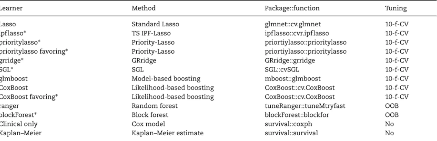
Following the terminology of the packagemlr [31], we denote a method configuration as a ‘learner’. There may be several learners based on the same method. An overview of learners considered in our benchmark study is displayed in Table1, while the full specification is given in the paragraph devoted to the corresponding method. In the following, the R packages used to implement the learners can be found in parentheses after the paragraph heading.
Penalized regression-based learners
Lasso (glmnet [39,40]). The penalty parameterλis chosen via
internal 10-fold CV. No group structure information is used.
SGL (SGL [41]). The model is fit via thecvSGLfunction. Tuning of
the penalty parameterλis conducted via internal 10-fold CV. The parameterαsteering the contribution of the group-Lasso and the standard Lasso is not tuned and set to the default value 0.95, as recommended by the authors [18]. All other parameters are set to default as well.
TS IPF-Lasso (ipflasso [42]). The penalty factors are selected in
the first step by computing separate ridge regression models for every feature group and averaging the coefficients within the groups by the arithmetic mean. These settings have shown reasonable results [16]. The choice of the penalty parametersλm
Table 1. Summary of learners used for the benchmark experiment.
Learner Method Package::function Tuning
Lasso Standard Lasso glmnet::cv.glmnet 10-f-CV
ipflasso∗ TS IPF-Lasso ipflasso::cvr.ipflasso 10-f-CV
prioritylasso∗ Priority-Lasso priortiylasso::prioritylasso 10-f-CV prioritylasso favoring∗ Priority-Lasso priortiylasso::prioritylasso 10-f-CV
grridge∗ GRridge GRridge::grridge 10-f-CV
SGL∗ SGL SGL::cvSGL 10-f-CV
glmboost Model-based boosting mboost::glmboost 10-f-CV
CoxBoost Likelihood-based boosting CoxBoost::cv.CoxBoost 10-f-CV CoxBoost favoring∗ Likelihood-based boosting CoxBoost::cv.CoxBoost 10-f-CV
ranger Random forest tuneRanger::tuneMtryfast OOB
blockForest∗ Block forest blockForest::blockfor OOB
Clinical only Cox model survival::coxph No
Kaplan–Meier Kaplan–Meier estimate survival::survival No
The use of group structure information is indicated with∗.
is conducted using 5-fold-CV in the first step and 10-fold CV in the second.
Priority-Lasso (prioritylasso [43]). The priority order is
deter-mined through a preliminary step realized in the same way as in the first step of TS IPF-Lasso. The priority-Lasso method takes into account the group structure. Even though the version with cross-validated offsets delivers slightly better prediction results [3], the offsets are not estimated via CV in order to not increase the computation times further. To select the parameter
λin each step of priority-Lasso, 10-fold CV is used.
Priority-Lasso favoring clinical features (prioritylasso [43]). The
set-tings are the same as before, except that the group of clinical variables is always assigned the highest priority. The preliminary step only determines the priority order for the molecular groups. The clinical variables are used as an offset when fitting the model of the second group. Furthermore, the clinical variables are not penalized (setting parameterblock1.penalization = FALSE).
GRridge (GRridge [44]). This method was not originally intended
for the purpose of including multi-omics group structure but is capable of doing so. To better fit the task at hand, a spe-cial routine was provided by the package author in personal communication. In addition, the argumentselectionENis set to TRUEso post-hoc variable selection is conducted, andmaxsel, the maximum number of variables to be selected, is set to 1000.
Boosting-based learners
Model-based boosting (mboost [45]). Internally,mlruses the
func-tionglmboostfrom the packagemboostand sets the family
argu-ment to CoxPH(). Furthermore, the number of boosting steps (mstop) is chosen by a 10-fold CV on a grid from 1 to 1000 viacvrisk. For the learning rateν the default value of 0.1 is used. Group structure information is not taken into account.
Likelihood-based boosting (CoxBoost [46]). The maximum number
of boosting stepsmaxstepnois set to default, i.e. 100. Again,mstopis determined by 10-fold CV. The penaltyλis set to default and thus computed according to the number of events. No group structure information is used.
Likelihood-based boosting favoring clinical features (CoxBoost [46]).
The settings are the same as before. Additionally, group structure information is used by specifying the clinical features as manda-tory. These features are favored as in the case of priority-Lasso by setting them as an offset and not penalizing them. Further
group information is not used, so the molecular data are not distinguished.
Random forest-based learners
Random forest (ranger [48]). Tuning of mtry is conducted via
thetuneMtryfastfunction of packagetuneRanger. The minimal
node size is 3 (the ranger default settings). The other hyper-parameters are set to default as well. Note that we also investi-gated therandomForestSRC[47] implementation of random forest, which leads to comparable results, but worked only on Windows and not on Ubuntu if parallelization was conducted via package
batchtools. We thus show only the results obtained withranger.
Block forest (blockForest [49]). Block forest is a random forest
variant able to include group structure information. The imple-mentation is based onranger. With functionblockforthe models are fit via the default settings.
Reference methods
The clinical reference model is a Cox proportional hazard model, computed via thecoxph function of thesurvival package [50] and only uses clinical features. The Kaplan–Meier estimate is computed viasurvfitfrom the same package.
Datasets
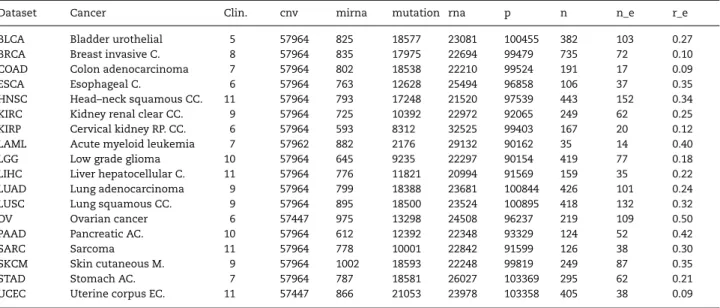
From the cancer datasets that have been gathered by the TCGA research network (http://cancergenome.nih.gov), we selected those with more than 100 samples and five different multi-omics groups, which resulted in a collection of datasets for 26 cancer types (a list of these 26 cancer types is provided in the supplement). As described below, further preprocessing eventually lead to 18 usable datasets. Table2gives an overview of these 18 datasets and the abbreviations used to reference them within the study.
For each cancer type, there are four molecular data types and the clinical data type, i.e. five groups of variables. The molecular data types comprise cnv, rna, miRNA expression (mirna) and mutation. It should be noted that the choice of data types was motivated by practical issues to a certain extent. In particular, methylation data would have been interesting to consider but could not be included due to their massive size, which would have led to long downloading and computation times. However,
Table 2.Summary of the datasets used for the benchmark experiment. The third to the seventh column show the number of features in the feature group, the eighth column the total amount of features (p). The last three columns show, in this order, the number of observations (n), the number of effective cases (n_e) and the ratio of the number of events and the number of observations (r_e).
Dataset Cancer Clin. cnv mirna mutation rna p n n_e r_e
BLCA Bladder urothelial 5 57964 825 18577 23081 100455 382 103 0.27 BRCA Breast invasive C. 8 57964 835 17975 22694 99479 735 72 0.10 COAD Colon adenocarcinoma 7 57964 802 18538 22210 99524 191 17 0.09
ESCA Esophageal C. 6 57964 763 12628 25494 96858 106 37 0.35
HNSC Head–neck squamous CC. 11 57964 793 17248 21520 97539 443 152 0.34 KIRC Kidney renal clear CC. 9 57964 725 10392 22972 92065 249 62 0.25 KIRP Cervical kidney RP. CC. 6 57964 593 8312 32525 99403 167 20 0.12 LAML Acute myeloid leukemia 7 57962 882 2176 29132 90162 35 14 0.40
LGG Low grade glioma 10 57964 645 9235 22297 90154 419 77 0.18
LIHC Liver hepatocellular C. 11 57964 776 11821 20994 91569 159 35 0.22 LUAD Lung adenocarcinoma 9 57964 799 18388 23681 100844 426 101 0.24 LUSC Lung squamous CC. 9 57964 895 18500 23524 100895 418 132 0.32
OV Ovarian cancer 6 57447 975 13298 24508 96237 219 109 0.50
PAAD Pancreatic AC. 10 57964 612 12392 22348 93329 124 52 0.42
SARC Sarcoma 11 57964 778 10001 22842 91599 126 38 0.30
SKCM Skin cutaneous M. 9 57964 1002 18593 22248 99819 249 87 0.35
STAD Stomach AC. 7 57964 787 18581 26027 103369 295 62 0.21
UCEC Uterine corpus EC. 11 57447 866 21053 23978 103358 405 38 0.09 Abbreviations: C. indicates carcinoma; CC., cell carcinoma; PP, renal papilla; AC., adenocarcinoma; M., melanoma; EC., endometrial carcinoma.
such compromises for practical reasons are inevitable and other data types could have been considered.
The number of variables differs strongly between groups but is similar across datasets. Most molecular features (about 60 000) belong to the cnv group but only a few hundred features to mirna, the smallest group. There is a total of about 80 000 to 103 000 molecular features for each cancer type.
Of the 26 available datasets, three were excluded because they did not have observations for every data type. Furthermore, since the outcome of interest is survival time, not only the number of observations is crucial but, most importantly, the number of events (deaths), which we call the number of effective cases. A ratio of 0.2 of effective cases is common [10]. The five datasets that had less than 5% effective cases were excluded.
Since the majority of the clinical variables had missing val-ues, the question arose of which to include for a specific dataset while saving as many observations as possible. As we did not have any domain knowledge, we adopted a two-step strategy. Firstly, an informal literature search was conducted to find stud-ies where the specific cancer type was under investigation. Variables mentioned to be useful in these studies were included, if available. Secondly, we additionally used variables that were available for most of the cancer types. These comprised sex, age, histological type and tumor stage. These were included as standard, if available. Of course, sex was not included for the sex-specific cancer types.
Finally, note that our study considers only one dataset per cancer type, i.e. per prediction problem. It evaluates the can-didate learners using CV, which reasonably estimates the pre-diction performance that would be obtained for a population with similar characteristics (in statistical terms, with similarly distributed data). From a practical clinical perspective, it is cru-cial to evaluate prediction rules on independent external data before implementing them in practice. The resulting estimated prediction performance is usually less impressive than the CV estimate [51]. However, although some discrepancies between the rankings can be observed, the difference between rankings is less prominent than the difference between errors. We assume
that methods performing best in CV also range among the best ones when applied to external datasets, which is compatible with the extensive results presented in Bernauet al.[52].
Results
Failures and refinement of the study design
As a consequence of the repeated 5-fold CV, 11·10·5+7·5· 5=725 models are fit for each learner in total. Some of these model fittings—i.e. some CV iterations—were not successful. This is common in benchmark experiments of larger scale [53]. Such a failure does not affect the other 4 CV iterations and the remaining nine repetitions of CV but leads to missing values for the assessment measures for the failing iterations, which have to be handled when computing averaged measures. To cope with such modeling failures, we follow strategies described previously [53,54]. If a learner fails in more than 20% of the CV iterations for a given dataset, we assign (for the failing iterations) values of the performance measures corresponding to random prediction (0.25 for ibrier and 0.5 for cindex) and the mean of the other iterations for the computation time and the number of selected features. If a learner fails in less than 20%, the performance means of the successful iterations are assigned for all measures. See Table4 for the learners’ failure rates averaged over the datasets.
Modeling failures are mainly learner related, that is, there are no datasets for which many or all learners are unstable, but individual learners are particularly unstable. For every dataset, there are at least seven learners yielding no failures. In contrast, learners Lasso, CoxBoost and glmboost are rather unstable, with 31.2%, 28.6% and 19.7% failures in total. IPF-Lasso is more stable overall, but also considerably unstable for specific datasets. The other learners are very stable, with not a single failure for the random forest variants, the reference methods and CoxBoost favoring. Dataset specific failure rates can be taken from the tables in the supplement, which show the learner performances like in Table4broken down by dataset.
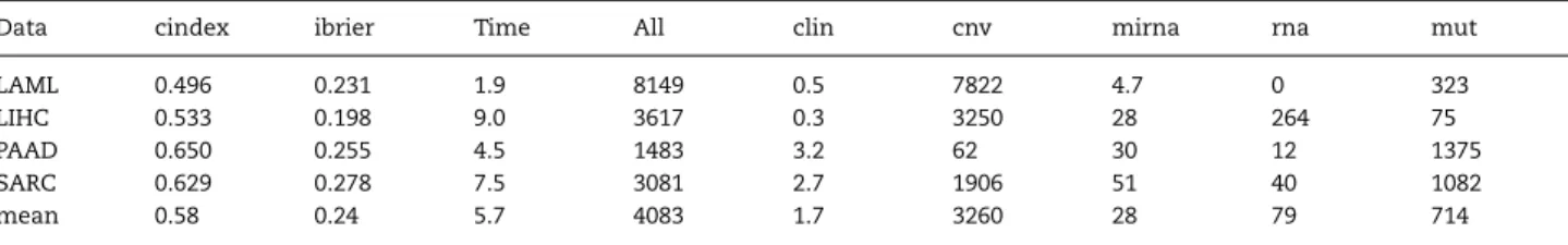
Table 3.Performance of SGL on four small datasets. Column ‘All’ represents the total number of selected features, the subsequent columns the numbers of selected features of the respective groups.
Data cindex ibrier Time All clin cnv mirna rna mut
LAML 0.496 0.231 1.9 8149 0.5 7822 4.7 0 323
LIHC 0.533 0.198 9.0 3617 0.3 3250 28 264 75
PAAD 0.650 0.255 4.5 1483 3.2 62 30 12 1375
SARC 0.629 0.278 7.5 3081 2.7 1906 51 40 1082
mean 0.58 0.24 5.7 4083 1.7 3260 28 79 714
Besides such modeling failures, more general issues related to usability occurred while conducting the experiment. First of all, using SGL with the considered large numbers of fea-tures always leads to a fatal error in R under Windows, but not using the Linux distribution Ubuntu 14.04. More importantly, the extremely long computation times for SGL were problematic. Since we received no feedback from the authors, we used the standard settings. These lead to computations lasting several days for one single model fit for large datasets. Altering some of the parameters did not strongly reduce the computational burden. Running the whole experiment as planned was thus not possible for SGL. Here, we briefly present the results of SGL which could be obtained based on four of the smallest datasets. For the rest of the study we exclude SGL from the analysis. On average, over all iterations and the four datasets, SGL leads to a cindex of 0.58 and an ibrier of 0.24. The resulting models are neither sparse on feature level, with an average of 4083 selected features, nor on group level. The mean computation time of 5.7 h for one CV iteration confirms the problem of extremely long computation times. In comparison, the next slowest method needs 1.2 h for one iteration, on average over all datasets. Table3 shows the performance values of SGL for each of the four datasets and the mean values.
Computation time
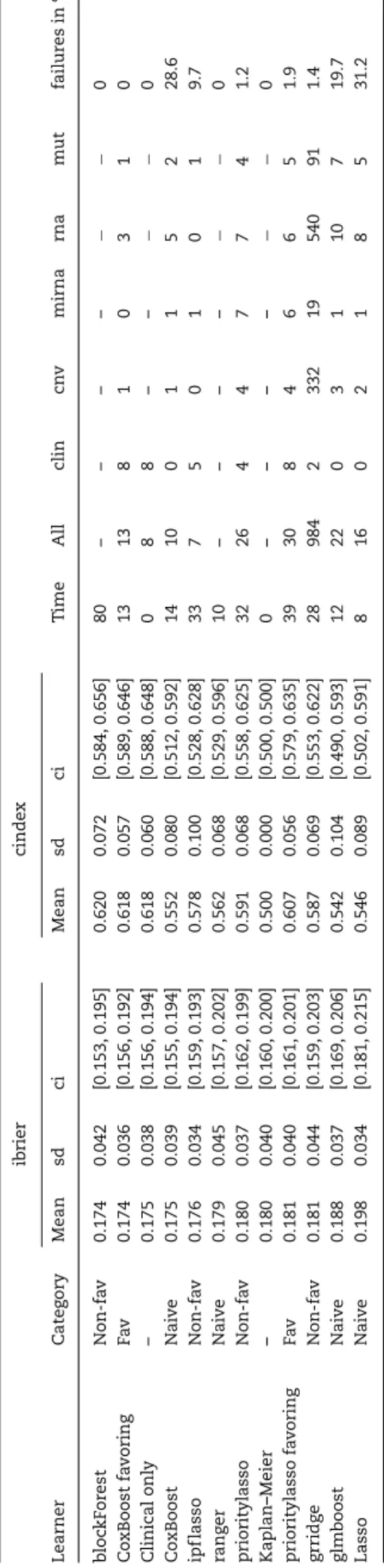
Table4 shows the average performance measures for every method and is ordered by the ibrier. All values are obtained by— firstly—averaging over the outer-resampling CV iterations and— secondly—averaging over the datasets. For the methods not yielding model coefficients the corresponding cells contains ‘-’. The ninth column of Table4displays the mean computation time. The computation times are measured as the time needed for model fitting (training time). The fastest procedures are stan-dard Lasso and ranger, followed by glmboost and the CoxBoost variants. The three penalized regression methods using group structure (IPF-Lasso, priority-Lasso, GRridge) are about two to three times slower, with GRridge being the fastest of the three methods. Of the two prioritylasso variants the one favoring clin-ical features is a little slower. Finally, blockForest is the slowest method.
Of course, the computation times depend on the size of the datasets. Figure1displays the mean computation time of one outer-resampling iteration for the different learners and datasets. The datasets are ordered from smallest (LAML) to largest (BRCA).
The long computation times of priority-Lasso and IPF-Lasso for COAD and KIRP are notable. COAD and KIRP are among the smaller datasets with 17 (9%) and 20 (12%) events, respectively. Generally, computation times vary more over the CV iterations for these methods. For KIRP and COAD this variation is partic-ularly strong, with individual model fittings taking up to 50 h.
However, the CV iterations which lead to these extreme compu-tation times for IPF-Lasso and priority-Lasso, lead to modeling failures for the unstable learners Lasso, glmboost and CoxBoost. That means, especially priority-Lasso and to lesser extent IPF-Lasso are more stable for particular CV iterations than the unstable learners, but this comes at the price of increased computation times. Note, moreover, all Lasso variants rely on the same implementation of Lasso (glmnet). The more specific methods improve the Lasso approach in terms of stability, because where standard Lasso fails, often the more specific variants do not.
Model sparsity
To assess sparsity, the number of nonzero coefficients of the resulting model of each CV iteration is considered. As random forest models do not yield such coefficients, this aspect is not assessed for random forest variants.
Sparsity on the level of variables
Sparsity in terms of the number of included variables is par-ticularly interesting for practical purposes, since sparse models are easier to interpret and to communicate. On average, as Table4shows, ipflasso leads to the sparsest models with an average of seven variables, followed by CoxBoost with on average 10 variables. CoxBoost favoring and Lasso are also reasonably sparse (13, 16), but the variability is higher for Lasso (Figure2). glmboost, prioritylasso and prioritylasso favoring yield models with more than 20 features (22, 26, 30). Least sparse is grridge; the average grridge model size (984) is close to the maximum number of features to be selected (maxsel = 1000). grridge seems not to be able to appropriately select variables in this setting (recall that it is not intended to do so).
Sparsity on group level
Table4(see also Figure 1 in the supplement) shows that grridge and priority-Lasso choose variables from all groups and are thus not sparse on group level. Among the other methods, IPF-Lasso yields strong sparsity on group level. Mostly clinical fea-tures are selected. Furthermore, with boosting variants CoxBoost and glmboost and with standard Lasso no clinical features are selected. CoxBoost favoring does not select mirna features. IPF-Lasso does not include cnv and rna features. This exemplifies the problem of methods treating high- and low-dimensional groups equally. As already pointed out, due to their low dimension, clinical variables get lost within the huge number of molecular variables. It becomes obvious that this also applies for some of the molecular variables. The mirna group is, in comparison with the other molecular groups, lower dimensional with 585 to 1002 features. Learners which do not consider group structure fail to include clinical variables and include at most one mirna
Ta b le 4 . A v er a g e learner performances. T he v a lues ar e o btained b y a v er a g ing o v e r the CV iter ations and d atasets. The time is measur e d in m in utes. T he second co lumn sho w s the aff iliation of the methods using the m u lti-omics d ata to the cate gories described in section 3.3. Column ‘A ll’ re pr esents the total n umber o f selected featur e s, the subsequent columns the n umbers of selected featur es of the respecti v e g ro ups. F o r learners n ot yielding model coeff icients, the corr e sponding measur e s a re set to “-”. T he ‘ci’ columns displa y the 95% conf idence interv a ls for the means based on quantiles o f the t-distribution; observ ations ar e the learners’ a v er a g e v alues o v e r the CV iter ations, i.e . o ne observ ation p er dataset. The tota l n u m b e r o f fe a tu re s m a y d if fe r fro m th e su m o f featur es in eac h gr oup d ue to ro unding err o rs. T he last column de picts the o v er all p er centa g e o f m odeling failur e s. ibrier cinde x Learner C ate g or y M ean sd ci Mean sd ci T ime All clin cn v m irna rna m ut failur e s in % b loc kF or est N on-fa v 0.174 0.042 [0.153, 0.195] 0.620 0.072 [0.584, 0.656] 80 – – – – −− 0 Co xBoost fa v oring Fa v 0.174 0.036 [0.156, 0.192] 0.618 0.057 [0.589, 0.646] 13 13 8 1 0 3 1 0 Clinical onl y – 0 .175 0.038 [0.156, 0.194] 0.618 0.060 [0.588, 0.648] 0 8 8 – – −− 0 Co xBoost N ai v e 0.175 0.039 [0.155, 0.194] 0.552 0.080 [0.512, 0.592] 14 10 0 1 1 5 2 2 8.6 ipf lasso Non-fa v 0 .176 0.034 [0.159, 0.193] 0.578 0.100 [0.528, 0.628] 33 7 5 0 1 0 1 9 .7 ra ng er Nai v e 0 .179 0.045 [0.157, 0.202] 0.562 0.068 [0.529, 0.596] 10 – – – – −− 0 prioritylasso Non-fa v 0 .180 0.037 [0.162, 0.199] 0.591 0.068 [0.558, 0.625] 32 26 4 4 7 7 4 1 .2 Kaplan–Meier – 0 .180 0.040 [0.160, 0.200] 0.500 0.000 [0.500, 0.500] 0 – – – – −− 0 prioritylasso fa v o ring Fa v 0 .181 0.040 [0.161, 0.201] 0.607 0.056 [0.579, 0.635] 39 30 8 4 6 6 5 1 .9 grridg e N on-fa v 0.181 0.044 [0.159, 0.203] 0.587 0.069 [0.553, 0.622] 28 984 2 332 19 540 91 1.4 glmboost N ai v e 0.188 0.037 [0.169, 0.206] 0.542 0.104 [0.490, 0.593] 12 22 0 3 1 1 0 7 19.7 Lasso Nai v e 0 .198 0.034 [0.181, 0.215] 0.546 0.089 [0.502, 0.591] 8 1 6 0 2 1 8 5 31.2
variable. CoxBoost favoring, which differentiates clinical and molecular variables, does not select mirna features. In contrast, learners taking into account the multi-omics group structure generally include variables of both lower dimensional groups. Using the group structure thus prevents low-dimensional groups from being discounted.
Prediction performance
Overview and main findings
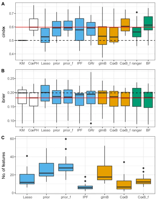
Figure2shows the distributions of the values of the performance metrics across the datasets. Again, grridge is excluded from the sparsity panel. Three important findings can be highlighted. First of all, regarding Figure2, most of the learners perform better than the Kaplan–Meier estimate (indicated by the dashed horizontal line). This indicates that using the variables is, in general, useful. Only Lasso performs worse than the Kaplan– Meier estimate (based on the ibrier). Secondly, only blockForest outperforms the reference clinical Cox model (red horizontal line), which stresses the importance of the clinical variables for these datasets. Finally, methods taking into account the group structure in some way in general outperform the naive methods.
Comparing prediction methods
All analyses in this section refer toTable 4.
Naive methodsThe learners CoxBoost, glmboost, ranger and standard Lasso are fit with the naive strategy. In general, the results are not consistent over the two measures. With regards to the ibrier, likelihood-based boosting performs best. Moreover, model-based boosting performs better than Lasso but gets out-performed by random forest which is close to likelihood-based boosting. According to the cindex, random forest performs best followed by likelihood-based boosting and Lasso. Model-based boosting performs the worst. All methods are at least slightly better than the Kaplan–Meier estimate. To sum up, although the results differ depending on the considered measure, random forest shows a tendency to outperform the other methods, since it is among the best methods based on the ibrier and performs best based on the cindex.
Methods not favoring clinical featuresThe learners block forest, ipflasso, prioritylasso and grridge use the group structure but do not favor clinical features. The random forest variant blockForest outperforms the other methods. It performs better on average than any other method based on both measures. Among the penalized regression methods, IPF-Lasso performs best according to the ibrier and priority-Lasso according to the cindex. GRridge ranks third according to the ibrier and second according to the cindex. Moreover, priority-Lasso and GRridge perform equal to or even worse than the Kaplan–Meier estimate based on the ibrier. Since IPF-Lasso yields the sparsest models, it might be preferable when sparsity is important.
Methods favoring clinical featuresThere are two learners favoring clinical features: CoxBoost favoring and prioritylasso favoring. The results are unambiguous with CoxBoost favoring performing better than prioritylasso favoring. Furthermore, both learners perform better than the Kaplan–Meier estimate based on the cindex, but only CoxBoost favoring performs better than the Kaplan–Meier estimate based on the ibrier. Thus, according to these findings, likelihood-based boosting yields better results than priority-Lasso when clinical variables are favored, even though priority-Lasso here further distinguishes the molecular data.
Figure 1. Computation time. (A) Computation times in seconds. (B) Computation times in log(seconds). The datasets are ordered form smallest (LAML) to largest (BRCA).
However, when comparing the described performances— especially if based on the aggregated results in Table 4—it is very important to consider the heterogeneity over the datasets. As the standard deviations and confidence intervals inTable 4 and the boxplots in Figure 2 show, the performance of the methods varies strongly over the datasets (the confidence intervals are obtained by using the learners’ average values over the CV iterations as observations, i.e. one observation per dataset). The dataset specific learner performances are depicted in the supplementary tables. Moreover, paired two-sidedt-tests comparing, for example, blockForest with CoxBoost favoring and the clinical only model show no statistically significant differences in performance with p-values of 0.81 and 0.86 (cindex) and 0.95 and 0.78 (ibrier). For allt-tests in the study, the normal distribution assumption was checked with Shapiro–Wilk tests and Q-Q plots. Thus, considering the small differences in performance and the variability of the method performances across datasets, conclusions about the superiority of one method over another should be treated with great caution.
Using multi-omics data
In the first part of this section, we summarize our results regard-ing the added predictive value of multi-omics as a by-product of our benchmark study, before eventually focusing on the method-ological comparison of the different approaches of taking the structure of the clinical and multi-omics variables into account. Added predictive valueTo assess the added predictive value of the molecular data, we follow approach A proposed by Boulesteix and Sauerbrei [2], thus comparing learners obtained by only using clinical features and combined learners, i.e. learners using clinical and molecular variables. Since it is emphasized that for this validation approach the combined learners should not be derived by the naive strategy, these learners are not considered here.
In general, the findings indicate that the multi-omics data may have the potential to add predictive value. First of all, blockForest outperforms the Cox model based on both measures. Secondly, as Table5shows, there are several datasets for which there is at least one learner that takes the group structure into account and outperforms the clinical learner. For some of the
Figure 2. Performance of the learners. A: cindex. B: ibrier. C: total number of selected features; only learners yielding model coefficients are included and grridge is excluded since it yields models on a much larger scale. The solid red and dashed black horizontal lines correspond to the median performance of the clinical only model and the Kaplan–Meier estimate, respectively. Colors indicate membership to one of the general modeling approaches: penalized regression (blue), boosting (orange), random forest (green), reference methods (white). Abbreviations: KM indicates Kaplan–Meier; Lasso, Lasso; glmB, glmboost; CoxB, CoxBoost; CoxPH, clinical only; prior, priority-Lasso; prior_f, priority-Lasso favoring; IPF, ipflasso; CoxB_f, CoxB favoring; GRr, grridge; BF, blockForest; ranger, ranger.
datasets, e.g. LAML and COAD, the performance differences are substantial. Thus, using additional molecular data leads to better prediction performances in some of the considered cases. On the other hand, it must be taken into account that in the other cases the differences are small and, again regarding the confidence intervals, one has to be careful when drawing conclusions about the superiority over the Cox model. Moreover, for six datasets the Cox model does not get outperformed by methods which use the omics data. This raises serious concerns regarding a beneficial effect of the omics data as far as the considered TCGA data are concerned.
Including group structure In general, the results suggest that using the naive strategy of treating clinical and molecular
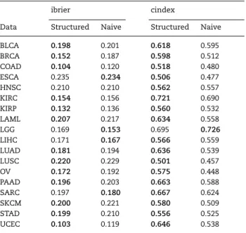
variables equally leads to a worse performance in comparison to methods that take the group structure into account. Table6 shows the mean performance of the naive learners and the structured learners (both favoring and not favoring the clinical features) by dataset. That is, we compare methods using multi-omics data and additionally its structure (structured learners: ipflasso, priortylasso variants, grridge, CoxBoost favoring, blockForest) against methods using the multi-omics data but not taking into account its structure (naive learners: Lasso, ranger, CoxBoost, glmboost). The clinical only model and the Kaplan–Meier estimate are not considered here. Each value is computed as average over the naive respectively the structured learners’ mean cindex and ibrier values. Only in five cases is
Ta b le 5 . Assessment of the a dded p re dicti v e v alue of the m olecular v a ria b les b y d ataset. T he second and se v enth column sho w the best performing learners for th e respecti v e d ataset and measur e , the ‘cinde x ’ a nd ‘ibrier’ columns the p erformances o f these learners. In the cases wher e the clinical onl y model is o utperformed, the ‘Ref. ’ columns sho w the corr esponding cinde x a nd ibrier v a lues of the refer ence C o x model o nl y u sing clinical v a ria b les. The “ci” columns sho w the 95% conf idence interv a ls for the re specti v e performance v a lues based o n q uantiles o f the t-distribution; observ ations ar e the learners’ CV iter ation v alues. Note that these interv a ls ar e intended to g iv e a n otion o f the sta bility o f the mean v alues, but a re —in contr ast to T a b le 4 —not v alid conf idence interv als, since the CV iter ations ar e n o inde p endent observ ations [ 55 , 56 ]. Bold letters indicate datasets for w hic h ther e is a method u sing the g ro up structur e and o utperforming the C o x model for b oth measur e s. Data Learner ibrier ci R ef. ci Learner cinde x ci R ef. ci BLC A Co xBoost fa v oring 0 .190 [0.181, 0.199] 0.192 [0.183, 0.201] Co xBoost fa v oring 0 .640 [0.612, 0.668] 0.633 [0.607, 0.659] BRC A b loc kF or est 0 .141 [0.134, 0.149] 0.147 [0.137, 0.158] Co xBoost fa v oring 0 .643 [0.618, 0.669] 0.637 [0.608, 0.666] CO AD b loc kF or est 0 .087 [0.075, 0.099] 0.101 [0.088, 0.115] b loc kF or est 0 .656 [0.586, 0.725] 0.541 [0.475, 0.608] ESC A ipf lasso 0.209 [0.198, 0.221] 0.214 [0.199, 0.228] Clinical onl y 0.574 [0.536, 0.612] −− HNSC glmboost 0 .202 [0.193, 0.211] 0.210 [0.201, 0.220] b loc kF or est 0 .582 [0.554, 0.610] 0.554 [0.519, 0.588] KIRC ipf lasso 0.144 [0.138, 0.149] 0.146 [0.140, 0.152] Clinical onl y 0.761 [0.734, 0.789] −− KIRP ra ng er 0.118 [0.106, 0.131] 0.140 [0.117, 0.163] grridg e 0 .629 [0.566, 0.692] 0.572 [0.502, 0.641] LAML ra ng er 0.182 [0.165, 0.199] 0.231 [0.200, 0.263] ra ng er 0.709 [0.651, 0.766] 0.596 [0.534, 0 .657] LGG Lasso ∗ 0.145 [0.132, 0.157] 0.168 [0.154, 0.181] glmboost 0 .749 [0.719, 0 .779] 0.652 [0.618, 0.685] LIHC ra ng er 0.146 [0.135, 0.157] 0.169 [0.158, 0.180] grridg e 0 .602 [0.560, 0.645] 0.586 [0.542, 0 .630] LU AD Co xBoost fa v oring ∗ 0.172 [0.160, 0.183] 0.172 [0.161, 0.183] prioritylasso 0.665 [0.640, 0.690] 0.663 [0.631, 0.695] LUSC grridg e 0 .210 [0.203, 0.217] 0.216 [0.205, 0.227] prioritylasso fa v o ring 0.537 [0.502, 0 .572] 0.531 [0.502, 0 .561] OV ipf lasso ∗ 0.169 [0.163, 0.174] 0.173 [0.167, 0.179] prioritylasso 0.600 [0.582, 0.618] 0.598 [0.580, 0.617] PAAD Clinical onl y ∗ 0.190 [0.178, 0.202] – – prioritylasso fa v o ring 0.686 [0.658, 0.714] 0.683 [0.655, 0.712] SARC glmboost ∗ 0.179 [0.167, 0.190] 0.202 [0.188, 0.217] b loc kF or est 0 .685 [0.651, 0.720] 0.673 [0.637, 0.709] SKCM Clinical onl y 0.191 [0.185, 0.198] 0.191 [0.185, 0.198] b loc kF or est 0 .597 [0.556, 0.639] 0.581 [0.540, 0.623] ST AD Clinical onl y 0.192 [0.182, 0.202] – – Clinical onl y 0.598 [0.555, 0.641] – – UCEC ipf lasso 0.091 [0.079, 0.102] 0.092 [0.080, 0.105] Clinical onl y 0.686 [0.581, 0.791] – – ∗indicates that ther e is a m ethod w ith e qual performance .
Table 6. Comparing naive learners and structured learners. The performance of structured learners, i.e. learners using the group structure, and naive learners are compared for every dataset. The cindex and ibrier columns show the mean performance values for the corresponding dataset and learner types. Bold values indicate better values for the given dataset.
ibrier cindex
Data Structured Naive Structured Naive
BLCA 0.198 0.201 0.618 0.595 BRCA 0.152 0.187 0.598 0.512 COAD 0.104 0.120 0.518 0.480 ESCA 0.235 0.234 0.506 0.477 HNSC 0.210 0.210 0.562 0.557 KIRC 0.154 0.156 0.721 0.690 KIRP 0.132 0.136 0.560 0.532 LAML 0.207 0.217 0.634 0.558 LGG 0.169 0.153 0.695 0.726 LIHC 0.171 0.167 0.566 0.559 LUAD 0.181 0.194 0.636 0.539 LUSC 0.220 0.229 0.501 0.457 OV 0.172 0.192 0.575 0.448 PAAD 0.196 0.203 0.663 0.588 SARC 0.197 0.180 0.667 0.624 SKCM 0.200 0.221 0.580 0.509 STAD 0.199 0.210 0.556 0.525 UCEC 0.103 0.119 0.646 0.538
the average performance of the naive learners better than the average performance of the structured learners: regarding the ibrier, the naive learners perform better than the structured learners for four datasets; regarding the cindex, only for the LGG dataset is the performance of the naive learners higher than the performance of the structured learners. Unpaired, one-sided t-tests for the four naive and the six structured learners, using the mean performance values of the individual methods over the datasets as observations, yieldp-values of 0.1273 and 0.0002 for the ibrier and cindex, respectively.
In summary, if multi-omics data are used—although there is a general concern regarding the usefulness of models using multi-omics compared with simple clinical models—its struc-ture should also be taken into account.
Favoring clinical featuresAccording to our findings, favor-ing clinical variables leads to better prediction results. For likelihood-based boosting, this is in line with the findings of others (see [57] and the reference therein). Differentiating the clinical variables from the molecular features strongly increases the prediction performance of likelihood-based boosting (CoxBoost and CoxBoost favoring), according to the average cindex. Favoring clinical features raises likelihood-based boosting from one of the worst to one of the best performing methods. Moreover, our findings show this might also hold for methods which use the multi-omics group structure. For priority-Lasso the increase is not as strong, but still notable when considering the cindex. Yet, the ibrier does not confirm this.
Discussion
In general, one should be very careful when interpreting the results of our benchmark experiment and drawing conclusions. Most importantly, the findings highly depend on the consid-ered prediction performance measure, as the method ranking
changes drastically between the two measures. For example, CoxBoost performs poorly based on the cindex but performs third best regarding the ibrier. These findings indicate that the performance of a method may change dramatically if a differ-ent performance measure is used for its assessmdiffer-ent. Moreover, according to ibrier, two methods perform better than the Cox model (though only slightly), and six methods perform worse than the Kaplan–Meier estimate. Generally, since the cindex only measures discrimination and is not a strictly proper scoring rule, the ibrier should be considered more important. In particular, if prognostic accuracy is of interest, preference should be given to the ibrier. However, given its interpretability, the cindex could be preferred if risk classification is the main objective.
Another important aspect of the performance assessment is, as shown in Figure2and Table5, the variability across datasets. The superiority of one method over the other strongly depends not only on the considered performance measure but also, most importantly, on the considered datasets. This stresses the impor-tance of large-scale benchmarks, like this one, which use many datasets. Since the variability between datasets is huge, we need many datasets—a fact well known by statisticians performing sample size calculations, which however tends to be ignored when designing benchmark experiments using real datasets [58]. If we had conducted our study with, say, 3, 5 or 10 datasets (as usual in the literature), we would have obtained different— more unstable—results.
Regarding prediction performance, blockForest outperforms the other methods on average overall datasets. Moreover, it is the only method which outperforms the simple Cox model on average regarding both measures. The other methods using the molecular data do not perform better than the simple Cox model. The better prediction performance of blockForest, how-ever, comes at the price of long computation times. Apart from SGL, blockForest is the slowest method. The fastest learners, standard Lasso and ranger, are about 10 times faster and block-Forest is still 2 times slower than the next slowest learner prioritylasso favoring. Moreover, like the standard random for-est variant, it does not yield easily interpretable models, even though the strengths of the variables can be assessed via the variable importance measure(s) output as a by-product of the random forest algorithms. Thus, taking the other assessment dimensions into account, e.g. CoxBoost favoring clinical features is very competitive. It is quite fast, leads to reasonably sparse models at group and feature level and yields performances only slightly worse than (cindex) or equal to (ibrier) blockForest.
From a practical perspective, even simpler modeling approaches, such as a simple Cox model using clinical variables only, might be preferable. This model is easily interpretable, needs only a fraction of the computation time and, with a mean cindex of 0.618 and a mean ibrier of 0.175, performs only slightly worse than blockForest (0.620 and 0.172) and comparable to or even better than all other methods. Note, however, that blockForest also offers the possibility of favoring clinical covariates using the argumentalways.select.blockof the
blockforfunction. Hornung and Wright [27] show that this can
improve the prediction performance of block forest considerably. However, since this option was not yet available at the time of conduction of the analyses performed for the current paper, we were not able to consider this block forest variant here.
In general, conclusions about the superiority of one method over the other with respect to the prediction performance must be drawn with caution, as the differences in performance can be very small and the confidence intervals often show a remarkable overlap. Exemplaryt-tests comparing blockForest with CoxBoost
favoring and the Clinical only model showed no significant differences in performance. Furthermore, we do not believe that the recommendation of a single method is generally appropriate because even if some methods have a better average perfor-mance than others, the ranking between methods depends in large part on the specific dataset used. On the other hand, if there is no independent, external dataset available for performance estimation it is also not advisable to try out too many methods in practice because this increases the risk that the maximum of the cross-validated performance estimates is optimistic [59] and correction methods to adjust for this over-optimism are still in their infancy [60]. In this situation, it is likely best to strike a balance by taking into account the learners which perform reasonably well. Our study identifies methods worth taking into closer consideration in practice. Apart from the clinical model, these are all methods which take the multi-omics structure into account or favor the clinical covariates, as on average those methods performed better than the naive methods not using the group structure (note again, however, that we did not observe statistically significant differences). A method should then be chosen based on the methodology described in the paper using the dataset at hand.
More generally, it should be noted that the choice of a method should result from the simultaneous consideration of various aspects beyond performance. If (i) performance is the main criterion, (ii) the model is intended solely as a prediction tool, and implemented, say, as a shiny application [61], and (iii) sparsity and interpretability are not considered important, blockForest is certainly a very good choice. Other methods may prove attrac-tive in different situations. Finally, let us note that one of the methods that did not perform very well in the present study in terms of performance, priority-Lasso, may perform better in practice when accurate prior knowledge on the groups of variables is available, and allows the user to favor some of the groups—a dimension that could not be taken into account in our comparison study.
A potential limitation of our study is that the datasets were already used by Hornung and Wright [27] in their comparison study. Since they selected the most promising blockForest based on this comparison study, our results may be slightly optimistic regarding the performance of blockForest—a bias mechanism that has been previously described [62]. More precisely, Hor-nung and Wright [27] initially considered five different variants of random forest taking the block structure into account and identified the best-performing variant using a collection of 20 datasets including the 18 considered in our study. They named this best-performing variant ‘block forest’. It is in theory possible that part of the superiority of the selected ‘block forest’ variant on the specific 20 datasets is due to chance. In this case, our study, which uses 18 of these datasets again, would (slightly) favor block forest. However, this over-optimism only exists if a different one of the five Block Forest variants compared in the Block Forest paper were the best in reality, i.e. if the superiority of the Block Forest variant considered in our paper were just the result of random fluctuations in the paper of Hornung and Wright [27]. Given the fact that Hornung and Wright [27] used a lot of datasets this is rather unlikely and it is plausible that block forest is indeed the best option, in which case the over-optimistic effect for our study can be ruled out. In addition, although our study is based on data from the same cancer stud-ies, there are several notable differences. Hornung and Wright [27] included two additional datasets and did not use the same sets of clinical variables as in our study. Furthermore, to reduce the computational burden, they used only a subset of 2500
variables when groups had more than 2500 variables. Taking all these aspects into account, it is unlikely that our study is noticeably biased, although such a bias is possible in principle. Regarding the advantage of favoring the clinical variables, it is important to note that it strongly depends on the level of predictive information contained in these variables. If clinical variables contain less information than for the datasets used in our analysis, favoring of these covariates might be less useful than they were found to be in this study, or even detrimental. While we strongly recommend considering favoring the clinical variables, this should not necessarily be performed by default.
Another limitation of our study is that it is based on CV—as usual in the context of large-scale benchmarking. We assume that methods performing best in CV also range among the best ones when applied to external datasets, which is compat-ible with the results presented in Bernauet al.[52]. However, in principle, differences may occur. For example, the perfor-mance of methods tending to strongly overfit the training data is expected to drop more when considering external data instead of using CV than the performance of methods that do not strongly overfit. These subtle issues could be addressed in future studies using the recently suggested cross-study validation tech-nique. This approach, however, requires the availability of sev-eral external datasets for each cancer type that include exactly the same prediction and outcome variables and consider com-parable target populations. Currently, such data is simply not available.
Extending the benchmark to further methods (e.g. methods that do not rely on the proportional hazards assumption, which are only represented by random forest in our study) and further data pre-processing approaches as well as further datasets are desirable. In the same vein, it may be interesting to consider alternative procedures to handle model failures in the outer-resampling process, which may lead to different results. There is to date no widely used standardized approach to deal with missing values in this context. This issue certainly deserves fur-ther dedicated research. This benchmark experiment is designed such that such extensions are easy to implement. Using the provided code, further methods can be compared to the ones included in this study.
Key Points
•For the collection of the datasets used in this study, the standard Cox model only using clinical variables is very competitive compared with complex methods using multi-omics data. Among the investigated com-plex methods, only block forest outperforms the Cox model on average over all datasets, and the difference is not statistically significant.
•If multi-omics data is used, its structure should be used as well: on average it increases the predictive performance and prevents low-dimensional feature groups from being discounted.
•Favoring clinical variables over molecular data in-creases the prediction performance of the investigated methods on average.
•In general, the findings indicate that assessing and comparing prediction methods should be based on a large number of datasets to reach robust conclusions. •Aside from the main results of the study, we also observed that using multi-omics data can improve