Smart information retrieval: domain knowledge centric optimization approach

(1)

Smart Information Retrieval: Domain Knowledge

Centric Optimization Approach

Abduladem Aljamel, Taha Osman, Member, IEEE, Giovanni Acampora, Senior Member, IEEE, Autilia Vitiello,

Member, IEEE, Ziqi Zhang Abstract— In the age of Internet of Things (IoT), online data

has witnessed significant growth in terms of volume and diversity, and research into information retrieval has become one of the important research themes in the Internet oriented data science research. In information retrieval, machine-learning techniques have been widely adopted to automate the challenging process of relation extraction from text data, which is critical to the accuracy and efficiency of information retrieval-based applications including recommender systems and sentiment analysis. In this context, this paper introduces a novel, domain knowledge centric methodology aimed at improving the accuracy of using machine-learning methods for relation classification, and then utilise Genetic Algorithms (GAs) to optimise the feature selection for the learning algorithms. The proposed methodology makes significant contribution to the processes of domain knowledge-based relation extraction including interrogating Linked Open Datasets to generate the relation classification training-data, addressing the imbalanced classification in the training datasets, determining the probability threshold of the best learning algorithm, and establishing the optimum parameters for the genetic algorithm utilised in feature selection. The experimental evaluation of the proposed methodology reveals that the adopted machine-learning algorithms exhibit higher precision and recall in relation extraction in the reduced feature space optimised by the implementation. The considered machine learning includes Support Vector Machine, Perceptron Algorithm Uneven Margin and K-Nearest Neighbours. The outcome is verified by comparing against the Random Mutation Hill-Climbing optimisation algorithm using Wilcoxon signed-rank statistical analysis.

Index Terms—IoT, Information Extraction, Smart System,

Machine Learning, Genetic Algorithms, Optimization

I.INTRODUCTION

NTERNET of Things (IoT) paradigm is increasing the amount of data being made available online [1][2]. It is due to the integration of the Internet with many heterogeneous areas such as, Internet of Healthcare Things (IoHT) in medical, Internet of Vehicles (IoV) in transport, and Internet of Industrial Things (IIoT) in industry [3][4]. The growing online data can be analysed to satisfy the information need of a variety of intelligent or smart applications and services including advising financial investors about a potential business risk, informing the music industry about an emerging consumer trend, alerting drivers using traffic predictions, etc. [5]. However, the online-published data is diverse in terms of volume and complexity, largely unstructured and constructed in natural human languages, which makes its manual exploitation infeasible.

A. Aljamel and T. Osman are with Dept. of Computing, Nottingham Trent University, NG11 8NS, UK (email: [email protected] and [email protected])

G. Acampora is with Department of Physics, University of Naples Federico II, 80126 Naples, Italy (email: [email protected])

A. Vitiello is with Department of Computer Science, University of Salerno, Fisciano 84084, Italy (email: [email protected]).

Z. Zhang is with the Information School, University of Sheffield, UK (email: [email protected]).

Therefore, Information Extraction (IE) techniques are needed to automate the interpretation of data written in natural language text. Named entity recognition and relation extraction are the two fundamental processes of IE. Extracting the relations between the named entities, such as that between an organisation and an employee, is critical to the identification of the problem domain’s key events, and is therefore key to the majority of IE applications such as semantic search, question answering, knowledge harvesting, sentiment analysis and recommender systems [6].

There are two main approaches to relation extraction, Rule-based and Machine Learning (ML) approaches. While Rule-based approaches rely on transforming the linguistic features space into lexical and syntactic patterns to be applied on natural language texts in order to extract relations, ML approaches do not require deep linguistic skills and use trained classifiers to extract relations from unstructured text [6]. Similar to the work of Minard, et al. in [7], our relation extraction method adopts a hybrid approach that integrates both Rule-based and ML techniques. Our approach relies on Rule-Based techniques for recognising named entities, extracting relation instances and generating feature vectors, then Supervised ML techniques are utilised for Relation Extraction based on named entities’ relation instances and their feature vectors. For Named Entity Recognition we used the Rule-based ANNIE (A Nearly-New Information Extraction) pipeline system in GATE’s NLP engine [8]. With respect to relation extraction, we implemented and evaluated three ML classifiers that are commonly adopted for relation extraction from unstructured text: Support Vector Machine (SVM), Perceptron Algorithm Uneven Margin (PAUM) and K-Nearest Neighbour (KNN).

The success of supervised ML is affected by two factors. The first factor is the quality of the training datasets, i.e. the quality and representation of the class instances in the training datasets. If the training datasets contain significant irrelevant, unreliable, noisy or redundant information, then creating accurate classification models during the training phase will be more difficult [9]. The second factor is the relevance of the feature vectors that represent distinctive characteristics of the classes in training datasets. The process of identifying and removing the undesirable features is called feature selection, which reduces the dimensionality of the data and increases the speed and efficiency of classifiers’ operations [10]. Several feature selection approaches were proposed with different selection techniques such as heuristic methods and Evolutionary Algorithms (EAs). A popular feature selection technique uses Genetic Algorithms (GA) as a wrapper approach, where the best feature subsets are evaluated by using the classifier to detect the possible interaction between features. GAs are widely and successfully used to solve the feature selection problem [11] [12]. However, to the best of our knowledge, no reported work has been published so far on the use of GAs for feature selection in the relation classification process. In this effort,

I

(2)

we aim to employ GAs as a wrapper approach for feature selection to improve the accuracy of relation classifiers. With respect to the quality of the training datasets, we intend to exploit knowledge about the target domain, in particular as the taxonomy of its key concepts and the likely relations between them, to aid process of detecting the candidate relations in the training dataset as well as extracting an extended set (lexical, syntactic, Named Entity) of training features. Semantic Web Technologies (SWTs) will be utilised as the modelling tool for domain knowledge as they facilitate the organisation of information into a highly structured knowledgebase that can be comprehended and processed by software agents.

This paper presents a novel methodology for integrating domain knowledge with supervised ML to improve the processes of Relation Extraction from unstructured text. We utilise semantic modelling for constructing the domain knowledge and GAs for optimising the learning algorithms’ feature subset. Our proposed approach makes several contributions to the methods of knowledge-based relation extraction including:

1) Interrogating Linked Open Data (LOD)1 datasets to efficiently generate the relation classification training data; 2) Reducing the training data True Negative/Positive imbalance;

3) Setting the best-fit learning algorithms’ probability threshold;

4) Establishing the optimum GAs parameters.

The findings of our research also make valuable contribution to the understanding of the impact of specific feature types (lexical, syntactic, Named Entity) and features grouping on the accuracy of the relation classification process for the target application domain.

Our experimental evaluation revealed that all the adopted relation classifiers perform significantly better, in terms of the relation extraction precision and recall, in the reduced feature space optimised by GAs. Moreover, using the Wilcoxon statistical analysis test, we verified that our implementation of GAs represents an appropriate choice for optimising the process of features selection for the relation classification problem by comparing it against a space search algorithm that has similar operational dynamics, Random Mutation Hill-Climbing (RMHC).

This paper is organised as follows. Section 2 summarises the related works on relation extraction and feature selection. The main processes of our proposed domain-specific approach to relation extraction described in section 3. The ML-based Relation classification tasks are introduced in section 4. The feature selection task and its optimisation is explained in section 5. Section 6 evaluates the performance of the GA-optimised ML classification, which is further analysed in section 7 by contrasting it to optimisation based on the Random Mutation Hill-Climbing Algorithm. Section 8 summarises the findings of the paper and section 9 presents the conclusions and our plans for further works.

II. BACKGROUND AND RELATED WORKS

The focus of this paper is on optimising the ML relation classification process of our hybrid rule based – supervised ML relation extraction approach. There are two key processes in the supervised ML pipeline that can

1 http://www.linkeddata.org

significantly impact the classification accuracy: the class instances labelling and feature vectors generation; both processes can benefit from formalised knowledge of the problem domain, which can play an important role in understanding the syntactic and semantic characteristics of the problem domain’s text and subsequently in improving Natural Language Processing tasks associated with automating or semi-automating the instances labelling process. For instance, in our implementation of Machine Learning based relation classification, domain-specific knowledge is used to compile some of our training datasets by drawing on relation mentions that feature as ground facts in public datasets such as DBpedia and Freebase. This alleviates the manual annotation effort for relation extraction, which can be a time-consuming and cumbersome task to undertake manually [13].

The second key process in the supervised ML pipeline is features vector generation. ML classification tasks require assigning features vector to a finite set of classes in their training datasets. Searching for an optimal features subset can be computationally expensive, especially when the features vector is high-dimensional. Several methods have been developed for generating the features subsets such as sequential search that includes forward and backward search, and complete search that includes exhaustive search and the more common random search, where all operators are randomly generating and selecting features subsets. Example of random search implementations include evolutionary algorithms, simulated annealing and random mutation hill-climbing.

After feature subsets are generated, they are evaluated by a certain criterion to measure the improvement to the accuracy of the targeted classification model. Based on the evaluation criteria, feature selection approaches can be classified into two categories, the Filter approach and the Wrapper approach [12]. The Filter approach assesses the relevance of features by describing a dataset from the perspective of consistency, dependency and distance metrics. All the features are scored and ranked based on certain statistical criteria, and the features with the highest-ranking values are selected and the low scoring features are removed. The best feature subset for the classifier model is selected independently because it ignores the targeted classification model performance on the reduced feature set. On the other hand, the wrapper approach embeds the targeted classification model performance to assess the relevance of the features. After a search procedure in the space of possible feature subsets is defined and various subsets of features are generated, the evaluation of a specific subset of features is obtained by training and testing the targeted classification model. To search the space of all feature subsets, a search algorithm is wrapped around the classification model [14] [15].

Several studies compared the filter and wrapper evaluation criteria. All these studies agree that the Filter approach requires less computational resources than the Wrapper approach because it does not involve the targeted classification model performance in assessing the selected features subsets. They also agree that the Wrapper approach is more accurate than the Filter approach as it selects the best feature subset by directly involving the targeted

(3)

classification model performance in accuracy measures to ensure that it is improved [12][14].

Considering that the ML model performance can be affected by an individual feature as well as combinations of two or more features in a feature set, this research investigates the application of automatic search techniques, in particular Genetic Algorithms as a wrapper approach to

improve the process of feature subset selection. Although this technique is computationally more demanding compared to Filter approaches feature selection, we argue that the computational overhead is not critical to the performance of our Information Extraction system as the feature selection optimisation process is applied as a one-off process to optimise the performance of the machine learning classifies for each target problem domain.

Genetic Algorithms as a Wrapper approach have been used to solve the feature selection optimisation problem in diverse areas of Machine Learning based classification problems ranging from Named Entities Recognition [16] to diagnosis and treatment of heart conditions [17].

III.DOMAIN-SPECIFIC RELATION EXTRACTION FROM

UNSTRUCTURED DOCUMENTS

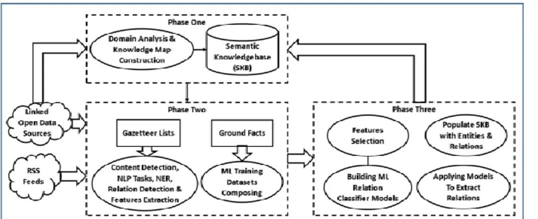
Our approach integrates domain knowledge with ML classification to improve the fundamental information retrieval tasks of Named Entity Recognition and Relation Classification. The approach is based on comprehensive analysis of the key concepts and relations of the targeted domain, which are modelled, using Semantic Web technologies, into a formal ontology that is used to semantically tag the entities and interrelations extracted from relevant Web documents. This effectively transforms the initial ‘conceptual’ domain knowledge into an enriched knowledgebase that can be intelligently explored by means of sophisticated interrogation of the integral and inferred facts within a single document or a set of interrelated documents [18]. The tasks of our approach are implemented in three main phases as depicted in Fig. 1, they are:

1) Phase one: Domain analysis and constructing the knowledge map and then translating it into a formal semantic model, ontology.

2) Phase two: Natural Language pre-processing tasks for Named Entity Recognition including, relation detection, features extraction and training datasets generation.

3) Phase three: Relation classification including features selection by utilising supervised ML and then inserting the semantically annotated information into semantic ontology.

The unstructured data source of this research is online financial news articles. They are retrieved by using the Rich Site Summary (RSS) feeds including BBC, Reuters and Yahoo Finance. For the purpose of training datasets generation, we retrieve 6135 documents from the online news RSS feeds. Table 1 presents some examples of those news RSS Feeds links.

TABLE 1: EXAMPLE OF RSS FEEDS

http://rss.cnn.com/rss/money_markets.rss

http://articlefeeds.nasdaq.com/nasdaq/categories?category=International

http://feeds.bbci.co.uk/news/business/rss.xml http://feeds.reuters.com/reuters/UKPersonalFinanceNews https://uk.finance.yahoo.com/news/provider-yahoofinance

Building the domain’s knowledge map aims to create a prearranged vocabulary and semantic structure for exchanging information about that domain. We modelled the domain knowledge in terms of the problem (use case) domain’s key concepts, their interrelations and the characteristics of the data as well as the interaction with the target beneficiary groups. Then, the knowledge map is translated into a formal semantic model, ontology. The ontology can be utilised to source knowledge from publicly available datasets that are published using the same standardised formalism. Moreover, ontology reasoning can infer more information about knowledge facts in different contexts [18]. As shown in Fig. 2 the target domain knowledge is structured as a map of interrelated concepts that can be easily revised and improved by both the domain experts and knowledge engineers.

Fig. 2: The concept Map of this work

The following subsections describe in detail the pre-processing tasks for our proposed hybrid relation classification approach.

(4)

A. Relation Detection

Our relation extraction approach is implemented at the sentence-level. Every entity pair for a targeted relation that appears in a sentence in unstructured data is identified and annotated as a relation instance and is assumed to represent one relation type. Relation detection grammar rules are encoded using GATE’s pattern matching language JAPE (Java Annotation Patterns Engine) [19]. The number of detected sentences and relation instances of the targeted relations in this work is shown in Table 2. These relation instances will be used to compile the relation classification’s training datasets.

TABLE 2: SENTENCES AND NUMBER OF PAIRS OF RELATION INSTANCES

Annotation Type Number

Sentences 251237

Relation Instances of Person-Organisation pairs 26316 Relation Instances of Person-Location pairs 31012 Relation Instance of Location-Organisation pairs 22567 Relation Instances of StockSymbol-Organisation 1174 Relation Instances of StockIndex-Organisation 777 Relation Instances of Organisation-Percent 5213 Relation Instances of StockIndex-Percent 1761

B. Feature Extraction

We argue that domain knowledge can assist in selecting the relation classifiers’ features vector. Therefore, we exploit the semantic knowledge of the problem domain to extract new features that expand on the features set used in traditional ML relation classification efforts such as that by Mintz, et al. in [20]; for instance, we added dependency paths and entity description features. As the dependency path (grammatical relation) between the related entities is not always apparent, we took into consideration the dependency paths of all words in the sentence including the candidate relation entities. The entity description features include its Parts of Speech annotation, the entity string and the number of words in the entity.

The features are categorised into three categories, Lexical features, Syntactic Features and Named Entity Features as illustrated in Table 3 below. These features are extracted by using JAPE rules in the GATE Embedded framework and added to every relation instance in the unstructured data.

TABLE 3: ML FEATURES VECTOR LIST (LEX=LEXICAL, SYN=SYNTACTIC & ENT=NAMED ENTITY FEATURES CATEGORY),

Cat. Name Description

Lex poslist

POS of words between entity pairs. A specific class of POS such as “JJS”, the superlative adjective ending with “est”

genposlist

General POS of words between entity pairs. A generic class of POS such as “JJ”, any adjective form.

posbefore POS of three words before the left entity posafter POS of three words after the right entity. posentity1 POS of the first entity

posentity2 POS of the second entity

Syn

dependency-Path

The whole collapsed typed dependency path of the entity pairs’ sentences. It is the path of the grammatical relations hold between all pairs of words in a sentence such as adjectival complement (acomp) relation between a verb and an adjective.

dependency-Kinds

The kinds of collapsed typed dependency path between entity pairs

dependency-Word

The words’ strings of collapsed typed dependency path between entity pairs.

directDep Direct collapsed typed dependency path between entity pairs

wordsStrSeq The strings of the words between entity pairs depDistance The number of the collapsed typed dependency

between words

Ent

enttokensno1 The number of tokens in the first entity enttokensno2 The number of tokens in the second entity order The order of the entities

distance The number of tokens between the two entities entityString1 Token string of the first entity

entityString2 Token string of the second entity typeentity1 The type of the first entity typeentity2 The type of the second entity

IV.ML-BASED RELATION CLASSIFICATION

Selecting an appropriate ML algorithm depends on the problem specification and the nature of the data [21]. We implemented and evaluated three different supervised ML relation classifiers, Support Vector Machine (SVM), Perceptron Algorithm Uneven Margin (PAUM) and K-Nearest Neighbour (KNN). The works of Li, et al. in [22], Piskorski, et al. in [23] and Witten, et al. in [24] reveal that these algorithms are used in IE tasks with adequate results.

SVM is a supervised ML algorithm that has proved effective for a diversity of classification tasks including many IE tasks. The most important parameters of this implementation are SVM cost (C, the Cost associated with allowing training errors, soft margin) and the uneven margins ( or tau, setting the value of uneven margins parameter of the SVM) [22] [25].

PAUM is a simple and effective learning algorithm especially for large training datasets. It has been successfully used for document classification and IE. It has three parameters, positive (p) and negative (n) margins, which allow the PAUM to handle imbalanced datasets better, and the modification of the bias term parameter (optB) [26]. KNN uses simple techniques and its accuracy is often enhanced when the number of features is small; the KNN implementation used in this work has only one parameter, K [27].

This work uses the GATE implementation for the three ML algorithms above as explained in the work of Cunningham, et al. in [8].

The algorithms above can implement both binary and multi-class classifiers. Multi-classification is usually solved in terms of multiple binary classifications by using a simple “one-vs-others” or “one-vs-another” models [22]. Rifkin, et al. in [28] argue that the “one-vs-others” approach is simple, robust and the accuracy of its results is better or similar to other approaches such as the single machine and error-correcting coding approaches besides that it requires less number of models. For these reasons, a number of studies have employed this multi-class approach; for example, the work of Archibald, et. al in [29] and the work of Chandrashekar, et. al in [10]. Hence, we adopted the “one-vs-others” method to transform multi-classifier into multiple binary.

The key elements affecting the accuracy of supervised ML algorithms are the training datasets, the feature vector and the learning model parameters. The configuration of these elements affects the accuracy of algorithms’ results. The next subsections present how we generated the training datasets, tuned the algorithms’ parameters and selected the best feature subsets for relation classification.

A. Generating the Training Datasets

We adopted two methods to generate the labelled instances for the training datasets, using manual annotation and automatically by means of extracting ground facts from existing public datasets.

(5)

1) Generating training datasets from online structured datasets

We have employed Semantic Web technologies to model our problem domain knowledge and subscribe the retrieved data to it using the Resource Description Framework (RDF) standard. The same standardised metadata is used in public datasets in the Linked Open Data (LOD) Cloud to publish ground facts that are relevant to various problem domains. These ground facts can be used to compile training datasets for relation classification and enriching the resulting knowledgebase. Hence, we adopted a knowledge-driven distant supervision ML approach to extract common entity pairs’ relations by utilising two existing knowledge datasets as a distant supervision sources for ML relation classification. These datasets are DBpedia2_{and Freebase}3_.

At the time of writing this document, DBpedia contained more than 4.5 million entities and more than 3 billion RDF triples for a diversity of languages. Freebase dataset contained approximately 47.5 million topics and 2.9 billion facts in English language.

The training datasets were built by retrieving the relations between any two entities in a single sentence in the unstructured document that are mentioned in Freebase or DBpedia as ground facts. These relations are assumed to be a class instance or true positive in the training datasets. The mentioned relations in the semantic datasets were extracted by using JENA’s SPARQL engine. JENA4_{is a free and open}

source Java framework for building Semantic Web and Linked Data applications, and SPARQL5_{is an RDF Query}

Language recommended by W3C for interrogating semantic stores. The complete implementation details of this task were published in our previous paper [18].

2) Generating training datasets manually

Although manual annotation of ML relation instances is a labour-intensive task, it is generally considered to be more precise than automatic annotation. In this research, we applied manual annotation to generate training datasets to extract uncommon relations between pairs that could not be found in exiting semantic datasets, DBpedia and Freebase. We employed GATE annotation tools to extract the training

2 http://wiki.dbpedia.org/

3 https://developers.google.com/freebase/

instances for ML. Table 4 shows the three training datasets that were collected manually.

B. Parameters Optimisation

The optimisation of the ML algorithms’ parameters is the problem of choosing/tuning a set of parameters’ values that result in improving the ML classifiers’ performance by tuning the ML algorithms’ parameters.

Lorena, et al. in [30] report that there are generally three methods to find the ML algorithms’ parameters optima: use the default values, define the values by grid search and automatic search through optimization techniques such as GAs. Grid based search is commonly used to perform parameter optimization, where the default values for the ML algorithms’ parameters are evaluated against the other values in the grid. In this work, we adopted grid-based search to perform parameter tuning as it is sufficient to satisfy the requirements of the deployed ML techniques and is simple to implement in comparison with the computationally expensive automatic optimisation techniques [31].

Practically, grid search starts with a finite set of reasonable values for each parameter. These values are selected manually in accordance with the specifications of each algorithms. Then, the selected grid sets are used to train the ML algorithms and evaluate their performance against ground-truth in a k-fold validation process. Finally, the parameters that achieve the highest model performance are chosen [32][31]. In this work, the finite sets of parameter values for SVM and KNN (paramxeters C and tau for SVM, K for KNN) were heuristically selected by studying the specifications and recommendations of those algorithms. However, for the PAUM algorithm parameters (p, n and optB), we relied on the recommended parameters’ values by the work of Li, et al in [33]. The parameters’ values selected by grid search proved favourable to the traditionally accepted default values for the SVM, PAUM and KNN algorithms. Table 5 shows the parameters of SVM, PAUM and KNN that were selected using the grid search experiments.

V. OPTIMISING FEATURE SELECTION USING GENETIC ALGORITHMS

The features in the solution space for Relation Classification are loosely related, which makes the utilisation of manual search techniques difficult. Hence, we automate the feature selection process by applying Genetic Algorithms search in a wrapper approach. In the wrapper approach, the classifier model itself is employed to measure the fitness of features set; in other words, the features selected depend on the classifier model used.

4 https://jena.apache.org/

5 https://www.w3.org/TR/sparql11-overview/ TABLE 4: THE SUMMARY OF THE COLLECTED TRAINING DATASETS

(RI=ALL RELATION INSTANCES, RC= RELATIONS CLASSES, DOC=DOCUMENTS, P=PERSON, O=ORGANISATION, L=LOCATION, S=STOCK SYMBOL, I=STOCK INDEX, C=PERCENTAGE)

Pairs Method Doc RI RC Relation Types P-O Distant Supervision 161 4213 204

founderOf 38 keyPersonIn 107 employerOf 59 P-L Distant Supervision 636 1115 2 896 hasPlace 221 birthplace 233 hasNationality 415 deathPlace 27 L-O Distant Supervision 281 6217 299 locatedIn 299 S-O Distant Supervision 71 316 83 issuedBy 83 I-O Manual 44 -- 107 memberOf 107

O-C Manual 399 -- 753

shareIncreasedBy 257 shareDecreasedBy 259 profitIncreasedBy 155 profitDecreasedBy 82 I-C Manual 91 -- 234 indexIncreasedBy 115

indexDecreasedBy 119

TABLE 5: THE GRID SEARCH RESULTS OF OPTIMUM ML ALGORITHMS PARAMETERS

ML P Grid

Result Description

SVM C 1

The Cost associated with allowing training errors (soft margin)

tau 0.8 Setting the value of uneven margins PAUM

p 10 Positive margin n 1 Negative margin

optB 0.3 The modification of the bias term KNN K 1 The number of nearest neighbour instances

(6)

We have adopted the conventional implementation of GAs that generally comprises the initialisation of the solution space population, population reproduction, crossover and mutation operations and defining the fitness function for evaluation. However, several techniques can be deployed to implement the aforementioned operations; for instance, there are two techniques for population reproduction, steady-state and generational populations and there are several methods for the population initialisation such as randomness, compositionality and non-compositionality. Similarly, parent selection can be performed using Stochastic Universal Sampling (SUS) or the Roulette Wheel Selection (RWS), and parent replacement can be based on the replacement of the worst parent or the replacement of random parents. The crossover operation could be applied to one or two crossover points in the chromosome and mutation operation could be applied on one or more genes in the chromosome [34][35][36]. We conducted a series of experiments to heuristically determine the techniques that represent a better fit for our feature selection problem.

In our implementation, the genetic-information or chromosome is represented by a binary string of 1’s and 0’s (genes) that operate as a feature filter, where every bit or gene in the chromosome represents a certain feature. If the bit value equals one, this means that its feature is selected to participate in constructing the classifier model, otherwise the feature must be removed. The size of the features vector in this work is 20, which means that the size of the chromosome is 20 bits. Fig. 3 shows how the chromosome filtering is working.

Fig. 3: Chromosome features filtering

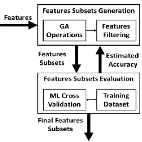
For the purpose of using GA as a wrapper approach, the ML classifiers are utilised to assess features’ subsets according to their classification performance. In detail, we define the fitness function using the classification F1 score, which is computed by evaluating the relation classification model using k-fold Cross Validation. The fitness values are computed as follows:

1) By filtering a specified chromosome, a feature subset is generated to train the relation classification model.

2) The generated feature subset is evaluated by applying k-fold Cross Validation on the classification models with the targeted training dataset and feature subset as an input. 3) The resulting F1-score is assumed to be the fitness function value for the specified chromosome or feature subset.

Fig. 4 below illustrates the workflow of the features selections process as wrapper approach.

By means of experimentation, we heuristically selected the Roulette Wheel technique for parent strings selection and adopted two-points and all points for the crossover and mutation operations respectively. For population initialisation, we adopted randomness initialisation. There are two techniques for population reproduction, steady state and generational techniques. We adopted the steady state

technique with the unconditional replacement of the worst chromosome for the parent replacement strategy because it is commonly used to assist in improving the performance of GAs. Steady state technique is less computationally intensive than generational technique; for instance, for 20 population size and two parent selection and 50 iteration, it requires 120 fitness calls instead of 1100 fitness calls for generational technique.

Fig. 4: GA feature subsets selection as Wrapper Approach

GAs have their own parameters that require more experimentation to find the best fit for a specific optimisation problem. These parameters are, initial population size, the number of generations, crossover rate and mutation rate. These parameter values should be adjusted for each problem because they would be related to characteristics of the problem. Small population size might not provide a sufficient sample size for the search space in order to reach an optimum solution. On the other hand, a large population requires more evaluations per generation, which can result in a slow rate of convergence. The crossover rate controls the frequency of applying the crossover operator on the selected parents to generate offspring. The higher the crossover rate, the more quickly new solutions are introduced into the population. If the crossover rate is too low, the search might be inactive due to the lower exploration rate. Similarly, the mutation rate controls the frequency of applying the mutation operator on the selected parents after applying crossover operator to increase the variability of the population. A low level of mutation rate serves to prevent any given gene position in the chromosome from converging to a single value in the entire population. A high level of mutation yields an essentially random search. Lastly, we needed to determine the optimal number of generations as it is directly related to the number of evaluations or fitness functions calls and hence impacts the efficiency of the GAs implementation. By means of experimentation, we heuristically established the parameters that represent the best fit for our feature selection problem. The values of the parameters are shown in Table 6.

TABLE 6: OUR IMPLEMENTATION OF GAS PARAMETERS

Parameters Values

The number of generations 100

The population size 20

The crossover rate 0.6

(7)

Our implementation of Genetic Algorithm operation steps to select the best features subset are as in the following Pseudo-code:

Algorithm 1: Genetic Algorithm Implementation

1: Start:

2: N is the size of the population

3: Pc is the crossover rate and Pm is the mutation rate 4: Let the best solution S*_{and its fitness F}*_(S*_{) equal to 0}

5: Generate initial N chromosomes Ci for the initial

Population, where i ∈ [0,1,…,N)

6: Evaluate initial chromosomes Ci, to be of finesses F(Ci);

7: repeat

8: Apply Roulette Wheel tech. to select two parents’

chromosomes, Cj and Ck,where 0 ≤ j,k < N and j≠k

9: Generating new chromosomes

10: Apply two points crossover operation on Cj and Ck

chromosomes with probability Pc

11: Apply all points mutation operation on Cj and Ck

chromosomes with probability Pm

12: Let new chromosomes be Cj’ and Ck’, children’s

chromosomes

13: Evaluate Cj’ and Ck’, the fitness of the children’s

chromosomes are F(Cj’) and F(Ck’)

14: Unconditionally replace children’s chromosomes Cj’

and Ck’ with the worst chromosomes in population

15: Find best chromosome Cb with best fitness F(Cb) in

the current population, where 0 ≤ b< N

16: Let the current solution S equals the best chromosome

Cb and the current fitness F equals F(Cb)

17: if F > F*_then

18: Update the best solution and the best fitness; 19: S*_{=S ;}

20: F* _{= F ;}

21: end if

22: until (stopping condition is met) 23: Return S*_{, F}*

24: End

Our implementation of GAs’ operations output is the chromosome that has best fitness value in the population. The selected features of this chromosome are considered to be the best for the targeted classifier model. More details about our evaluation results are presented in the ensuing section.

VI.EVALUATION RESULTS AND DISCUSSION

There are two commonly used evaluation methods for ML algorithms, K-fold cross-validation and holdout test. In K-fold cross-validation, the corpus is split into K equal size partitions of documents. The evaluation run is repeated K times (folds). Each partition is used as test dataset and all the remaining partitions as a training dataset for all K folds. The overall Recall, Precision and F1-measure result of this method is the average of the all folds’ results. In contrast, in holdout test, a number of documents in the training datasets are randomly selected according to a specified ratio, the default is 66%. All other documents are assumed to be testing dataset [37][8]. In this work, we used cross validation K-Fold with K=10, which is empirically found to be the best method in practical ML evaluations as reported by Witten, et al. in [24].

There are two different options for computing precision, recall and F1-measure over a corpus: micro averaging and macro averaging. In micro averaging, the corpus is treated as

one large document, where True Positive, False Positive and False Negative are counted through the entire corpus, and precision, recall and F1-measure are calculated accordingly. On the other hand, macro averaging computes precision, recall and F1-measure by counting True Positive, False Positive and False Negative on every single document and then averages the results for the entire corpus [8]. Macro Averaging is more appropriate for our problem domain since the sourced financial news articles represent independent documents.

According to Witten, et al in [24], there is more than one method to plot the evaluation results of ML algorithms performance. These methods depend on the target domain. For instance, the marketing domain uses lift chart by plotting True Positive rate versus training subset size, the communication domain uses Receiver Operator Characteristic (ROC) curve by plotting True Positive rate versus False Positive rate and the Information Retrieval domain uses Recall versus Precision curve. This research computes the evaluation results of ML models in relation classification by drawing the relation between recall and precision in terms of the confidence threshold for classification or the threshold probability classification as it is commonly accepted as the standard in the Information Extraction field.

The probability threshold value is an important factor for the best classification results in the majority of Machine Learning classifiers. In these classifiers, a set of instances are assigned to a class if their probability of class membership is greater than a probability threshold ρ, where 0 ≤ ρ ≤ 1. For example, with the default probability threshold value of 0.5, the predicted probability value of any instance to be a member of a certain class as a true positive must be greater than 0.5 [38]. However, Freeman, et. al in [39] have asserted that the accuracy of the classification models is affected by the value of the threshold. They added that the default threshold value of 0.5 does not necessarily produce a highest prediction accuracy; particularly, when the datasets are highly imbalanced. It should be noted, however, that in all the previous studies in Relation Extraction that are reported in the open literature and to the best of authors’ knowledge, the impact of probability threshold values on the relation classification accuracy has not been given great attention by the researchers in the past. This motivated us to investigate the impact of the probability threshold in relation classification in our research by means of experimentation. We heuristically selected the best threshold value for all classification models on all training datasets by drawing on the correlation between the threshold probability classification and F1-measure.

As presented in section 4 and Table 4, we generated seven different training datasets that cover different relations between different entity concepts in the financial and economic news domain. The sources of the unstructured documents are RSS Feeds (see Table 1).

In the seven training datasets, all the named entities are automatically annotated; however, the classes’ relation instances are automatically annotated in four training datasets and manually annotated in the other three training datasets.

The ML relation classification models have been created by using the training datasets with the features vectors. These models should be evaluated before applying them to extract

(8)

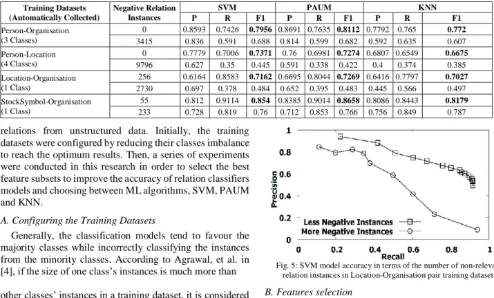
relations from unstructured data. Initially, the training datasets were configured by reducing their classes imbalance to reach the optimum results. Then, a series of experiments were conducted in this research in order to select the best feature subsets to improve the accuracy of relation classifiers models and choosing between ML algorithms, SVM, PAUM and KNN.

A. Configuring the Training Datasets

Generally, the classification models tend to favour the majority classes while incorrectly classifying the instances from the minority classes. According to Agrawal, et al. in [4], if the size of one class’s instances is much more than other classes’ instances in a training dataset, it is considered imbalanced. In our training datasets, specifically the datasets that are generated using public distant supervision sources (DBpedia and Freebase), the number of negative relation instances is large. This is attributed to the fact that some relations in our unstructured data will be incorrectly assumed to be negative instances as they are not included as ground facts in the sourced public datasets. We believe that these negative relation instances can disrupt the balance between True Positives and Negatives instances of the classes in the training datasets.

The first set of experiments attempts to alleviate the classes’ imbalance in terms of True Positive and True Negative numbers in order to improve the accuracy of the classification model and to speed up ML processing. In these experiments, we heuristically measure the impact of reducing the number of negative relation instances on the models’ accuracy by reducing or removing the relation instances in the documents that are not mentioned in the distant supervision sources. We also explicitly add some negative relation instances in the training datasets of one relation class in order to decrease in the true positive rate while maintaining a low false positive rate as recommended by Mohamed, et al. in [40]. Table 7 above shows the impact of reducing the number of negative Relation Instances on ML models’ accuracy in terms of Precision, Recall and F1-measure.

Mintz, et. al in [20] utilise multi-class logistic classification for relation extraction and reported that the negative relations instances had a minor effect on the performance of their classifier. However, for the implemented SVM classification, it is evident from Fig. 5 that the SVM model accuracy clearly improves as we reduce the number of the True Negative relation instances because the class distribution in the training datasets does play a major role in the performance of most classification algorithms as highlighted by Agrawal, et. al in [4].

Fig. 5: SVM model accuracy in terms of the number of non-relevant relation instances in Location-Organisation pair training dataset.

B. Features selection

The second set of experiments concerns feature selection by using GAs in a wrapper approach. First, we find the best subset of features by using our implementation of GAs, and then evaluate the relation classification models using the selected feature subset.

Fig. 6: The Genetic Algorithm Iterations to select the best feature subset for Stock Index and the Percentage increase or decrease training dataset

1) Feature selection results

Using the same parameters listed in Table 6, we execute our implementation of the GA. The results in Fig. 6 illustrate the required number of GAs’ iterations required by SVM, PAUM and KNN to select an optimal fitness function value (F1 measure); SVM, PAUM and KNN require 57, 54 and 69 iterations respectively. We conclude that the three ML algorithms require approximately the same numbers of iterations to reach the optimal fitness value and that 100 iterations are quite sufficient for the GAs to achieve that goal.

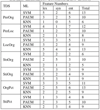
Table 8 below shows the number of selected features in every subset for every classifier, SVM, PAUM and KNN, in all training datasets. This table also shows the features in every subset, which are classified into the three categories, Lexical, syntactic and Named Entity category.

TABLE 7: SHOWS THE IMPACT OF REDUCING THE NUMBER OF NEGATIVE RELATION INSTANCES ON ML MODELS ACCURACY IN TERMS OF PRECISION, RECALL AND F1-MEASURE

Training Datasets (Automatically Collected) Negative Relation Instances SVM PAUM KNN P R F1 P R F1 P R F1 Person-Organisation (3 Classes) 0 0.8593 0.7426 0.7956 0.8691 0.7635 0.8112 0.7792 0.765 0.772 3415 0.836 0.591 0.688 0.814 0.599 0.682 0.592 0.635 0.607 Person-Location (4 Classes) 0 0.7779 0.7006 0.7371 0.76 0.6981 0.7274 0.6807 0.6549 0.6675 9796 0.627 0.35 0.445 0.591 0.338 0.422 0.4 0.374 0.385 Location-Organisation (1 Class) 256 0.6164 0.8583 0.7162 0.6695 0.8044 0.7269 0.6416 0.7797 0.7027 2730 0.697 0.378 0.484 0.652 0.395 0.483 0.445 0.566 0.497 StockSymbol-Organisation (1 Class) 55 0.812 0.9114 0.854 0.8385 0.9014 0.8658 0.8086 0.8443 0.8179 233 0.728 0.819 0.76 0.712 0.853 0.766 0.756 0.849 0.787

(9)

From the data in Table 8, it is apparent that the features of the Named Entities category are more important than the features of the lexical and syntactic categories in the majority of the training datasets. These results are consistent with the findings of Wang, et al. in [41] who noted that the entity features lead to improvement in performance because the mentioned relation between two entities is closely related to the entity types.

2) Evaluating the Relation Classification Models by using the Selected Feature subsets

The selected feature subsets in the training datasets are employed to create the relation classifiers’ models. These models are evaluated by using 10-fold cross validation. Table 9 shows the comparison between the F1-measures results of the three relation classifiers models, SVM, PAUM and KNN when they use all features vectors and when they use the feature subsets. Also, the table indicates the best F1-measure in terms of the best probability threshold.

Fig. 7 illustrates the impact of the probability threshold on the F1-measure upon SVM relation classification when using all the classification features and the features subsets selected by our implementation of GA. It is clear that the F1-measure peaks upon probability threshold of 0.4.

All of the classifiers that we studied, SVM, PAUM and KNN, performed significantly better in the reduced feature space optimised by the GA. As evident in Table 9, our implementation of GAs has improved the accuracy of ML algorithms in all training datasets. It can also be noticed that the improvements registered for SVM and PAUM are more evident compared to KNN. KNN is more sensitive to the irrelevant features, which is corroborated by Imandoust, et

al. in [42] while Wang, et al. in [41] assert that the mechanism of SVM learning makes the irrelevant features have little impact on the performance of the SVM algorithm.

Our experiments have also indicated that the accuracy of the classification models is affected by the value of the probability threshold. The best threshold values for all classification models on all training datasets were empirically selected to deliver better classification accuracy compared to the default threshold value 0.5 as evidenced in below.

Fig. 7: Impact of threshold on SVM relation classifiers’ accuracy

It can be observed from Table 9 that our implementation of GA selects features from the Named Entity category more frequently than from the lexical and syntactic categories for the majority of the training datasets. Consequently, we decided to conduct further research to investigate the impact of the features categories on the classifiers’ performance.

With respect to the performance of the SVM, PAUM and KNN relation classifiers, the data in Table 9 indicates that the accuracy of SVM classifier outperforms PAUM and KNN for most of the training datasets, which are Person-Organisation, Person-Location, StockIndex-Organzation and Organisation-Percent training datasets. The recorded results consistent with the findings of other studies that utilise ML in relation classification; for example, the study by Li, et al. in [43] found that SVM may perform better than PAUM in small training datasets and they have a close performance in large training datasets. Also, the work of Hmeidi, et. al in [27] reveal that SVM has better F1-measure results than KNN. We believe that PAUM and KNN exhibit better performance than SVM in some training datasets because PAUM is appropriate for imbalanced training datasets and KNN performs better with small number of features.

C. Features Category Selection

This section evaluates the effect of the features of a single category (Lexical, Syntactic or Named Entity) on the accuracy of the relation classification

models. We created the models by using training datasets with features of each category individually and with feature combinations of all categories. The models’ evaluation

TABLE 8: THE FEATURE SUBSETS THAT ARE SELECTED BY USING GAS (LEX=LEXICAL, SYN=SYNTACTIC & ENT=ENTITY) TDS ML Feature Numbers

lex syn ent Total PerOrg SVM 5 2 6 13 PAUM 3 2 5 10 KNN 1 0 5 6 PerLoc SVM 4 1 7 12 PAUM 1 2 7 10 KNN 2 1 5 8 LocOrg SVM 3 3 5 11 PAUM 3 2 4 9 KNN 5 4 4 13 StsOrg SVM 2 2 2 6 PAUM 2 5 3 10 KNN 2 1 2 5 StiOrg SVM 3 3 3 9 PAUM 3 2 4 9 KNN 5 3 1 9 OrgPct SVM 3 3 5 11 PAUM 2 5 6 13 KNN 2 2 5 9 StiPct SVM 1 3 4 8 PAUM 2 3 5 10 KNN 2 3 4 9

TABLE 9: COMPARING THE CLASSIFIERS RESULTS IN TERMS OF F1 SCORE BEFORE AND AFTER GAS RESULTS (THR=PROBABILITY THRESHOLD, ALL=F1 WHEN ALL FEATURES, GA=F1 WHEN FEATURES SELECTED BY GA)

Entity Pairs Type SVM PAUM KNN

Thr. ALL GA Thr. ALL GA Thr. ALL GA

Person-Organisation 0.5 0.7956 0.825 0.65 0.8072 0.8125 0.5 0.772 0.8111 Person-Location 0.4 0.736 0.7564 0.65 0.7278 0.7514 0.7 0.668 0.7321 Location-Organisation 0.55 0.7236 0.7344 0.5 0.7269 0.7577 0.8 0.7045 0.7489 StockSymbol-Organisation 0.55 0.8689 0.8643 0.5 0.8583 0.8689 0.5 0.8179 0.8768 StockIndex-Organisation 0.6 0.8548 0.8898 0.5 0.8765 0.8771 0.4 0.8449 0.8774 Organisation-Percent 0.15 0.6513 0.6715 0.15 0.6463 0.6649 0.8 0.58 0.6443 StockIndex-Percent 0.4 0.7032 0.7726 0.5 0.7268 0.7804 0.5 0.7052 0.7622

(10)

results are compared in Table 10. The data in the table indicates that the best Precision, Recall and F1-measure values are produced when features of named entities category are included in the training.

The results of these experiments illustrate that the models that are created using the Named Entity category combined with lexical and/or syntactic features, exhibit better accuracy than the models created without including the Named Entity category. This is true for the all training datasets and all ML classifiers except the training dataset of the relation between Stock Symbol and Organisation entities when using SVM and PAUM classifiers. This is attributed to the fact that the relation instance correlating Stock Symbol and Organisation is short in terms of the number of words (sometimes there are no words between the entity pairs) compared to other relations (with more than two words between the entity pairs). This reduces the effectiveness of certain features; for instance, the features that represent the number of tokens between the entities in the relation instances and the features that represent the POS of the words between the entities. Table 11 below illustrates the difference in POS features for StockSymbol-Organisation and Organisation-Percent relation instances.

TABLE 11: EXAMPLES OF THE POS FEATURE OF TOKENS BETWEEN ENTITY PAIRS

Relation Instance

Example Entity 1 Entity 2

POS feature of tokens between entity pairs Axalta Coating Systems Ltd. (AXTA Axalta Coating Systems Ltd. AXTA

There is only one token between the two entities. It is the right brackets “(“ Apple were crushed again Friday, falling $6.60, or 5.86% Apple 5.86% VBD-VBN-RB-NNP-,-VBG-$-CD-.-CD-,-CC

The number of POS tokens between the entity pairs in the relation instance of StockSymbol-Organisation training dataset is only one and the number of POS tokens between the entity pairs in the relation instance of and Organisation-Percent training dataset is 12. It is clear that the features which are related to the tokens between the entity pairs in the StockSymbol-Organisation training dataset are not sufficient to indicate the syntactic relation between organisation and its stock symbol within the context.

In general, the classification accuracy of the ML models has improved as a result of deploying our GA for optimising the feature selection process. In section 7, we further assert this claim by comparing it against another solution search method for features selection.

VII. CONTRASTING OUR IMPLEMENTATION OF GA

OPTIMISATION TO RANDOM MUTATION HILL-CLIMBING

In this section, we attempt to verify that GAs are an appropriate choice for optimising the process of features selection for the relation classification problem. Hence, we decided to compare our implementation of GAs with Random Mutation Hill-Climbing (RMHC) as their operational dynamics are very similar. Our choice of HC to compare against GAs for the feature selection optimisation problem is consistent with numerous studies that elected to compare between the two algorithms, for a variety of problems, since their early conception. One of the earliest investigations was carried out by Mitchell, et al. in (Mitchell et al. 1994) who attempted to answer the question: when will a GA outperform Hill-Climbing? They claim that understanding the mechanism of GAs and the characteristic of the fitness landscapes of the problem is crucial for deciding when the GAs will be most useful. Another study by MacFarlane, et al. in [44] compared GAs to several types of HC algorithms including RMHC. The algorithms were applied to solve term selection problem for an information filtering task. Although they observed that both Genetic and Hill-Climbing algorithms appear to be able to improve accuracy of term selection, they did not find evidence that their implementation of GA performs better than that for their Hill-Climbing algorithm. A recent study by Sakamoto, et al. in [45] elected to compare GAs and HC in a completely different problem domain, which is simulating the node placements problem for achieving the network connectivity and user coverage.

RMHC can be considered as a GA without crossover operation and initial population. The solution neighbour or the new solution in RMHC can be generated by applying a similar mutation operation as in GAs, which could make jumps of varying sizes through the search space [36]. The other reason of choosing RMHC to compare with our implementation of GAs is to compare between the complexity of GA with the simplicity of RMHC and

TABLE 10: SVM, PAUM AND KNN CLASSIFIERS WITH CATEGORIZED FEATURES (FC=FEATURES CATEGORY, L=LEXICAL FEATURES, S=SYNTACTIC FEATURES, E=NAMED ENTITY FEATURES, THR=PROBABILITY THRESHOLD, P=PRECISION, R=RECALL, F1=F1 SCORE)

TDS SVM PAUM KNN

FC P R F1 Thr FC P R F1 Thr FC P R F1 Thr

PerOrg L+E 0.9052 0.7516 0.8194 0.55 L+E 0.8481 0.7868 0.8149 0.65 L+E 0.823 0.7788 0.7998 0.75 PerLoc E 0.7622 0.7266 0.7439 0.4 S+E 0.768 0.7014 0.733 0.65 E 0.7225 0.6951 0.7085 0.55 LocOrg E 0.6535 0.8645 0.7426 0.55 E 0.6893 0.8349 0.7526 0.5 E 0.7026 0.7804 0.738 0.75 StsOrg L 0.8796 0.9114 0.8914 0.5 L+S 0.8489 0.9114 0.8764 0.5 L+E 0.8518 0.8486 0.8433 0.9 StiOrg L+E 0.8114 0.9408 0.8664 0.65 L+S+E 0.799 0.9789 0.8766 0.5 S+E 0.7994 0.9292 0.8546 0.3 OrgPct S+E 0.6955 0.6419 0.6674 0.4 S+E 0.6811 0.624 0.6507 0.15 S+E 0.6158 0.6115 0.6136 0.5 StiPct S+E 0.6921 0.6921 0.6921 0.5 L+S+E 0.73029 0.721 0.7268 0.5 L+S+E 0.7281 0.6863 0.7052 0.5

(11)

answering the question: do we need the computational complexity of GA operations?

In our RMHC implementation, we adopted a similar configuration to that used by Sakamoto, et al. in [45]. The RMHC implementation works as in the following pseudo-code:

Algorithm 2: RMHC implementation

1: Start

2: Generate an initial solution S0;

3: Evaluate the initial solution S0, F(S0);

4: Let the current solution S equals the initial solution S0;

5: Let the best solution S*_{equals the initial solution S}₀_;

6: Let the best fitness value F* _{equals the fitness of the}

initial

solution F(S0);

7: repeat

8: Mutate current solution S to generate a new solution

S’;

9: Evaluate the new solution F(S’);

10: if F(S’) > F(S*_{) then}

11: Update the best solution and the best fitness; 12: S*_{=S’ ;}

13: F* _{= F(S’) ;}

14: end if

15: Update the current solution S = S’ ;

16: until (stopping condition is met) 17: Return S∗_{, F}∗

18: End

In order to fairly compare the performance of our implementation of GAs and RMHC for features selection problem, the experiments should be under the same computational conditions, in particular with respect to the fitness evaluation calls as it represents the most critical operational step of search algorithms. It is clear that one run of GAs is more expensive than one run of RMHC in terms of fitness functions calls [46]. As a result, we should run both algorithms with equal number of fitness function calls.

Because we adopted the steady state technique for population reproduction in our implementation of GAs, the number of fitness function calls will be equal to 𝐼 × 2 + 𝑃, where, I is the iterations number of GAs’ operations and P is the population size. However, the number of fitness function calls in RMHC is equal to the number iterations of its operations because our implementation of RMHC does not have initial population. Consequently, the number of iterations of RMHC experiments should be equal to the number of our GA fitness function calls.

For the purpose of this experimental comparison, we evaluate optimising the accuracy of the SVM relation classifier for only one training dataset (Location-Organisation). The number of iterations in our implementation of the GAs is 50, thus the algorithm makes 120 fitness function calls for a population size of 20; consequently, the Random Mutation Hill-Climbing algorithm should have 120 iterations in order to subject it to the same computational efforts in terms of fitness evaluations. The number of executed runs for each algorithm is 30, which represent the number of sample runs.

The comparison between our implementation of Genetic and Random Mutation Hill Climbing algorithms are highlighted in Table 12 in terms of fitness sample runs, i.e. F1-measure. The results in the table indicates that Random

Mutation Hill-Climbing algorithm outperforms our implementation of Genetic Algorithms in only 4 of the 30 sample runs.

From the data in Table 12, it is apparent that our implementation of Genetic Algorithms outperforms Random Mutation Hill-Climbing algorithm in most the results’ sample runs as our implementation of Genetic Algorithms have higher ranking sample runs than the sample runs of Random Mutation Hill-Climbing algorithm. Nevertheless, in order to further examine any significant difference in the performance of our implementation Genetic Algorithms and Random Mutation Hill-Climbing algorithm, we applied a statistical test to compare their performance in the feature subset selection problem. We considered a Wilcoxon singed rank test procedure to perform a pairwise comparison between the two algorithms’ sample runs. Wilcoxon test is a non-parametric statistical procedure for examining the median differences in observations for two samples. It aims to detect if there is a significant difference among the behaviour of the samples of two algorithms’ results. Before applying the Wilcoxon procedure test, we should rank the absolute differences of the two sample pairs. First, finding out the difference between each sample pair. Then, the absolute differences of the samples are ranked by ordering them from the smallest to the largest. The rank will be according to the position of the absolute difference of the pair in the ordered list [47]. Table 12 shows the fitness values for the sample runs of Genetic and Random Mutation Hill-Climbing algorithms; also, their paired sample runs differences and the ranks and total ranks of their absolute differences.

TABLE 12: GA AND RMHC F1-MEASURE SAMPLE RUNS AND THEIR ABSOLUTE DIFFERENCES RANKS

Sample Run # GA F1 RMHC F1 Difference GA Ranks RMHC Ranks 1 0.7460218 0.735 0.0110218 26 2 0.7368624 0.7319737 0.0048887 12 3 0.738097 0.7338212 0.0042759 6 4 0.7448637 0.7402726 0.0045911 10 5 0.7361086 0.728381 0.0077276 21 6 0.7298968 0.7381135 -0.0082167 22 7 0.7359173 0.7313907 0.0045266 8 8 0.7370021 0.7309848 0.0060174 17 9 0.7419199 0.7394984 0.0024215 3 10 0.7452387 0.7305558 0.0146829 29 11 0.7377635 0.7325595 0.005204 13 12 0.7390769 0.7343243 0.0047526 11 13 0.7368212 0.7398594 -0.0030382 5 14 0.7368653 0.7304085 0.0064568 19 15 0.7397724 0.7376058 0.0021667 2 16 0.7347115 0.7289391 0.0057724 16 17 0.7364395 0.7203119 0.0161276 30 18 0.7419509 0.7420638 -0.0001129 1 19 0.7370386 0.7249938 0.0120448 28 20 0.7394399 0.7287488 0.0106911 25 21 0.7457602 0.7364889 0.0092713 23 22 0.7398368 0.7299845 0.0098523 24 23 0.7423382 0.7304239 0.0119143 27 24 0.7362633 0.7423339 -0.0060706 18 25 0.7341355 0.728746 0.0053895 14 26 0.7377205 0.7304985 0.007222 20 27 0.7303425 0.725773 0.0045694 9 28 0.7415834 0.7371815 0.0044019 7 29 0.7321383 0.7292429 0.0028955 4 30 0.7438176 0.7381317 0.0056859 15 Total Ranks: 419 46