Bayesian Hierarchical Models for Model Choice

(1)

Bayesian Hierarchical Models for Model Choice

by

Yingbo Li

Department of Statistical Science Duke University

Date:

Approved:

Merlise A. Clyde, Supervisor

James O. Berger

Edwin S. Iversen

Elizabeth R. Hauser

Dissertation submitted in partial fulfillment of the requirements for the degree of Doctor of Philosophy in the Department of Statistical Science

in the Graduate School of Duke University 2013

(2)

Abstract

Bayesian Hierarchical Models for Model Choice

by

Yingbo Li

Department of Statistical Science Duke University

Date:

Approved:

Merlise A. Clyde, Supervisor

James O. Berger

Edwin S. Iversen

Elizabeth R. Hauser

An abstract of a dissertation submitted in partial fulfillment of the requirements for the degree of Doctor of Philosophy in the Department of Statistical Science

in the Graduate School of Duke University 2013

(3)

Copyright c 2013 by Yingbo Li

(4)

Abstract

With the development of modern data collection approaches, researchers may collect hundreds to millions of variables, yet may not need to utilize all explanatory variables available in predictive models. Hence, choosing models that consist of a subset of variables often becomes a crucial step. In linear regression, variable selection not only reduces model complexity, but also prevents over-fitting. From a Bayesian perspective, prior specification of model parameters plays an important role in model selection as well as parameter estimation, and often prevents over-fitting through shrinkage and model averaging.

We develop two novel hierarchical priors for selection and model averaging, for Generalized Linear Models (GLMs) and normal linear regression, respectively. They can be considered as and-slab” prior distributions or more appropriately “spike-and-bell” distributions. Under these priors we achieve dimension reduction, since their point masses at zero allow predictors to be excluded with positive posterior probability. In addition, these hierarchical priors have heavy tails to provide robust-ness when MLE’s are far from zero.

Zellner’s g-prior is widely used in linear models. It preserves correlation structure among predictors in its prior covariance, and yields closed-form marginal likelihoods which leads to huge computational savings by avoiding sampling in the parameter space. Mixtures of g-priors avoid fixing g in advance, and can resolve consistency problems that arise with fixed g. For GLMs, we show that the mixture of g-priors

(5)

using a Compound Confluent Hypergeometric distribution unifies existing choices in the literature and maintains their good properties such as tractable (approximate) marginal likelihoods and asymptotic consistency for model selection and parameter estimation under specific values of the hyper parameters.

While theg-prior is invariant under rotation within a model, a potential problem with the g-prior is that it inherits the instability of ordinary least squares (OLS) estimates when predictors are highly correlated. We build a hierarchical prior based on scale mixtures of independent normals, which incorporates invariance under ro-tations within models like ridge regression and the g-prior, but has heavy tails like the Zeller-Siow Cauchy prior. We find this method out-performs the gold standard mixture of g-priors and other methods in the case of highly correlated predictors in Gaussian linear models. We incorporate a non-parametric structure, the Dirichlet Process (DP) as a hyper prior, to allow more flexibility and adaptivity to the data.

(6)

(7)

List of Tables

2.1 Three commonly used distributions in the exponential family . . . 10

2.2 For GLMs: methods to be compared . . . 36

2.3 GLM simulation: four scenarios of true models . . . 39

2.4 Logistic regression: model selection accuracy under 0-1 loss. . . 41

2.5 Poisson regression: model selection accuracy under 0-1 loss . . . 42

2.6 Logistic regression: median SSE in estimation . . . 43

2.7 Poisson regression: median SSE in estimation . . . 44

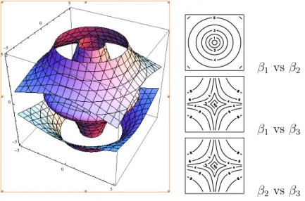
2.8 Pima Indian diabetes data: marginal posterior inclusion probability . 45 3.1 3D Contour plots of pβ1, β2, β3q . . . 56

3.2 Simulation of normal means case: median L2 loss in estimation . . . . 64

3.3 Simulation of normal means case: median L1 loss in estimation . . . . 66

3.4 Simulation of regression: median L2 loss in estimation . . . 68

3.5 Simulation of regression: marginal inclusion probability of LoRI . . . 69

(12)

List of Figures

3.1 Contour plots of logppβ1q versus logppβ2q . . . 53

3.2 Simulation of normal means case: shrinkage plots . . . 65

3.3 Simulation of regression: pairwise posterior probability . . . 70

3.4 Protein activity data: correlation among predictors . . . 72

3.5 Protein activity data: posterior results of LoRI . . . 73

(13)

Acknowledgements

First, I am so grateful for my advisor Merlise Clyde, who has been extremely sup-portive to me over the years. She has everything a student could ask for in a mentor. I would like to thank her, for her patience and insights. She generously shares with me her experience and wisdom as a scholar, and encourages me to pursuit academic career. She also teaches me the rigorous attitude towards research. She sets a role model as an intelligent and knowledgeable scholar for me.

I would like to thank my committee members, Ed Iversen for introducing me to a colorful world of genetic research; thank Jim Berger and Beth Hauser for their insightful comments. I especially want to thank David Banks, a great mentor, for his generous help to both my research and job hunting. I would also like to thank Mine C¸ etinkaya-Rundel and Dalene Stangl, for their advice and help for my summer teaching. I am very thankful to Fan Li, for her valuable comments and ideas for both work and life. My further thanks go to my mentors at Avaya Labs, Lorraine Denby, Jim Landwehr and Pat Tendick. I learned a lot from them during my summer intern. I must also thank my English teacher, Diane Bryson, for her generous help with paper revising. I thank Andrew Cron, Cliburn Chan and Jacob Frelinger, for helping me implementing their HDPGMM model.

This research was supported by the National Science Foundation grant DMS-1106891. I thank the National Science Foundation (NSF) and the Statistical and Applied Mathematical Science Institute (SAMSI) for their financial support to my

(14)

graduate study.

I feel so fortunate to have made friends with a lot of kind and smart people, especially, Hongxia, Minhui, Jianyu, Fangpo and Monika. I learn from them and enjoy their company.

Last but not least, I would like to thank my parents and my husband. I am thankful to my parents, Guangsu Li and Juhong Ying, for their unconditional love and support. I am also very thankful to my husband, Qiang Wang, who makes me want to be a better person. I love you, too.

(15)

1

Introduction

In linear regressions, variable selection is routinely used to reduce model complexity and prevent over-fitting. From a Bayesian perspective, model selection is driven via prior specifications. In this dissertation, we develop two novel hierarchical priors for variable selection and model averaging. This chapter is organized as follows. Section 1 introduces the background of Bayesian model selection and model averaging in normal linear models. Section 2 describes the “spike-and-slab” prior, the class of prior distributions that contain point masses at zero as mixture components. Sections 3 and 4 review two widely utilized prior distributions, mixtures ofg-priors and scale mixtures of independent normals respectively. Overviews of our new methods are included in these two sections.

1.1 Background: Bayesian Model Selection and Model Averaging in

Linear Regression

From a model selection prospective, suppose we have pq pq number of potential predictors, among which the first q ones X0 pX0,1, . . . ,X0,qq should always be

(16)

(e.g. intercept); while a subset of the remaining ppredictors V pV1, . . . ,Vpqmay

be redundant or null predictors and may be excluded. We denote a normal linear regression model with predictorspX0,VMqas model M, which can be written as

ModelM: Y X0α0 VMβM , Np0, σ2Inq (1.1)

where Y py1, . . . , ynqT is the vector of n independent responses, and VM is the

design matrix that consists of certain pM columns ofV.

Bayesian solutions to the model selection problem require prior specifications on the model space, ppMq, and also on the parameters ψM pα0,βM, σq. After the

prior specification, for each model M, its marginal likelihood fpY | Mq and its posterior probabilityppM|Yq can be computed as

fpY |Mq

»

fpY|ψM,Mq ppψM |Mq dψM

ppM|Yq ° fpY|MqppMq M1fpY|M1q ppM1q

A widely used selection criterion is to select the model with the highest posterior probability ppM | Yq. In addition, model posterior probabilities also serves as weights in Bayesian model averaging (BMA), which uses the weighted average of posterior mean estimates of coefficients given each model,

˜

βj

¸

M

ppM|Yq _Epβj |Y,Mq 1tXjPXMu

Therefore, for both model selection and parameter estimation, calculating marginal likelihoods fpY |Mq is essential.

1.2 Prior Distributions with Point Masses at Zero

For Bayesian model selection and model averaging, prior specification for parameters plays an important role. The “spike-and-slab” type of priors are popular choices for

(17)

regression coefficients. Originally, the spike-and-slab prior (Mitchell and Beauchamp, 1988) refers to a mixture distribution of a points mass at zero (the spike) and a uni-form distribution on a bounded interval centered at zero (the slab). This concept nowadays is usually used to describe a class of prior distributions that are mixtures of point masses at zero and continuous distributions or “spike-and-bell” priors. With the point masses, a subset of predictors can be excluded with positive probability, which can be treated as direct shrinkage to zero. The continuous components in the prior also pull the coefficients included in the model towards their prior cen-ters, which are usually zero, to achieve another layer of shrinkage. When dealing with high-dimensional data, in addition to the spike-and-slab type of priors, another class of prior distributions, continuous shrinkage priors are also widely adopted. The density functions of these priors have high peaks around zero (or even diverge at zero), which can impose heavy shrinkage on the coefficients towards zero but can-not strictly exclude predictors unless posterior mode estimates are used, or some additional decision theoratic approach is adapted.

1.3 The

g-prior and Mixture of

g-priors

Among the spike-and-slab priors, Zellner’s g-prior is a very popular choice. In the regression problem Y NpXβ, σ2Inq, when there is some information about the value of the coefficient β but little information about σ and the prior covariance of

β, Zellner (1986) proposes the g-prior on pβ, σq,

β |g, σN β0, gσ2pXTXq1

ppσq 9 1{σ

which incorporates the possible value of the coefficient through the prior mean β0. Since for variable selection problems, selecting variables X is equal to testing hy-potheses H0 : β 0 versus Ha : β 0, hence here the possible value of the

(18)

coefficient is β0 0. In the g-prior, the normal standard deviation σ typically has an improper diffuse prior. Improper priors introduce arbitrary constants into the marginal likelihoods generally leading to ill determined Bayes factors, which may invalidate model comparison based on Bayes factors. Hence Bayarri et al. (2012) proposes the Basic Criterion for priors in model selection, which suggests that all model specific parameters should have proper conditional prior distributions. Com-mon orthogonal parameters are exceptions, due to the cancellation of the vague constants in the Bayes factors (Berger et al., 1998).

It is convenient to consider an equivalent parameterization of model (1.1) so that the common predictors X0 and remaining model specific predictors are orthogonal for all models. To achieve orthogonality, in (1.1) we decompose VM by projecting it onto the hyper plane spanned by the columns of X0,

Model M: _EpYq X0α0 PX0VMβM pInPX0qVMβM (1.2)

X0α XMβM (1.3)

whereαα0 pXT0X0q1XT0VMβM is the parameters on common predictors after

translation, PX0 X0pX

T

0X0q1XT0 is the projection matrix, and

XM pInPX0qVM (1.4)

is the new model specific predictors such that

XT₀XM 0 (1.5)

Formula (1.5) implies that the parameters α and βM are orthogonal in the sense of

the information matrix ofpα,βMqbeing block diagonal. Note that the above

orthog-onality holds under all 2p _{models, so} _α _{can be considered as a common parameter}

among different models. In the special case where the only common predictor is the interceptX0 1n, in normal linear regression transformingVM toXMis equivalent

(19)

to centering the columns of VM. And after this orthogonalization, the intercept α

can be considered as the center ofY, which does not change with any specific model

M. Therefore, in linear models according to the most widely used version of the Zellner’s g-prior, the interceptαhas an improper flat prior (e.g., Liang et al. (2008), the null-based approach)

βM |g, σ,MN 0, gσ2pXTMXMq1

(1.6)

ppα, σ |Mq 9 1{σ (1.7)

This version of the g-prior has several ideal properties. The marginal likelihoods yielded by it are in closed form expression, and can be represented as simple func-tions of the coefficient of determination or R2_{. In addition, it maintains the same} correlation structure in the prior distribution as the likelihood and is invariant un-der orthogonal transformation of designs. However, choosing the value of the hyper parameter g is not straight-forward. Arbitrary values of g in the g-prior usually lead to the information paradox (Liang et al., 2008). In addition, Lindley’s paradox occurs when g is large, because the prior density is too flat and hence always favors the smaller model. To resolve these problems, fully Bayes approaches propose prior distributions on g, e.g. Zellner and Siow (1980), Liang et al. (2008), Maruyama and George (2011), Bayarri et al. (2012), Celeux et al. (2012), Ley and Steel (2012).

1.3.1 Overview of Chapter 2

New mixtures of g-priors have been extensively studied in linear models, however choice of prior distributions in Generalized Linear Models (GLMs) remains an open problem. In Chapter 2 of this thesis we extend mixtures of g-priors to Generalized Linear Models (GLMs) by assigning a conjugate prior, the Confluent Hypergeometric distribution, to the shrinkage factor ₁g_g. Our CH-g prior encompasses common mixtures ofg-priors in the literature such as the Hyper-g prior, and naturally extends them to be applicable in GLMs. Under a Laplace approximation, it yields marginal

(20)

likelihoods in computationally tractable forms. We demonstrate theoretically the asymptotic consistency for model selection and BMA estimation holds under the CH-g prior. With our default choice of hyper parameters, the CH-g prior satisfies the intrinsic consistency of Bayarri et al. (2012) implicitly. In addition, we illustrate its use in simulation and real examples.

1.4 Scale Mixtures of Independent Normals

In addition to mixtures of g-priors, shrinkage methods with continuous priors in the family of scale mixtures of independent normals (West, 1987) are also preva-lently used, for example, the relevance vector machine (Tipping, 2001), the Normal-exponential-gamma prior (Griffin and Brown, 2005), the Bayesian lasso (Park and Casella, 2008), (Hans, 2009), the Bayesian elastic net (Li and Lin, 2010) and the horseshoe (Carvalho et al., 2010). Under orthonormal designs, the (conditional) posterior mean of each regression coefficient may can be represented as the MLE multiplied by a shrinkage factor, which takes value between 0 and 1.

The posterior distribution under the g-prior inherits the instability of ordinary least square (OLS) estimate when the design matrix is nearly singular. Ridge regres-sion, lasso estimates or estimates under scale mixtures of independent normals are not as affected by the correlation among the predictors. Carvalho et al. (2010) claim that the horseshoe performs almost as well as the gold standard of Bayesian model averaging (BMA) under the Zellner-Siow prior for prediction. However, continuous priors cannot shrink coefficients to exact zeros, and lack selection procedures that can be validated by optimizing any loss function. On the other hand, “spike-and-slab” priors (Mitchell and Beauchamp, 1988; Ishwaran and Rao, 2005; Scott and Berger, 2006) allow coefficients to be exactly zero (so that they can be excluded from the model) by adding positive probability masses at zero to the priors. Our results sug-gest that scale mixtures of independent normals may out-perform the mixtures of

(21)

g-priors if the predictors are highly correlated.

1.4.1 Overview of Chapter 3

In normal linear regression, empirical studies suggest that ridge regression outper-forms the lasso in parameter estimation and prediction when regression coefficients are small or covariates are highly correlated. Unlike the lasso, which depends on the choice of coordinate system used to represent the model, ridge regression is in-variant under the orthogonal rotation of the explanatory variables. Inspired by the rotation invariant property of ridge regression, in Chapter 3 we propose the Local Rotation Invariant prior (LoRI). This Bayesian approach has a local rotation invari-ant structure, which is induced by the DP prior on variance parameters in normal prior distributions for the regression coefficients. Due to the natural grouping struc-ture induced by the DP, our shrinkage prior acts like a multivariate Cauchy prior within the group. Point masses at zero in the DP base measure can achieve sparse solutions like the lasso or “spike-and-slab” type of Bayesian variable selection priors. Compared with continuous shrinkage methods, it has the advantage of valid built-in variable selection. Meanwhile, the Cauchy tails of the prior lead to bounded prior influence that can preserves large effects. Both simulation and real-world examples show that the LoRI achieves high accuracy in parameter estimation and prediction.

(22)

2

The Confluent Hypergeometric

g

-prior for GLMs

2.1 Introduction

In linear regression, mixtures of g-priors (Zellner and Siow, 1980; Liang et al., 2008; Maruyama and George, 2011; Bayarri et al., 2012; Celeux et al., 2012; Ley and Steel, 2012) are widely used for model selection and model averaging. They yield (exact or approximate) marginal likelihoods in tractable form, which may avoid sampling regression coefficients in MCMC to achieve computational efficiency. They maintain correlation structure among predictors by allowing the correlation in the prior covariance to mimic that induced by the likelihood, which also leads to their invariance under change of measurement. Mixtures of g-priors not only inherit the ideal features of the g-prior, but also resolve the information paradox (Liang et al., 2008) and Lindley’s paradox (Lindley, 1968) that occur under fixedg.

In this paper, we build a unified framework of mixture ofg-priors for GLMs. Our hyper prior on g based on the Confluent Hypergeometric distribution encompasses most common hyper priors, such as the Hyper-g prior, and naturally extends their corresponding mixtures of g-priors to GLMs. Under a Laplace approximation, our

(23)

choice of hyper prior is conjugate, and yields computationally tractable forms for marginal likelihoods. We provide conditions for asymptotical consistency of model selection and parameter estimation under our mixture of g-prior for GLMs.

Section 2 reviews the g-prior for GLMs. Section 3 develops the mixture of g -priors for GLMs. Section 4 examines the model selection consistency, information consistency and Bayesian model averaging consistency. Section 5 discusses our de-fault choices of hyper parameters, and shows its performance in both simulation and real examples.

2.2 The Generalized

g-prior for GLMs

2.2.1 Generalized Linear Models

Suppose that the n dimensional response vector Y pY1, . . . , YnqT follows a

distri-bution in the exponential family, and according to McCullagh and Nelder (1989), the likelihood function can be written as

fpY|θ, φq n ¹ i1 exp " Yiθibpθiq apφq cpYi, φq * , (2.1)

where apq, bpq and cp,q are specific functions which determine the GLM density. The mean and variance for an observation Y can be written using these functions:

EpYq b1pθq, (2.2)

VpYq apφqb2pθq, (2.3)

where b1pq and b2pq are the first and second order derivatives. Due to (2.3), it is reasonable to assume thatb2pq ¥0 in most cases. The canonical parameterθi θpηiq

can be connected with the linear combination of predictors Vi, i.e.,

η X0α0 Vβ (2.4)

by the link function θpq, where η pη1, . . . , ηnq. In particular, the canonical link,

(24)

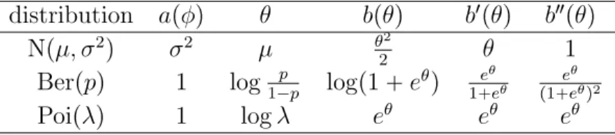
which includes many common exponential family distributions, such as Bernoulli, Poisson and Normal with known variance (see Table 2.1).

Table 2.1: Three commonly used distributions in the exponential family. distribution apφq θ bpθq b1pθq b2pθq

Npµ, σ2q σ2 µ θ₂2 θ 1

Berppq 1 log₁p_p logp1 eθq ₁eθ_eθ

eθ

p1 eθ_q2

Poipλq 1 logλ eθ _eθ _eθ

Rather than using all predictors, we may wish to consider models based on a subset of V. Suppose X0 is the set of predictors common all models and VM is the subset of V in model M, then we can write model in (2.4) as

ηM X0α0,M VMβM, (2.5)

where typically, X0 1n.

In normal linear models, the most common variant of the g-prior is

βM |σN 0, g I_n1pβMq

,

where InpβMq XTMXM{σ2. The precision matrix (i.e., inverse covariance) of

this g-prior equals the inverse of the hyper parameter g multiplied by the expected information matrix based on all n observations, which is the same as the observed information. Extensions are more complicated for non-Gaussian distributions in the exponential family, because their information matrices depend on the unknown coefficient parameters. Bov´e and Held (2011) evaluate the expected information matrix at the prior mode zero, while Hansen and Yu (2003) at the MLE estimates

ˆ

βM. Wang and George (2007) also evaluate the information at the MLE, but use the

observed information matrix instead. Gupta and Ibrahim (2009) avoid this choice by keeping the unknown parameterβM in the prior precision matrix, which leads to

(25)

2.2.2 “Centering” the Predictors

Bov´e and Held (2011) point out that majority of the current variants of g-priors for GLMs do not treat the common parameters across models, usually the intercept, differently from the model specific coefficients, so that X0 ø. This means that the intercept or other common parameters are shrunk towards zero along with the coefficients, which may be problematic when the true intercept is large relative to the regression coefficients. In the extreme case, in normal linear models if the true intercept approaches infinity, and g is allowed to adapt to the data, then the null model is selected. Hence it is desirable to assume the common parameters and the model specific parameters are independent a priori. Motivated by the projection procedure (1.4) in normal linear models, which ensures orthogonality between the common variables X0 and the model specific predictors XM, we propose a “center-ing” procedure for likelihood densities in the exponential family, to ensure that the expected Fisher information is block diagonal.

Proposition 1. Under any modelM, we propose the following “centering” procedure

to transform its model specific predictors VM to XM,

XM InPˆX0 VM, (2.6) ˆ PX0 X0 X T 0InpηˆMqX0 1 XT₀InpηˆMq, (2.7) ηM X0αM XMβM, (2.8)

where InpηˆMq is the expected information matrix of ηM pη1,M, . . . , ηn,MqT

evalu-ated at its MLE based on all n observations. After this reparameterization,

XT₀InpηˆMqXM0, (2.9)

(26)

at the MLE In ˆ αM,βˆM InpαˆMq 0T_n 0n InpβˆMq (2.10)

is block diagonal. Note that PˆX0 is an orthogonal projection on the column spaceX0

with inner product xx,yy xT_I

npηˆMqy.

Proof. Since the linear combination ηM does not change under the translation

op-erator, due to the functional invariance of MLEs, ˆηM remains the same after (2.6).

We can simply verify that the off-diagonal block of the information matrix equals zero (2.9).

In most GLM variable selection problems, the only common predictor is the intercept X0 1n. Then after the “centering” step (2.6), the j-th predictor

Xj Vj 1nv˜j,M, (2.11)

where ˜vj,M is a weighted average of elements of the vector Vj and the weights

de-pending on the information matrix InpηˆMq. In particularly, under normal linear

models, these weights are equal and thus ˜vj,M becomes the column-wise average.

Except for normal distributions, the “centering” procedure (2.6) is model specific due to its dependence on model specific MLEs in the inner productInpηˆMq. Due to

the asymptotic consistency of the MLE, we now treat the parameter αM as a

com-mon parameter across models, and αM and βM are treated differently by having

independent prior distributions, i.e.,

ppαM,βMq ppαMqppβMq. (2.12)

The “centering” step also simplifies the calculation of the marginal likelihood. Under most of the distributions in the GLM family (except for normal distribution), the marginal likelihood does not have a closed form. To calculate the marginal like-lihood, we apply a Laplace approximation (Tierney and Kadane, 1986) that utilizes

(27)

a second order Taylor expansion around the MLEpαˆM,βˆMq. ppY |Mq » fMpY|αM,βMqppαMqppβMq dpαM,βMq (2.13) fMpY |αˆM,βˆMq » e12pαMαMˆ qTInpαMˆ qpαMαMˆ q ppα_Mq dα_M (2.14) » e12pβMβMˆ q T_I npβMˆ qpβMβMˆ q _pp_β Mq dβM Opn1q. (2.15)

According to Kass et al. (1990), this Laplace approximation is precise to the order of

Opn1q. The “centering” step combined with independent prior distributions forαM

andβM allows us to approximate the marginal likelihood by integrating outαMand

βM separately. Next, we will describe the g-prior for GLMs that we adopt, which

leads to closed form marginal likelihood under the Laplace approximation (2.14), as well as extensions to mixtures of g-priors.

2.2.3 Theg-prior for GLMs

In normal linear models, Zellner’s g-prior for (1.6) (1.7), assigns the model specific coefficient βM a multivariate normal prior distribution centered at zero, and the

inverse of its prior covariance is proportional to the information matrix InpβMq XT

MXM{σ2. In GLMs, the expected information matrix becomes

InpβMq XMT InpηMq XM

XT_M r∆pηMq InpθMq∆pηMqs XM,

where ∆pηq denotes the diagonal matrix whose i-th element is dθi

dηi evaluated at the

i-th linear predictor ηi,M αM xTi,MβM, and InpθMq denotes the expected

in-formation matrix of θM based on all n data points. Under canonical links, ∆pηMq

becomes the identity matrix, and hence InpηMq becomes the diagonal matrix with

elements b2pηi,Mq.

In GLMs, after “centering” the design matrix to XM, we propose the following definition of the g-prior under modelM. We letβ have a normal prior with mean

(28)

0 and covariance being proportional to inverse of the expected information matrix, and let the interceptαM have an independent normal prior:

βM |g,MNpM

0, gInpβˆMq1 , (2.16)

ppαM |Mq Np0, ncq, (2.17)

where g is a positive parameter, InpβˆMq is the expected information matrix based

on all the data and evaluated at the MLE pαˆM,βˆMq in the form of ˆηM, and c is

a non-negative constant. In the literature, such data dependent priors have been proposed, for example, Kass and Wasserman (1995), Hansen and Yu (2003) and Wang and George (2007). Notice as when c 8, (2.17) degenerates to the flat prior ppαMq 9 1. Although in linear model, the flat prior on the intercept is a

prevalent choice in almost all existing variants of g-priors that treat the intercept and coefficient separately, we will show in Section 2.4.2 that this may be problematic for other GLM functions.

2.2.4 Laplace Approximate of the Bayes Factor

As discussed in (2.14), we utilize the Laplace approximation to calculate the marginal likelihood for modelM. The normal densities ofαM andβMfrom the likelihood can

be combined with the independent normal prior densities onαMandβM(2.16) (2.17)

respectively. Hence we obtain the approximate marginal likelihood in analytical form,

ppY |g,Mq fM Y|αˆM,βˆM r1 InpαˆMqncs 1 2 _e InpαˆMqαˆ2_M 2pInpαˆMqnc 1q _(2.18) p1 gqpM2 e Q_M 2p1 gq _Op_n1q_, _(2.19) where QM ˆ βMT XTM InpηˆMq XMβˆM (2.20) is the analogue of the regression sum of squares in the linear model,pMis the number

(29)

intercept. Note that for the null modelMø wherepMø 0, we can let QMø 0 and

then (2.18) remains to hold. When comparing two models M2 to M1, the Bayes factor under g-prior can be approximated as the ratio of their marginal likelihoods, which can be rewritten as

BFM2:M1 ΛM2:M1 ΩM2:M1 Opn

1_q_, _(2.21)

which is decomposed to the product of

ΛM2:M1 fM2pY|αˆM2,βˆM2q fM1pY|αˆM1,βˆM1q 1 InpαˆM2qnc 1 InpαˆM1qnc 1 2 e 1 2 Inpαˆ_M 2qαˆ 2 M₂ InpαˆM₂qnc 1 Inpαˆ_M 1qαˆ 2 M₁ InpαˆM₁qnc 1 (2.22) and ΩM2:M1 p1 gq p_M 2 2 exp ! QM₂ 2p1 gq ) p1 gq pM₁ 2 exp ! QM₁ 2p1 gq ). (2.23)

The first term ΛM2:M1 consists of the maximized likelihood ratio and the penalties

contributed by the intercept. The second term ΩM2:M1 comes from the generalized

g-prior on the coefficients. In particular, the choice ofg effects the Bayes factor only through ΩM2:M1.

Note that if c 8, i.e., the prior distribution on αM is the flat prior, then the

approximate Bayes factor and its corresponding ΛM2:M1 become

ppY|g,Mq fM Y |αˆM,βˆM p2πq 1 2 rI npαˆMqs 1 2 p₁ _gq p_M 2 e QM 2p1 gq _Op_n1q_, (2.24) where Λc_M8₂_:_M₁ fM2pY|αˆM2,βˆM2q rInpαˆM2qs 1 2 fM1pY|αˆM1,βˆM1q rInpαˆM1qs 1 2 . (2.25)

(30)

2.2.5 Approximate Conditional Posterior Distributions

For any given model M, here we consider the conditional posterior distributions of

αM and βM under our g-prior (2.16), (2.17) for GLMs. For notation simplification,

when there is no ambiguity, we omit the subscript M. Except for the normal dis-tribution, other likelihood densities in GLMs (2.1) are not conjugate with normal prior on αM and βM. Fortunately, according to the standard Bayesian asymptotic

theory (see Bernardo and Smith (2000), p287), asn increases, the conditional poste-rior densities based on observed data tY,Vu tpY1,v1q, . . . ,pYn,vnqu converges to

normal densities, αM |Y,M d ÝÑN InpαˆMq InpαˆMq _nc1 ˆ αM, 1 InpαˆMq _nc1 , (2.26) βM |Y, g,M d ÝÑN g 1 g ˆ βM, g 1 g InpβˆMq 1 , (2.27)

hence we can use these normal distributions as approximates to the conditional posterior distributions. Note that when flat prior is assigned to αM, i.e., c 8, its

approximate conditional posterior is

αM |Y,M

d

ÝÑN ˆαM, rInpαˆMqs1

.

Similar to the posterior distribution under Zellner’s g-prior in the normal lin-ear models, the approximate conditional posterior mean of βM is shrunk from the

MLE ˆβM towards 0. We donate the ratio z g{p1 gq between the posterior

mean _EpβM | Y, g,Mq and the MLE ˆβM as the shrinkage factor. Assume that

the expected information InpβˆMq based on all data is proportional to n, then the

approximate posterior covariance ofβM is proportional with 1{n. Therefor, the

con-ditional posterior ppβM | Y, g,Mq becomes more concentrated around its mean as

(31)

2.2.6 Inconsistency of the g-prior

For our model selection problem, suppose among all the 2p different models, there exists a true modelMT that generates the data. Under the true modelMT, the MLE

ˆ

βMT converges to the true parameter β

MT, while the conditional posterior mean

ErβMT |Y, g,Msbecomes more concentrated around ˆβMT g{p1 gq. Therefore, with

any fixed value of g, the posterior mean estimate of βMT is biased asymptotically.

In addition to the inconsistency in parameter estimation, g-priors with fixed g

also exhibits inconsistency in model selection. In normal linear models, Liang et al. (2008) points out the selection inconsistency of g-prior with fixed g. They also suggest that some fully Bayes methods that assigns prior distributions on g, such as the Zellner-Siow prior (Zellner and Siow, 1980), the Hyper-g prior and the Hyper-g{n

prior (Liang et al., 2008) can partially or completely resolve this inconsistency. We find that in GLMs, this inconsistency also exists with fixed g. The following counter example shows that in normal linear model with fixed variance, when comparing two nested models, if the smaller model is the true model MT, the Bayes factor for MT

compared toM under g-prior does not go to8 asymptotically.

Remark 1. Under normal linear model with known variance σ2 ₁_{, for any fixed}

value ofg and any model MMT, as the sample sizen increases, the Bayes factor

under the g-prior (2.16), (2.17)

BFMT:MOp1q,

which implies the selection consistency does not hold for g-prior with fixed g.

(32)

2.3 The Confluent Hypergeometric Prior on

g

We propose a hierarchical prior distribution ong to resolve the inconsistency. Based on the g-prior (2.16), (2.17), we assign a hyper prior distribution,

ppg |a, b, sq ga21p1 gq a b 2 exp s 2 g 1 g Bpa₂,b₂q 1F1pa₂,a b₂ ,s₂q , (2.28)

where parameters a ¡ 0, b ¡ 0, s ¥ 0, and 1F1 is the confluent hypergeometric function (Abramowitz and Stegun, 1970). (See Appendix A.1 for definition of the1F1 function). Gordy (1998a) proposes the Confluent Hypergeometric (CH) distribution, which can be considered as a generalization of Beta distribution and has the following density function

pCHpz |a, b, sq z

a1p₁_zqb1_expp_szq

Bpa, bq 1F1pa, a b,sq

, 0¤z ¤1, (2.29) where parameters a ¡ 0, b ¡ 0 and s P _R. When s 0, the CHpa, b, sq distribution degenerates to Betapa, bq distribution. When transforming g to the shrinkage factor

z, the prior distribution (2.28) becomes a CH distribution on z, i.e.,

z g 1 g CH a 2, b 2, s 2 , (2.30)

which guarantees that the prior distribution (2.28) is well-defined. It is also a con-jugate prior, in that the conditional posterior distribution ofz also has a CH distri-bution, z |Y,MCH a 2, b pM 2 , s QM 2 , (2.31)

wherepM is the model size ofM, andQM βˆMT XTMInpηˆMqXMβˆM is the analogue

of RSS in GLMs. We denote the hierarchical g-prior (2.16), (2.17) and (2.28) as the CH-g prior.

(33)

2.3.1 Tail Behavior of the CH-g Prior

Heavy-tailed prior distributions on βM are desirable in model selection since they

are robust to large coefficients in terms of not over-shrinking them. Most state of the art prior distributions ong yield the prior densities of ppβM |Mqwith multivariate

Student tails, for example, Zellner and Siow (1980), Liang et al. (2008), Maruyama and George (2011) and Bayarri et al. (2012). The following proposition shows that under the CH-g prior, the prior distribution on βM also behaves as a multivariate

Student distribution in the tails.

Proposition 2. Under the CH-g prior (2.16), (2.17) and (2.28), the marginal prior

distribution under model M

ppβM |Mq

»

ppβM |g,Mqppgqdg

has tails behave as multivariate Student distribution with degrees of freedom b and

scale matrix InpβˆMq 1 , i.e., lim }βM}Ñ8ppβM |Mq9 }βM} 2 In b pM 2 _, _(2.32) where }βM} pβMT βMq 1 2 and }β_M}_I n βT MInpβˆMqβM 1 2 .

Proof: see Appendix A.2.2.

The choice of the hyper parameter b alone determines the tail behavior of the marginal prior ppβM|Mq. In particular,b 1 corresponds to Cauchy tails.

2.3.2 Approximate Bayes Factor under the CH-g Prior

Similar to theg-prior for GLMs, the CH-g prior also yields closed-form marginal like-lihood under Laplace approximations. Denote u1z, then the prior distribution

(34)

onz (2.30) is equivalent to u 1 1 g CH b 2, a 2, s 2 . (2.33)

Hence we can integrate g (in the form of u) out from (2.18) and obtain the approxi-mate marginal likelihood under the CH-g prior for model M

ppY |Mq »1 0 ppY|u,Mqppuqdu fM Y|αˆM,βˆM r1 InpαˆMqncs 1 2 _e InpαˆMqαˆ2_M 2pInpαˆ_Mqnc 1q B b pM 2 , a 2 1F1 b p₂M,a b p₂ M,s Q₂M B b₂,a₂ 1F1 b₂,a b₂ ,₂s Opn1q.

Therefore, the Bayes factor comparing M2 to M1 under the CH-g prior can be approximated as BFM2:M1 ΛM2:M1 Ω CH M2:M1 Opn 1_q , (2.34)

where ΛM2:M1 remains the same as in (2.22) and

ΩCH_M₂_:_M₁ B _{b p} M₂ 2 , a 2 1F1 _{b p} M₂ 2 , a b pM₂ 2 , s QM₂ 2 B b pM₁ 2 , a 2 1F1 b pM₁ 2 , a b pM₁ 2 , s QM₁ 2 . (2.35)

We can further let hyper parametersa, b, sto be model specific, then the normalizing constants from the prior in (2.35) can not be canceled, i.e.,

ΩCH_M₂_:_M₁ B _b M₂ pM₂ 2 , aM₂ 2 1F1 _b M₂ pM₂ 2 , aM₂ bM₂ pM₂ 2 , sM₂ QM₂ 2 B bM₁ pM₁ 2 , aM₁ 2 1F1 bM₁ pM₁ 2 , aM₁ bM₁ pM₁ 2 , sM₁ QM₁ 2 (2.36) B _b M₁ 2 , aM₁ 2 1F1 _b M₁ 2 , aM₁ bM₁ 2 , sM₁ 2 B bM₂ 2 , aM₂ 2 1F1 bM₂ 2 , aM₂ bM₂ 2 , sM₂ 2 . (2.37)

(35)

2.3.3 Connection with the Literature

Note that the density function of the Confluent Hypergeometric distribution (2.29) is proportional to the densities of both Beta distribution and truncated Gamma distribution, which implies that our CH ₂b,a₂,₂s prior on u1{p1 gq encompasses some of the exsiting prior distributions on the hyper parameter g.

In normal linear models, to achieve marginal likelihoods in closed forms, prior dis-tributions onuoriginating from the Beta distribution are conventional. For example, Liang et al. (2008) introduces the Hyper-g prior,

1

1 g Beta

_a

h

2 1,1 , (2.38)

where 2 ah ¤ 4. When ah 4, the Hyper-g prior is equal to the uniform prior.

The recommended value of the hyper parameterah 3 corresponds to a proper prior

which puts more mass of 1{p1 gq near 0. The choice ah 2 corresponds to both

the reference prior and the Jeffrey’s prior, which is improper. While it yields proper posterior distributions, because g does not appear in the model with just X0, Bayes factors are ill-determined due to the arbitrariness of the constants of proportionality. The Hyper-g prior (2.38) can be viewed as a special case of our CH-g prior, with

a2, bah2 and s0.

The marginal likelihoods under the Hyper-g prior in normal linear models have closed forms that contain the Hypergeometric 2F1 function. To further simplify the marginal likelihood, Maruyama and George (2011) proposes the Beta prior distribu-tion ong, 1 1 g Beta 1 4, npM 2 3 4 , (2.39)

which eliminates the need to evaluate the2F1 function in the marginal likelihood. An additional benefit is the fact that the second parameter being proportional with n

(36)

yields an implicit Opnqchoice on g. According to the authors, g Opnq in the prior is desirable since it prevents the prior variance on βM from decreasing to zero and

prevents the likelihood from being dominated by g asymptotically. The Beta prior (2.39) is also a special case of the CH-g prior, with anpM1.5 and b0.5.

In GLMs, when the precision apφqis fixed, the likelihood under Laplace approxi-mate usually contains an exponential term ofu, for example, (2.18). Hence conjugate prior densities of u should contain some form of Gamma distribution density. For example, Wang and George (2007) proposes the truncated Gamma prior on u,

1

1 g Gammap0,1qpat, btq, (2.40)

where the domain is restricted to the interval p0,1q, andat¡0, bt¡0. The authors

recommend to use a uniform prior ong, which can be achieved by settingat1, bt

0. The CH-g prior also encompasses (2.40), with a2, b 2at and s2bt.

Although our CH-g prior encompasses the above prior distributions on g, it does not include the Hyper-g{n prior (Liang et al., 2008) and the Robust prior (Bayarri et al., 2012). Since the Hyper-g prior cannot yield consistency for model selection when the null model is true, Liang et al. (2008) modify it to the Hyper-g{n prior,

ppgq ah2 2n 1 1 g{n ah{2 , (2.41) where 2 ah ¤4.

Under the Robust prior (Bayarri et al., 2012), after transforming the parameter

g tou1{p1 gq, we find that its prior density becomes

prpuq arrρrpbr nqsar

uar1

r1 pbr1qus

ar 1 1t0 u _ρr_p_{br n}1_{q p}₁_br_qu, (2.42)

wherear ¡0, br ¡0 andρr ¥ _b_rbr_n. In normal linear models, the Robust prior yields

(37)

the various criteria for model selection priors proposed in Bayarri et al. (2012), the recommended values of the hyper parameters in the Robust prior arear 0.5, br 1

and ρr 1{p1 pMq. Both the Hyper-g prior and the Hyper-g{n prior are special

cases of the Robust prior. More specifically, (2.42) with ar ah{21, br 1, ρr

1{p1 nq becomes the Hyper-g prior and (2.42) with ar ah{21, br n, ρr 0.5

corresponds to the Hyper-g{n prior. The CH-g prior cannot be obtained as a special case of the Robust prior.

2.3.4 A More General Class of Prior Distributions on g

Both the Robust prior and the CH-g prior are special cases of a more general class of distributions, the Compound Confluent Hypergeometric (CCH) distribution (Gordy, 1998b). The CCH distribution has 6 parameters and can be considered as a gener-alized version of the Confluent Hypergeometric distribution. Suppose variable uhas CCH distribution, then its density function is

pCCHpu|t, q, r, s, v, θq (2.43) vtexpps{vq Bpp, qq Φ1pq, r, t q, s{v,1θq ut1p1vuqq1esu rθ p1θqvusr 1t0 u 1vu, (2.44) where t¡0, q ¡0, rP _R, sP_R,0¤v ¤1, θ¡0, and Φ1pα, β, γ, x, yq 8 ¸ m0 8 ¸ n0 pαqm npβqn pγqm nm!n! xmyn

is the confluent hypergeometric function of two variables (Gordy, 1998b). We can extend the possible domain of the CCH distribution to p0,1{vq with v ¡1, so that the upper bound of u can be strictly below 1. The extended CCH distribution as a prior distribution on u1{p1 gq unifies a broader variety of prior distributions including both the Robust prior and the CH-g prior. The Robust prior is equal to

uCCH ar,1, ar 1,0, ρrpbr nq p1brq,1 1br ρ pb nq

(38)

and the CH-g prior is equal to uCCH b 2, a 2,0, s 2,1,1 .

In GLMs, under the extended CCH prior on u, the approximate marginal likeli-hood also has a closed form.

ppY |Mq »1 0 ppY |u,Mqppuqdu fM Y|αˆM,βˆM r1 InpαˆMqncs 1 2 e Inpαˆ_Mqαˆ2_M 2pInpαˆ_Mqnc 1q B 2t pM 2 , q vpM2 e QM 2v Φ₁ q, r,2t 2q pM 2 , 2s QM 2v ,1θ Bpt, qq Φ1 q, r, t q,_vs,1θ Opn 1_q_.

Under the Robust prior with b 1, the Φ1 function in ppY | Mq degenerates to a truncated Gamma function, which is easier to compute; that is

ppY|Mq fM Y|αˆM,βˆM r1 InpαˆMqncs 1 2 _e InpαˆMqαˆ2_M 2pInpαˆMqnc 1q_a rrρrp1 nqs ar QM 2 p_M 2 ar" Γ _p M 2 ar Γ pM 2 ar, QM 2ρrp1 nq * Opn1q,

where Γpaq is the Gamma function and Γpa, sq ³_s8ta1etdt is the incomplete Gamma function.

2.4 Model Selection Consistency

In this section, we will focus on the asymptotic model selection performance of the CH-g prior for GLMs. In addition, we also study its behavior in a special but not rare case, where the sample size is small and there exists a model that fits the data perfectly.

(39)

2.4.1 Asymptotic Consistency for Model Selection

When studying the asymptotic properties, we believe it is reasonable to assume that the unit expected information matrices are non-singular.

Assumption 1. We here assume a mild condition on the predictors r1n,Xs in the

full model. For any n-dim vector η in the space spanning by the predictorsCp1n,Xq,

i.e.,η r1n,Xsw, where wis ap1 pq-dim vector of weights, there exists a positive

definite matrix Σw such that

lim

nÑ8

r1n,XsT Inpηq r1n,Xs

n ÝÑΣw (2.45)

In normal linear model, this assumption implies that XTX{n converges to a pos-itive definite matrix Σ0, which is a conventional assumption in the model selection literature. Furthermore, if we treat the rows of the full design matrix Xas indepen-dent random samples from p-dimensional multivariate distributions which have the same mean and bounded covariance, then (2.45) holds according to the Law of Large Numbers.

Remark 2. Before studying the asymptotic consistency of the CH-g prior, we want

to point out that most asymptotic results which require i.i.d. samples as their

con-ditions also hold under GLMs. Although in GLMs, observations Y1, . . . , Yn are

con-ditionally independently but not identically distributed, we can assume that jointly

pY1,x1q, . . . ,pYn,xnq are i.i.d random samples. Thus as long as the marginal

distri-bution of xdoes not depend on the GLM parameters, the log-likelihood and the score

functions do not depend on the marginal distribution of x. Hence the asymptotic

results related to the MLE and likelihood ratio test also hold here. This underlying assumption is adopted by van der Vaart (2000) (Ch5) when applying MLE consis-tency in regression examples.

(40)

According to Self and Mauritsen (1988), within the framework of GLM, for every modelM, the MLE of its parameterspαˆM,βˆMqconverges topαM,βM qin probability

as n increases, where limit pα_M,β_M q are the maximizers of the limit of the log-likelihood,

pα_M,β_M q argmax_p_α,_β_q lim

nÑ8

1

nlogfMpYn |α,βq.

In particular, in the true modelMT,pαMT,β

MTqare true parameters which generate

the data.

We consider the same model selection consistency criteria discussed by Fernandez et al. (2001), Liang et al. (2008) and Bayarri et al. (2012).

Definition 1 (consistency for model selection). Suppose the true model that

gener-ates the data is among the 2p _{potential models, and we denote it as} _M

T. We say

that the Bayes rule under the 0-1 loss is consistent for model selection if

plim_n_Ñ8 ppMT |Yq 1 (2.46)

This means that for any model M MT, plimn ppM | Yq 0. Hence a

sufficient condition for model selection consistency is that

plim_n_Ñ8 BFMT:M 8 (2.47)

for any M MT, assuming fixed prior odds. The counter example in Remark 1

shows that for any fixed g, the consistency for model selection do not hold under the fixedg-prior for GLMs, thus we focus on results under the CH-g prior. According to our previous decompositions of the Bayes factors (2.34), it is sufficient to examine the asymptotic properties of ΛMT:M and Ω

CH

MT:M.

We will show in the following lemma that the first term ΛMT:M(2.22) of the Bayes

factor is dominated by the maximized likelihood ratio asymptotically. According to Self et al. (1992), under the alternative model, the log likelihood ratio between MT

(41)

Lemma 1. As the sample size n increases, the asymptotic property of ΛMT:M fMTpY|αˆMT,βˆMTq fMpY|αˆM,βˆMq 1 InpαˆMTqnc 1 InpαˆMqnc 1 2 e 1 2 Inpαˆ_M Tqαˆ 2 M_T InpαˆM_Tqnc 1 Inpαˆ_Mqαˆ2_M InpαˆMqnc 1 is that 1) if MT M, then ΛMT:M Op1q; 2) if MT M, then ΛMT:M Ope

cnq_{, where} _c _{is a positive constant.}

In addition, under the flat prior ppαMq91, these properties also hold for

Λc_M8 T:M fMTpY|αˆMT,βˆMTq fMpY|αˆM,βˆMq InpαˆMTq InpαˆMq 1 2

Proof: see Appendix A.2.3.

The first term ΛMT:M in the Bayes factors can be considered as a measure of

goodness of fit. If the space spanned by the predictors of M does not contain all predictors in the true model MT, M cannot predict as well as MT. Therefore, the

term ΛMT:M overwhelmingly favors MT by increasing at an exponential rate of n.

On the other hand, when the design space of Mcontains all predictors in MT, M

has the same ability in explaining the response asMT. Therefore, ΛMT:Malone does

not favor selecting MT against a redundant modelM. In this case, the second term

in the Bayes factors, (2.23) or (2.35), plays a more important role of placing more penalty on the redundant model. In the case of fixed g, the termp1 gqppMpM_Tq{2

in ΩMT:M penalizes M for the extra dimensions. However, the counter example in

Remark 1 illustrates that with fixedg, the penalty being imposed on the redundant model is not strong enough asymptotically. Next, we will focus on the CH-g prior by exploring the asymptotic properties of ΩCH , which yields a stronger penalty on

(42)

the model size. We first study the asymptotic behavior of the analogue of regression sum of squares (RSS) for GLMs, QMT and QM in the following lemma.

Lemma 2. Let β_M denote the limit of the MLE βˆM. The asymptotic properties of

QM ˆ β_MT XT_M InpηˆMq XMβˆM

under the true model MT and under any other model M are

1) If MT Mø, then QMT Opnq; for any other model M, if βM 0, then

QM Opnq, and otherwise, QM Op1q.

2) If MT Mø, then for any model M, QM Op1q; and by the definition of Q

under the null model, QMT Op1q.

Proof: see Appendix A.2.4

Theorem 1. With fixed hyper parameters a, b¡0and s¥0, the CH-g prior (2.28)

is consistent for model selection (2.47), except for MT Mø. In addition, this result

also holds with model specific hyper parameters aM, bM, sM that are independent of

n.

Theorem 1 implies that the CH-g prior is desirable as a model selection prior in most cases. However, it fails to impose a strong enough penalty in the case where the null model is true. To resolve this inconsistency, we allow the hyper parameter

a to increase with n, such that lim

nÑ8

a n a

_{, where}_a _¥₀_. _(2.48)

The following theorem shows that whena ¡0, the selection consistency holds under any MT, including whenMT Mø.

(43)

Theorem 2. With hyper parameters b ¡ 0, s ¥ 0, and limnÑ8a{n a ¡ 0,

the CH-g prior (2.28) is consistent under model selection universally, including the

case where MT Mø. In addition, this result also holds with model specific hyper

parameters aM, bM, sM, where limnÑ8aM{naM ¡0.

2.4.2 Perfect Fitting with Small Sample

We have demonstrated that the CH-gprior for GLMs is consistent for model selection with large n. Now we will explore its selection performance with small samples, in the case of perfect fitting.

In linear regression, Liang et al. (2008) points out that under the Zellner’s g-prior with any fixed value ofg, there exists the following information paradox. In principle, forn"pM 1, if all the observations fall on a hyperplane (R2 1), the Bayes factor

should support model M overwhelmingly over the null model Mø. However, with any fixed g, the BFM:Mø under the g-prior is bounded. To resolve this information

paradox, the parametergshould be assigned certain hyper prior distributions in fully Bayes approach, or be estimated by empirical Bayes approach.

Bayarri et al. (2012) provide a formal definition of the information consistency for priors in model selection. If there exists a sequence of datasets with the same size

n such that the ratio of maximized likelihoods between M and Mø go to infinity, then their Bayes factors should also go to infinity. The condition of this criteria describes the perfect fitting phenomenon under model M of a diverging likelihood ratio, which is precise in linear regression since the estimate for the normal variance in

Mis equal to zero, i.e., ˆσ2 0. However, this form of perfect fitting is not necessarily true with most GLMs, including logistic regression and Poisson regression. Because the response variable is discrete, the maximum likelihood under M has an upper bound being 1, and no matter how minimal the amount of information the null

(44)

model Mø can reveal, its maximum likelihood is always greater than zero. Hence for discrete distributions in the exponential family, even the GLMs can fit the data perfectly, their likelihood ratios are bounded. For example, in logistic regression, suppose model M fits each binary response perfectly, i.e., ˆµi 1 if Yi 1, and

ˆ

µi 0 if Yi 0; while the estimates of success probability inMø are ˆµi 0.5. The

likelihood ratio

fMpY|αˆM,βˆMq

fMøpY |αˆMøq

4n 8.

We propose to use the fitted variance of all responses being zero to quantify the perfect fitting phenomenon, that is, under model M,

{

VpYiq 0, i1, . . . , n, (2.49)

which is equivalent to fMpY | αˆM,βˆMq 8 in normal distribution. While in

the Bernoulli distribution, although the likelihood function is bounded, our criterion (2.49) precisely describes the perfect fitting phenomenon. When the fitted values of the expectation of every binary response _EzpYiq equals to 0 or 1, the fitted values of

the variances are zero.

Another interesting difference we find between normal linear regression and GLMs is whether to favor M over the null if perfect fitting occurs, but the sample size is relatively small. In normal linear regression, as Liang et al. (2008) and Bayarri et al. (2012) suggest, perfect fitting with any n ¥pM 2 is strong evidence to favor M.

However with discrete responses, especially binary ones, perfect fitting is likely to occur by chance when n is just slightly larger than pM 1. In this case, the Bayes

factor should not overwhelmingly supportMoverMø, unlessnis large enough. This problem is worth noticing because it is not rare in real world applications where p

(45)

expected information of the i-th linear combination Inpηîq eηî p1 eηîq2 or φpηîq2 p1ΦpηîqqΦpηîq

converges to zero as ˆηi 8, whereφpq,Φpqare pdf and cdf of the standard normal

distribution. If perfect fitting occurs under modelM, thenInpαMq 0 andQM 0.

According to the Laplace approximation of marginal likelihoods, Λc_M8_:_M_ø 8(2.25). Since both ΩM:Mø (2.23) and Ω

CH

M:Mø (2.35) are bounded, BFM:Mø diverges under

both g-prior and CH-g prior. In contrast, under the normal prior on the intercept, because ΛM:Mø is bounded, this problem is resolved. In Section 2.2.3, we recommend

using a proper prior (2.17) on the intercept instead of the commonly used improper flat prior, to avoid inconsistency with perfect fitting with small n, where the Bayes factor overwhelmingly supports the larger model.

On the other hand, if perfect fitting occurs under modelMwith sufficiently large samples, it is reasonable to let the BFM:Mø go to infinity. We set the prior variance

ofαMproportional to n, so that the normal prior converges to flat prior asnincrease

which indicates model M is overwhelmingly favored if it can fit a large sample of responses perfectly and the estimate of αM is consistent.

2.5 BMA Estimation Consistency

2.5.1 Asymptotic Posterior Estimates

In each model MMø, the conditional posterior mean

ErβM|Y, g,Ms

g

1 g

ˆ

βM

does not converge to the limit of the MLE asymptotically with any fixedg. In a fully Bayes approach, convergence of the posterior distribution of the shrinkage factor

(46)

zβˆM being consistent. Before examining the parameter estimation consistency of

the coefficients, we first study the asymptotic behavior of the conditional posterior

ppz | Y,Mq. in the following propositions. Since these results are studied under each model M, they remain true if we allow the hyper parametersaM, bM, sM to be

model specific. For notation simplicity, we omit their subscriptM here.

Proposition 3. For the CH-g prior with hyper parameters a ¡ 0, b ¡ 0, s ¥ 0,

if the MLE of its coefficient converges to a non-zero vector βˆM Ñ βM 0, then

the conditional posterior distribution of z g{p1 gq under any model M Mø,

converges to 1 in probability

plim_n_Ñ8 ppz |Y,Mq δ1pzq (2.50)

In particular, if the true model is not null MT Mø, (2.50) holds underMT.

Proposition 4. For the CH-g prior with hyper parameters b ¡ 0, s ¥ 0, and

limnÑ8a{n a ¡ 0, for any true model MT including MT Mø, the

condi-tional posterior distribution of the shrinkage factor z g{p1 gq under any model

MMø converges to 1 in probability, i.e., (2.50).

2.5.2 Parameter Estimation under BMA

Bayesian model averaging (BMA) estimates are widely used to incorporate model uncertainty. We denote the variable β as the p dimensional vector of coefficients corresponding to all the potential predictors. In this section, we slightly abuse the notations βM by redefining that as a p-dimensional vectors filled with zeros for

(47)

distribution of β under BMA is

ppβ |Yq ¸ M

ppM|Yq ppβM |Y,Mq, (2.51)

where the marginal posterior distribution under model Mcan be calculated as

ppβM |Y,Mq » ppβM |Y, g,Mqp g 1 g |Y,M d g 1 g. (2.52)

To study the parameter estimation performance of the BMA estimates asymptoti-cally, we propose the following estimation consistency.

Definition 2 (consistency for parameter estimation). The parameter estimation

un-der BMA is consistent if the posterior of β converges to the true parameter in

prob-ability as n increases, i.e.

plim_n_Ñ8 ppβ |Yq δ_β

M_Tpβq. (2.53)

Under BMA, the posterior distributionppβ|Yqcan be decomposed as a weighted average of the posterior under MT and under other models,

ppβ|Yq ppMT |Yq ppβMT |Y,MTq

¸

MMT

ppM|YqppβM |Y,Mq, (2.54)

To verify the BMA estimation consistency under the CH-g prior, we can use the results on model selection consistency in Section 2.4.1. When the selection consis-tency holds, i.e., ppMT | Yq converges to 1, the second term in (2.54) diminishes

in the limit. Hence in this case, we just need to focus on the posterior distribution of βMT. On the other hand, when the selection consistency does not hold, which

only occurs where MT Mø and aOp1q, we need to examine the limit distribu-tion of ppβM | Y,Mq under every M. Fortunately, in this case the true parameter

β_M

T 0. Although shrinkage always exists, the limit of ppβM | Y,Mq remains 0.

(48)

Theorem 3. With hyper parameters b ¡ 0, s ¥ 0, and limnÑ8a{n a ¥ 0, the

CH-g prior (2.28) is consistent for parameter estimation of the coefficient under

BMA (2.53). In addition, this result also holds with model specific hyper parameters

aM, bM, sM.

2.5.3 BMA Estimation for a New Case

In addition to the current datatY,Vu, if we have a new case and know the values of its exploratory variablesvP_Rp_{, we want to estimate the mean of it response variable}

µ _EpYq under BMA. Under model M, suppose xM vMvM˜ is the vector of new predictors after the “centering” step, where ˜vM is a pM-dim vector consists of

˜

vj,M as in (2.11). The BMA estimate for the mean of the new response is

where the conditional posteriors of αM and βM are approximated by (2.26) and

(2.52). Similarly to the prediction consistency criterion introduced in Liang et al. (2008), we define the estimation consistency under BMA for a new case for GLMs.

Definition 3. We say that the BMA estimation µfor a new case v is consistent if

plim_n µb1pα_M T x T MTβ MTq, (2.55)

where MT is the true model, xMT is the sub-vector of the “centered” new exploratory

variable corresponding toMT, and αMT,β

(49)

We again decompose the BMA estimate µinto the sum of two terms µ ppMT |YqE b1pαMT x T MTβMT |Y,MTq ¸ MMT ppM|Yq _Eb1pαM xTMβM |Y,Mq ,

In the following theorem, we find that the BMA estimation consistency for a new case holds under the CH-g prior.

Theorem 4. With hyper parameters b ¡ 0, s ¥ 0, and limnÑ8a{n a ¥ 0,

the BMA estimation for a new case under the CH-g prior (2.28) is consistent. In

addition, this result also holds with model specific hyper parameters aM, bM, sM.

2.6 Simulation and Real Examples

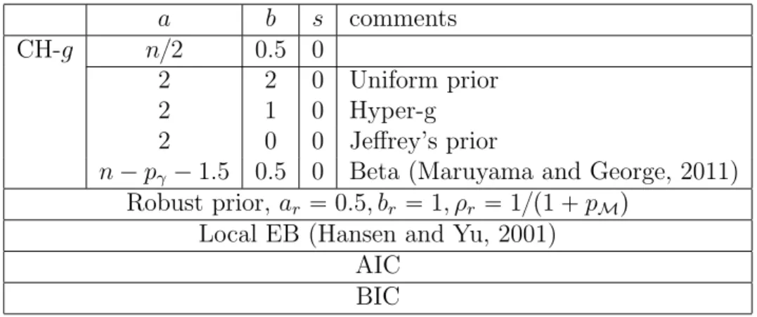
In Section 2.3.3, we have established theoretical connections between our CH-g prior and some of the commonly used prior distributions on the hyper parameter g pro-posed for theg-prior, such as the uniform prior (Wang and George, 2007), the Hyper-g prior (LianHyper-g et al., 2008), the Beta prior (Maruyama and GeorHyper-ge, 2011) and the Robust prior (Bayarri et al., 2012). In this section, using both simulation studies and a real example, we will compare model selection and parameter estimation per-formance across these hyperpriors of g under our extension of the g-prior for GLMs (2.16), (2.17). In addition to the above-mentioned approaches, we also examine the Jeffrey’s prior on g (Celeux et al., 2012), the local empirical Bayes (EB) (Hansen and Yu, 2001) method, the Akaike Information Criterion (AIC) and the Bayesian Information Criterion (BIC).

In the local EB approach, the estimate ofgunder each modelMis the maximizer of the marginal likelihood ppY | g,Mq. Under the Laplace approximation (2.18),

(50)

ˆ gEB M is estimated as ˆ gEB_M arg max g ppY |g,Mq max QM pM 1,0 , (2.56)

and the marginal likelihood is obtained by plugging in this estimate pEBpY |Mq

ppY|gˆEB

M,Mq.

Table 2.2: For GLMs: methods to be compared.

a b s comments

CH-g n{2 0.5 0

2 2 0 Uniform prior

2 1 0 Hyper-g

2 0 0 Jeffrey’s prior

npγ1.5 0.5 0 Beta (Maruyama and George, 2011)

Robust prior, ar 0.5, br 1, ρr1{p1 pMq

Local EB (Hansen and Yu, 2001) AIC

BIC

We summarize all these methods to be compared in Table 2.2. For AIC and BIC, we select the model with smallest AIC and BIC; while for all other methods, we select the modelMwith the highest posterior probability, i.e., maximum a posterior (MAP) estimate. In order to take into account the model uncertainty, for both fully Bayes and empirical Bayes methods, we use Bayesian model averaging (BMA) estimates for the parameterβ and exceptions of new responses µ_EpYq. While for AIC and BIC, these estimates are calculated only based on the selected model.

2.6.1 Default Choice of Hyper Parameters ta, b, su in the CH-g Prior

Before exhibiting the examples, we first give our recommendation on values of the hyper parametersa, b, sin the CH-g prior. In general, whenaorsis large, or whenb

(51)

In this case, little shrinkage is imposed on the posterior estimates ofβM. Meanwhile,

this corresponds to high prior concentration of large g, which implies a flat prior on

βM that favors simple models in model selection, and hence is desirable for sparse

problems.

We choose a to be proportional with the sample size n, to allow the CH-g prior to be consistent for model selection in all circumstances including when MT Mø (see Theorem 2). Some popular methods in linear regression such as Zellner and Siow (1980), the Hyper-g{nprior (Liang et al., 2008), the Beta prior (Maruyama and George, 2011) also recommendg Opnq. Actually under the mild assumption (2.45), the expected information matrix based on alln sample pointsInpβMq Opnq. This

suggests that theg-prior on βM depends implicitly onn, and degenerates to a point

mass at zero in the limit. Hence the choice of g Opnq is essential to avoid having the g-prior to dominate the likelihood. To eliminates the dependency of the prior distribution on specific features of model including the sample size n, Bayarri et al. (2012) proposes the intrinsic consistency of model selection priors, which suggests that as n increase, the prior distribution ppβM | αM,Mq should be proper. In the

context of g-prior (both for normal linear regression and our extension for GLMs), the intrinsic consistency means proper prior distribution on g{n in the limit. With

a Opnq, the CH-g prior yields an implicit g Opnq choice, in the sense that the prior expectation Ep1{gq B a 2 1, b 2 1 1F1 a₂ 1,a b₂ ,s₂ B a₂,b₂ 1F1 a₂,a b₂ ,s₂ ÝÑ b a2 Op1{nq

To choose the default prior rate a a{n, empirical experience indicates no signifi-cant difference in parameter estimation betweena 0.5 and 1. To remain objective and perform well in model selection under both sparse and non-sparse models, we recommend to usea 0.5, i.e. an{2.