EJASA, Electron. J. App. Stat. Anal. http://siba-ese.unisalento.it/index.php/ejasa/index e-ISSN: 2070-5948
DOI: 10.1285/i20705948v7n2p375
Shift point Bayes estimation under Weibull fail-ure model
By Prakash G.
Published: 14 October 2014
This work is copyrighted by Universit`a del Salento, and is licensed un-der aCreative Commons Attribuzione - Non commerciale - Non opere derivate 3.0 Italia License.
For more information see:
DOI: 10.1285/i20705948v7n2p375
Shift point Bayes estimation under
Weibull failure model
Gyan Prakash
∗Department of Community Medicine, S. N. Medical College, Agra, India.
Published: 14 October 2014
The present paper proposes some Bayes estimators for shift point of Weibull failure model under item - failure censoring. The censoring criterion intro-duced first time in present paper for the shift point estimation. Bayes esti-mators obtained here for both known as well as unknown shape parameter cases. A simulation study carried out also for analysis of shift point Bayes estimators and their risks.
Keywords: Shift Point Criterion, Bayes Estimation, Item-failure Censored Data.
1 Introduction
The ’time of failure’ and ’average life’ of a component, measured from some specified time until it fails, is represented by a continuous random variable. Extensively in recent years, one distribution that has been used as a model to deal with such problems for product life is Weibull distribution. The application of the Weibull failure model in life - testing problems and survival analysis has been widely advocated by several authors (Weibull, 1951 ; Berrettoni, 1964). Whittemore and Altschuler (1976) used it as a model in bio-medical applications. It also has been used as model with diverse types of items such as ball bearing (Lieblein and Zelen, 1956), vacuum tube (Kao, 1959), and electrical isolation (Nelson, 1972). Mittnik and Rachev (1993) found that the Weibull distribution might be adequate statistical model for stock returns. Recently, Wahed et al. (2009) consider a new generalization of the Weibull distribution, which incorporates the expo-nentiated Weibull distribution as a special case and its application in a breast cancer.
∗
Corresponding author: [email protected].
c
Universit`a del Salento ISSN: 2070-5948
The probability density function of the considered Weibull distribution is given by
f(x;v, θ) = v
θ x
v−1e−xv
θ ; x >0, v >0, θ >0. (1)
Here the parameter v referred as the shape parameter and θ as the scale parameter of Weibull distribution, respectively. Whenv= 1,the Weibull failure model is Exponential distribution and forv= 2,it is Rayleigh. Further the values lies in the range 3≤v≤4,
the shape of the distribution is close to that of Normal distribution and for a large value of v,say v≥10,is close to that of smallest extreme value distribution. In present arti-cle, we study the properties of the Bayes shift point estimator under all four distributions.
Pandey (1983), Pandey et al. (1989), Chandra and Chaudhari (1990) considered the estimation of the Weibull shape parameter in censored data. Singh and Shukla (2000), Tsionas (2002), Prakash and Singh (2008) and others considered the Weibull distribution in different contexts. Recently, Prakash and Singh (2009) present the estimation of the Weibull shape parameter in failure censored sampling criteria.
The aim of the present article is to discuss about Bayes estimation of the shift point for Weibull failure model under item failure censored data. The shift point criterion discussed in Section 2. The Bayes estimators for shift point are obtained in Section 3 when one parameter is known and in Section 5 when both parameters are considered as random variables. A simulation technique carried out in Section 4 and 6 for the illus-tration of properties of the estimator in terms of posterior risk and Bayes estimate. The sensitivity analysis and conclusion are presented in Section 7 and 8 respectively.
2 The Shift Point
In life testing, fatigue failures and other kinds of destructive test situations, the observa-tions usually occurred in ordered manner such a way that weakest items failed first and then second one and so on. Let us suppose thatnitems are put to test under the model without replacement and the test terminates as soon as firstrth(r ≤n) item fails. This censoring scheme is known as item - failure censoring scheme.
In order to obtain the information on their endurance, manufactured items such as mechanical or electronic components are often put to life tests and life times observed periodically. Physical systems manufacturing the items are often subject to random fluctuations. It may happen that at some point of time, there is a change in the pa-rameter. The objective of study is to find out when and where this change has started occurring. This estimation process is called as the shift point inference problem. The Bayesian model plays an important role in the study of such estimation problem and has been extensively studied by Broemeling and Tsurumi (1987), Jani and Pandya (1999), Ebrahimi and Ghosh (2001). Recently, Pandya and Jadav (2010) presents Bayesian esti-mation of shift point in mixture of left truncated exponential and degenerate distribution.
We are introducing first time the censoring criteria under shift point estimation. For this let us first assume that a sequence of ordered random sample of size n such as
x(1), x(2), ..., x(r−1), x(r), x(r+1), ..., x(n) from the model (1) with parametersθ1 and v.All
nitems are put to test and the test terminates as soon as first rth items fails.
We have a sequence ofr(≤n) ordered random samplex(1), x(2), ..., x(m−1), x(m), x(m+1),
..., x(r) from assumed sample of sizen with survival function Ψ1(t) at any mission time
t(>0),but later it is found that there is a change in the system at some point of time
m(≤r) and it is reflected in the sequence after the itemx(m) by the change in survival
function Ψ2(t).
Thus, first m random observations x(1), x(2), ..., x(m) follow the model (1) with
prob-ability density function
f x(i);v, θ1 = v θ1 xv(i)−1e− xv (i) θ1 ; x(i) >0, v >0, θ1 >0, i= 1,2, ..., m(m≤r, r≤n) (2)
with survival function
Ψ1 x(i) =exp −x v (i) θ1 ! . (3)
First remaining (r−m) componentsx(m+1), x(m+2), ..., x(r)from a sample of sizerfollow
the model (1) with the probability density function
f x(i);v, θ2 = v θ2 xv(i)−1e− xv (i) θ2 ; x(i) >0, v >0, θ2 >0, i=m+ 1, m+ 2, ..., r(m≤r, r≤n) (4)
with survival function
Ψ2 x(i) =exp −x v (i) θ2 ! . (5)
The last remaining group of the random samples x(r+1), x(r+2), ..., x(n) of size (n−r)
follows the Weibull model with parametersv and θ2 and having the probability density
function f x(i);v, θ2 = v θ2 xv(i)−1e− xv (i) θ2 ; x(i) >0, v >0, θ2 >0, i=r+ 1, r+ 2, ..., n(n≥r). (6)
The likelihood function for the shift point under item - failure censoring criterion is defined as L θ1, θ2, m|x(1), x(2), ..., x(r) = m Y i=1 f x(i);v, θ1 ! . r Y i=m+1 f x(i);v, θ2 ! . exp −x v (r) θ2 !n−r! . (7) Solving (7) we have L θ1, θ2, m|x(1), x(2), ..., x(r) = v r θm1 θr2−m r Y i=1 xv(i)−1 ! exp −δ1 θ1 −δ2 θ2 ; (8)
whereδ1=Pmi=1xv(i) andδ2=
Pr i=m+1xv(i)−(n−r)x v (i). Substituting θ1 =θ=θ2 in (8) we have L θ|x(1), x(2), ..., x(r) =v θ r Yr i=1 xv(i)−1 ! exp −δ3 θ ;δ3 =δ1+δ2. (9)
Equation (9) shows the likelihood function under the item - failure censoring criterion without shift point.
Similarly, the likelihood function without shift point under the complete sample case is obtain by substitutingθ1=θ=θ2 and r=n in (8) i.e.
L θ|x(1), x(2), ..., x(n) = v θ n Yn i=1 xv(i)−1 ! exp − n X i=1 xv(i) θ !! . (10)
3 Bayes Estimator for Shift Point (Shape Parameter
Known)
We believe, as stated in Arnold and Press (1983) that from a Bayesian viewpoint, there is clearly no way in which one can say that one prior is better than other. It is more frequently the case that, we select to restrict attention to a given flexible family of priors, and we choose one from that family, which seems to match best with our personal beliefs. One of the best choices of selecting the prior distribution is the conjugate prior. Thus in the present case we considered the inverted Gamma distribution as the natural family of conjugate prior for the parameterθ and defined as
g(θ)∝θ−(α+1)exp −β θ ; α >0, β >0, θ >0. (11)
Under the shift point criterion, the prior information regarding the parameter θ is re -define as gj(θj)∝θ −(αj+1) j exp −βj θj ; αj >0, βj >0, θj >0, j= 1,2. (12)
The prior distribution for the shift point m is considered as discrete uniform over the set (1,2, ..., r−1) and defined as
g3(m) =
1
r−1;r >0. (13)
The joint prior distribution is thus defined as
h(θ1, θ2, m)∝g1(θ1) . g2(θ2) . g3(m).
Hence, the joint posterior density is defined as
Z(θ1, θ2, m) = L θ1, θ2, m|x(1), x(2), ..., x(r) . h(θ1, θ2, m) P m R θ1 R θ2L θ1, θ2, m|x(1), x(2), ..., x(r) . h(θ1, θ2, m)dθ2dθ1 .
After simplification, the joint posterior density is
Z(θ1, θ2, m) = Φθ −(m+α1+1) 1 θ −(r−m+α2+1) 2 exp −ω1 θ1 −ω2 θ2 ; (14) where Φ = (P m∆) −1,∆ = Γ(m+α1) Γ(r−m+α2) ωm+α1 1 ω r−m+α2 2 and ωj =βj+δj ;j= 1,2.
Now, the marginal posterior density for shift pointm is obtain as
Z∗(m) = Φ Z θ1 Z θ2 exp −ω1 θ1 −ω2 θ2 θ1−(m+α1+1)θ2−(r−m+α2+1)dθ2dθ1 ⇒Z∗(m) = Φ ∆. (15)
The Bayes estimator for shift point m under the squared error loss function (SELF) is simply the posterior mean and obtained as
ˆ mS =Ep(m) = Φ X m m∆ ! . (16)
Here, the suffix p indicates the expectation taken under the posterior density. The posterior risk for the Bayes estimator ˆmS is obtained as
R(S)( ˆmS) =
Z ∞
0
e−zzn−1 w(S)
wherew(s)= ( ˆmS−m)2|(z) be the function ofz.
The choice of the loss function may be crucial. It has always been recognized that the most commonly used loss function, squared error loss function (SELF) is in appro-priate in many situations. If the SELF is taken as a measure of inaccuracy then the resulting risk is often too sensitive to the assumptions about the behavior of tail of the probability distribution. In addition, in some estimation problems overestimation is more serious than the underestimation, or vice - versa. To deal with such cases, a useful and flexible class of asymmetric loss function (LINEX loss function (LLF)) is given as
L(∂) =ea∂−a∂−1 ; ∂= ˆθ−θ. (17)
Here0a0 is the shape parameter of LLF and ˆθ is any estimate of the unknown parameter
θ. The negative (positive) value of 0a0, gives more weight to overestimation (underes-timation) and its magnitude reflect the degree of asymmetry. It is also seen that, for
a= 1,the function is quite asymmetric with overestimation being costly than underes-timation (See Parsian and Kirmani (2002), Singh et al. (2007)). For small values of |a|,
the LLF is almost symmetric and is not far from the SELF.
The Bayes estimator for the shift pointm under LLF defined above is obtain as
ˆ mL=− 1 aln Ep e−am =−1 aln ( Φ X m ∆e−am ) . (18)
Similarly, the posterior risk for the Bayes estimator ˆmL under LLF is
R(L)( ˆmL) = Z ∞ 0 e−zzn−1 ew(L)−w (L) dz−1;
wherew(L)=a( ˆmL−m)|(z) be the function ofz.
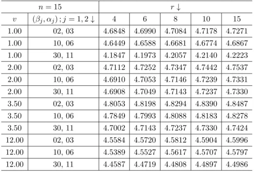
4 Numerical Analysis (Shape Parameter Known)
To assess and study the properties of the Bayes estimators for shift point m when the shape parameter v is known, a simulation study has been carried out. The random samples are generated as follows:
1. Generateθ1 and θ2 through prior densityg1(θ1) andg2(θ2) for the given values of
prior parameters αj and βj as (αj, βj) = (03,02),(06,10),(11,30) , j = 1,2. The
value of αj and βj are chosen so as to keep the prior variance unity.
2. Using θ1 and θ2 obtained in (1), and the considered values of shape parameter
v= 1.00,2.00,3.50,12.00; generate the 10,000 random samples of sizen= 15 from the model (2) and (4).
3. Here the value of v= 1.00 and 2.00 should meet the criterion for the Exponential and Rayleigh distribution respectively. Similarly others two values make the shape of the distribution close to that of Normal and smallest extreme value distribution respectively.
4. For the selected set of censored sample size r = 04,06,08,10; the values of the Bayes estimate and posterior risk for the shift point under the SELF have been obtained and presented in the Table 01 - 02.
5. It is observed here that when censored sample size r increases the magnitude of the Bayes estimator increases but the increment in magnitude is nominal (robust). 6. A decreasing trend has been seen when (αj, βj) increases.
7. It is also noted that when the values of the shape parameterv increases the mag-nitude of the Bayes estimator also increases, however for large value of shape pa-rameterv (say 12) i.e., for the smallest extreme value distribution the magnitude of the Bayes estimator decreases.
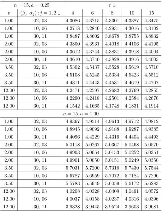
8. With considered set of values and a= 0.25,0.50,1.00,2.00; the magnitude of the Bayes estimator under LLF and posterior risk have been obtained and presented in the Table 03 - 04, only fora= 0.25,1.00.
9. Similar properties as discussed above have been seen for the Bayes estimate of the shift point ˆmL.Further, an increasing trend in the magnitude of the estimate
also has been seen when 0a0 increases (except for large v) but the increment in magnitude is robust.
10. It observed from tables that the magnitudes of posterior risk are smaller and nominal. Other properties are seen to be similar as discussed above.
Remark:
In the case when the censored sample size r = 15; the censoring criterion is reduces to the complete sample size criterion and hence the result are valid for complete sample case.
5 Bayes Estimator of Shift Point (Shape Parameter
Unknown)
When both of the parameters θ and v of the considered model (1) are unknown, there do not exist any joint conjugate prior distribution. One of the good choices of the joint prior distribution when both parameters are unknown is given by
The prior distributionsg(θ|v) and f(v) are defined as g(θ|v) = v α Γ(α) θ −(α+1)exp−v θ ; α >0, v >0, θ >0 and f(v) = b c Γ(c) θ −(c+1)exp −b v ; b >0, c >0, v >0.
When both parameters are considered to be unknown, the likelihood function is given as L θ1, θ2, v, m|x(1), x(2), ..., x(r) = v r θ1mθr2−m r Y i=1 xv(i)−1 ! exp −δ1 θ1 −δ2 θ2 . (20)
The joint prior distribution is now defined as
h1(θ1, θ2, v, m)∝g1(θ1|v) . g2(θ2|v) . f(v). g3(m) ; wheregj(θj|v) = v αj Γ(αj) θ −(αj+1) j exp −θv j ; αj >0, v >0, θj >0, j= 1,2.
Thus, the joint posterior density is obtained as
Z1(θ1, θ2, v, m) = 1 K1 L θ1, θ2, v, m|x(1), x(2), ..., x(r) . h1(θ1, θ2, v, m) whereK1 =Pm R v R θ1 R θ2 L θ1, θ2, v, m|x(1), x(2), ..., x(r) .h1(θ1, θ2, v, m).dθ2.dθ1.dv
After simplification the joint posterior density is
Z1(θ1, θ2, v, m) = ¯Φθ1−(m+α1+1)θ−2(r−m+α2+1)ξ(v)exp −ω3 θ1 −ω4 θ2 ; (21) where ¯Φ =P m∆¯¯ −1 ,∆ =¯¯ R vξ(v) ¯∆dv,∆ =¯ Γ(m+α1) Γ(r−m+α2) ωm+α1 3 ω r−m+α2 4 , ξ(v) =vr+α1+α2−c−1 Qr i=1x v−1 (i) exp − b v and ωj+2 =v+δj;j= 1,2.
The marginal posterior density for shift point m in present case is obtain as
Z1∗(m) = Z θ1 Z θ2 Z v Z1(θ1, θ2, v, m) dv. dθ2. dθ1 ⇒Z1∗(m) = ¯φ∆¯¯. (22)
The Bayes estimator for the shift point estimator m under the SELF is ˆ mS1= ¯φ X m m∆¯¯ . (23)
Similarly, the Bayes estimator for the shift point under the LLF is given by ˆ mL1=− 1 aln ( ¯ φX m e−am∆¯¯ ) . (24)
The posterior risk for Bayes estimators ˆmS1and ˆmL1are obtained similarly as in known
shape parameter case.
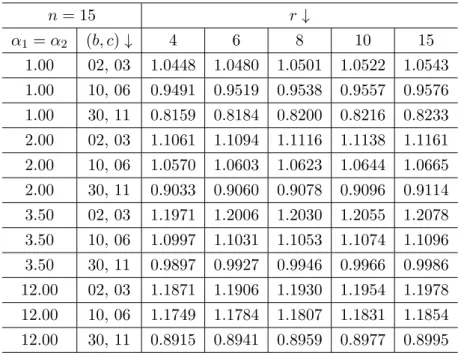
6 Numerical Analysis (Shape Parameter Unknown)
When both parameters are considered as the random variable, a simulation study also has been carried out to study the properties of the Bayes estimators for shift point as follows:
1. Generate the values of the shape parameter v through prior density f(v) for the given set of values (c, b) = (03,02),(06,10),(11,30).The value ofcandbare chosen so as to keep the prior variance unity.
2. Using the generated values of v in (1), we generate the values ofθ1 and θ2 for the
previous selected values of prior parameter.
3. Using above generated values of θ1, θ2 and v obtained in steps (1) & (2), generate
the 10,000 random samples of sizen= 15 form the considered model.
4. The values of Bayes estimate ˆmS1 for shift point under SELF and Posterior risk
has been obtain for censored sample sizer= 04,06,08,10,and presented in Tables 05 - 06.
5. All the properties are seen similar as compared to ˆmS (known shape parameter
case).
6. Using similar set of parametric values as discussed earlier, the magnitude of Bayes estimator ˆmL1 under LLF and Posterior risk have been obtained and presented in
Tables 07 - 08, only fora= 0.25,1.00.
7. An increasing trend in the magnitude of the estimate also has been seen when0a0
increases but the increment in magnitude is least (robust). Others properties are similar as in case of known shape parameter.
8. Both the estimators are robust and the magnitudes of posterior risk are least. Other properties are seen to be similar as discussed above
7 Sensitivity of Bayes Estimates
Following Calabria and Pulcini (1996), we study the sensitivity of the Bayes estimator with respect to change in prior of parameters. The prior mean and prior variance
µj, σ2j ; j= 1,2
have been used as the prior information in computing the hyper -parameters of the prior distribution. The sensitivity analysis is based on assumption that the prior information to be correct if the true value of the parameters θ1(θ2) is
close to prior mean µ1(µ2) and is assumed to be wrong if the parameters θ1(θ2) is far
from the prior mean µ1(µ2). For this, we have computed the posterior mean for the
selected set of parameters as discussed in section 4 and presented in Table 09. It is seen from the table that the posterior mean appears to be robust with respect to the correct choice as well as wrong choice of the prior density of θ1(θ2).
8 Conclusion
Two parameter Weibull distribution is consider here as the underlying model for the study. The study of shift point estimation for the Weibull model is performing under the Bayesian approach. The censoring criteria inside the shift point estimation have been proposed first time in present article. Both known and unknown case of shape parameter is considered here for the study of Bayes estimation of the shift point under the symmetric and asymmetric loss function.
A simulation study has been carried out for the study of the properties of the Bayes estimation. Based on the findings the magnitude of the estimator is robust. It is also observed that when the value of the shape parameter of LLF is small the difference between the magnitudes of Bayes estimates under SELF and LLF is robust.
Table 1: Bayes Estimate of ˆmS (Shape Parameter Known) n= 15 r↓ v (βj, αj) ;j= 1,2↓ 4 6 8 10 15 1.00 02, 03 4.6848 4.6990 4.7084 4.7178 4.7271 1.00 10, 06 4.6449 4.6588 4.6681 4.6774 4.6867 1.00 30, 11 4.1847 4.1973 4.2057 4.2140 4.2223 2.00 02, 03 4.7112 4.7252 4.7347 4.7442 4.7537 2.00 10, 06 4.6910 4.7053 4.7146 4.7239 4.7331 2.00 30, 11 4.6908 4.7049 4.7143 4.7237 4.7330 3.50 02, 03 4.8053 4.8198 4.8294 4.8390 4.8487 3.50 10, 06 4.7849 4.7993 4.8088 4.8183 4.8278 3.50 30, 11 4.7002 4.7143 4.7237 4.7330 4.7424 12.00 02, 03 4.5584 4.5720 4.5812 4.5904 4.5996 12.00 10, 06 4.5389 4.5527 4.5617 4.5707 4.5797 12.00 30, 11 4.4587 4.4719 4.4808 4.4897 4.4986
Table 2: Posterior Risk for ˆmS (Shape Parameter Known)
n= 15 r↓ v (βj, αj) ;j= 1,2↓ 4 6 8 10 15 1.00 02, 03 1.6709 1.6758 1.6792 1.6826 1.6860 1.00 10, 06 1.6133 1.6182 1.6214 1.6246 1.6278 1.00 30, 11 1.5352 1.5398 1.5428 1.5459 1.5490 2.00 02, 03 1.7614 1.7667 1.7702 1.7737 1.7773 2.00 10, 06 1.7007 1.7058 1.7092 1.7126 1.7160 2.00 30, 11 1.6184 1.6232 1.6265 1.6297 1.6329 3.50 02, 03 1.7640 1.7694 1.7729 1.7765 1.7800 3.50 10, 06 1.7142 1.7195 1.7229 1.7263 1.7296 3.50 30, 11 1.6620 1.6670 1.6704 1.6737 1.6770 12.00 02, 03 1.7740 1.7792 1.7828 1.7864 1.7900 12.00 10, 06 1.6974 1.7025 1.7059 1.7093 1.7127 12.00 30, 11 1.4827 1.4872 1.4902 1.4931 1.4960
Table 3: Bayes Estimate of ˆmL (Shape Parameter Known) n= 15, a= 0.25 r↓ v (βj, αj) ;j= 1,2↓ 4 6 8 10 15 1.00 02, 03 4.3086 4.3215 4.3301 4.3387 4.3475 1.00 10, 06 4.2718 4.2846 4.2931 4.3016 4.3102 1.00 30, 11 3.8487 3.8602 3.8678 3.8755 3.8832 2.00 02, 03 4.3800 4.3931 4.4018 4.4106 4.4195 2.00 10, 06 4.3612 4.3744 4.3831 4.3918 4.4004 2.00 30, 11 4.3610 4.3740 4.3828 4.3916 4.4003 3.50 02, 03 4.5302 4.5437 4.5528 4.5619 4.5710 3.50 10, 06 4.5108 4.5245 4.5334 4.5423 4.5512 3.50 30, 11 4.4311 4.4443 4.4531 4.4619 4.4707 12.00 02, 03 4.2471 4.2597 4.2682 4.2769 4.2855 12.00 10, 06 4.2290 4.2418 4.2501 4.2584 4.2670 12.00 30, 11 4.1542 4.1665 4.1748 4.1831 4.1914 n= 15, a= 1.00 1.00 02, 03 4.9367 4.9514 4.9613 4.9712 4.9812 1.00 10, 06 4.8945 4.9092 4.9188 4.9287 4.9385 1.00 30, 11 4.4096 4.4229 4.4316 4.4404 4.4493 2.00 02, 03 5.0118 5.0267 5.0367 5.0468 5.0570 2.00 10, 06 4.9903 5.0054 5.0153 5.0252 5.0351 2.00 30, 11 4.9901 5.0050 5.0151 5.0249 5.0350 3.50 02, 03 5.7031 5.7200 5.7316 5.7430 5.7544 3.50 10, 06 5.6787 5.6959 5.7072 5.7184 5.7296 3.50 30, 11 5.5783 5.5949 5.6059 5.6172 5.6283 12.00 02, 03 4.0208 4.0328 4.0409 4.0491 4.0572 12.00 10, 06 4.0037 4.0158 4.0237 4.0316 4.0396 12.00 30, 11 3.9328 3.9445 3.9524 3.9603 3.9681
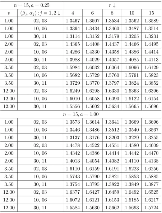
Table 4: Posterior Risk for ˆmL (Shape Parameter Known) n= 15, a= 0.25 r↓ v (βj, αj) ;j= 1,2↓ 4 6 8 10 15 1.00 02, 03 1.3467 1.3507 1.3534 1.3562 1.3589 1.00 10, 06 1.3394 1.3434 1.3460 1.3487 1.3514 1.00 30, 11 1.3114 1.3152 1.3179 1.3205 1.3231 2.00 02, 03 1.4365 1.4408 1.4437 1.4466 1.4495 2.00 10, 06 1.4286 1.4330 1.4358 1.4386 1.4414 2.00 30, 11 1.3988 1.4029 1.4057 1.4085 1.4113 3.50 02, 03 1.5984 1.6032 1.6064 1.6096 1.6129 3.50 10, 06 1.5682 1.5729 1.5760 1.5791 1.5823 3.50 30, 11 1.3729 1.3770 1.3797 1.3824 1.3852 12.00 02, 03 1.6249 1.6298 1.6330 1.6363 1.6396 12.00 10, 06 1.6010 1.6058 1.6090 1.6122 1.6154 12.00 30, 11 1.5556 1.5602 1.5634 1.5665 1.5696 n= 15, a= 1.00 1.00 02, 03 1.3573 1.3614 1.3641 1.3669 1.3696 1.00 10, 06 1.3446 1.3486 1.3512 1.3540 1.3567 1.00 30, 11 1.3137 1.3176 1.3203 1.3229 1.3255 2.00 02, 03 1.4478 1.4522 1.4551 1.4580 1.4609 2.00 10, 06 1.4342 1.4386 1.4414 1.4442 1.4470 2.00 30, 11 1.4013 1.4054 1.4082 1.4110 1.4138 3.50 02, 03 1.6110 1.6159 1.6191 1.6223 1.6256 3.50 10, 06 1.5743 1.5790 1.5821 1.5853 1.5885 3.50 30, 11 1.3754 1.3795 1.3822 1.3849 1.3877 12.00 02, 03 1.6377 1.6427 1.6459 1.6492 1.6525 12.00 10, 06 1.6072 1.6121 1.6153 1.6185 1.6217 12.00 30, 11 1.5584 1.5630 1.5662 1.5693 1.5724
Table 5: Bayes Estimate of ˆmS1 (Shape Parameter Unknown) n= 15 r↓ α1=α2 (b, c)↓ 4 6 8 10 15 1.00 02, 03 4.3800 4.3932 4.4019 4.4108 4.4195 1.00 10, 06 4.3427 4.3556 4.3643 4.3730 4.3817 1.00 30, 11 3.9125 3.9242 3.9320 3.9398 3.9476 2.00 02, 03 4.4502 4.4635 4.4725 4.4814 4.4904 2.00 10, 06 4.4312 4.4447 4.4534 4.4622 4.4709 2.00 30, 11 4.4310 4.4443 4.4531 4.4620 4.4708 3.50 02, 03 4.6300 4.6438 4.6531 4.6625 4.6717 3.50 10, 06 4.6102 4.6241 4.6333 4.6424 4.6516 3.50 30, 11 4.5287 4.5422 4.5511 4.5602 4.5693 12.00 02, 03 4.2618 4.2745 4.2830 4.2917 4.3002 12.00 10, 06 4.2436 4.2564 4.2648 4.2732 4.2817 12.00 30, 11 4.1685 4.1810 4.1892 4.1976 4.2060
Table 6: Posterior Risk for ˆmS1 (Shape Parameter Unknown)
n= 15 r↓ α1=α2 (b, c)↓ 4 6 8 10 15 1.00 02, 03 1.0448 1.0480 1.0501 1.0522 1.0543 1.00 10, 06 0.9491 0.9519 0.9538 0.9557 0.9576 1.00 30, 11 0.8159 0.8184 0.8200 0.8216 0.8233 2.00 02, 03 1.1061 1.1094 1.1116 1.1138 1.1161 2.00 10, 06 1.0570 1.0603 1.0623 1.0644 1.0665 2.00 30, 11 0.9033 0.9060 0.9078 0.9096 0.9114 3.50 02, 03 1.1971 1.2006 1.2030 1.2055 1.2078 3.50 10, 06 1.0997 1.1031 1.1053 1.1074 1.1096 3.50 30, 11 0.9897 0.9927 0.9946 0.9966 0.9986 12.00 02, 03 1.1871 1.1906 1.1930 1.1954 1.1978 12.00 10, 06 1.1749 1.1784 1.1807 1.1831 1.1854 12.00 30, 11 0.8915 0.8941 0.8959 0.8977 0.8995
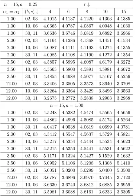
Table 7: Bayes Estimate of ˆmL1 (Shape Parameter Unknown) n= 15, a= 0.25 r↓ α1=α2 (b, c)↓ 4 6 8 10 15 1.00 02, 03 4.1015 4.1137 4.1220 4.1303 4.1385 1.00 10, 06 4.0665 4.0787 4.0867 4.0948 4.1030 1.00 30, 11 3.6636 3.6746 3.6819 3.6892 3.6966 2.00 02, 03 4.1164 4.1286 4.1368 4.1451 4.1534 2.00 10, 06 4.0987 4.1111 4.1193 4.1274 4.1355 2.00 30, 11 4.0985 4.1108 4.1190 4.1272 4.1354 3.50 02, 03 4.5857 4.5995 4.6087 4.6179 4.6272 3.50 10, 06 4.5663 4.5800 4.5891 4.5981 4.6072 3.50 30, 11 4.4855 4.4988 4.5077 4.5167 4.5256 12.00 02, 03 3.3406 3.3505 3.3573 3.3640 3.3708 12.00 10, 06 3.3264 3.3364 3.3429 3.3496 3.3563 12.00 30, 11 3.2675 3.2772 3.2838 3.2903 3.2968 n= 15, a= 1.00 1.00 02, 03 4.5248 4.5382 4.5474 4.5565 4.5656 1.00 10, 06 4.4862 4.4996 4.5085 4.5174 4.5264 1.00 30, 11 4.0417 4.0538 4.0619 4.0699 4.0781 2.00 02, 03 4.5412 4.5547 4.5637 4.5729 4.5821 2.00 10, 06 4.5217 4.5354 4.5444 4.5534 4.5623 2.00 30, 11 4.5215 4.5350 4.5441 4.5531 4.5622 3.50 02, 03 5.1171 5.1324 5.1427 5.1529 5.1632 3.50 10, 06 5.0952 5.1106 5.1208 5.1308 5.1410 3.50 30, 11 5.0051 5.0200 5.0299 5.0400 5.0500 12.00 02, 03 3.6787 3.6896 3.6970 3.7045 3.7120 12.00 10, 06 3.6630 3.6740 3.6812 3.6885 3.6959 12.00 30, 11 3.5981 3.6088 3.6161 3.6233 3.6305
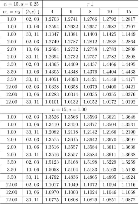
Table 8: Posterior Risk for ˆmL1 (Shape Parameter Unknown) n= 15, a= 0.25 r↓ α1=α2 (b, c)↓ 4 6 8 10 15 1.00 02, 03 1.2703 1.2741 1.2766 1.2792 1.2817 1.00 10, 06 1.2594 1.2632 1.2657 1.2682 1.2707 1.00 30, 11 1.1347 1.1381 1.1403 1.1425 1.1449 2.00 02, 03 1.2749 1.2787 1.2812 1.2838 1.2864 2.00 10, 06 1.2694 1.2732 1.2758 1.2783 1.2808 2.00 30, 11 1.2694 1.2732 1.2757 1.2782 1.2808 3.50 02, 03 1.4365 1.4409 1.4437 1.4466 1.4495 3.50 10, 06 1.4305 1.4348 1.4376 1.4404 1.4433 3.50 30, 11 1.4051 1.4093 1.4121 1.4149 1.4177 12.00 02, 03 1.0328 1.0358 1.0379 1.0400 1.0421 12.00 10, 06 1.0283 1.0314 1.0335 1.0355 1.0376 12.00 30, 11 1.0101 1.0132 1.0152 1.0172 1.0192 n= 15, a= 1.00 1.00 02, 03 1.3526 1.3566 1.3593 1.3621 1.3648 1.00 10, 06 1.3410 1.3450 1.3477 1.3504 1.3531 1.00 30, 11 1.2082 1.2118 1.2142 1.2166 1.2190 2.00 02, 03 1.3575 1.3615 1.3642 1.3670 1.3697 2.00 10, 06 1.3516 1.3557 1.3584 1.3611 1.3638 2.00 30, 11 1.3516 1.3557 1.3584 1.3611 1.3638 3.50 02, 03 1.5123 1.5168 1.5198 1.5229 1.5259 3.50 10, 06 1.5058 1.5104 1.5133 1.5163 1.5193 3.50 30, 11 1.4792 1.4836 1.4865 1.4895 1.4924 12.00 02, 03 1.1017 1.1049 1.1072 1.1094 1.1116 12.00 10, 06 1.0970 1.1003 1.1024 1.1046 1.1068 12.00 30, 11 1.0775 1.0808 1.0829 1.0851 1.0872
Table 9: Estimate of Posterior Mean n= 15 Posterior Mean µ1 µ2 4 6 8 10 1.00 1.00 6.9851 7.9328 8.2158 9.3305 2.00 2.00 6.9855 7.9333 8.2163 9.3311 3.00 3.00 6.9862 7.9341 8.2169 9.3317
References
Arnold, B. C. and Press, S. J. (1983). Bayesian inference for pareto populations. Journal of Econometrics, 21:287–306.
Berrettoni, J. A. (1964). Practical applications of the weibull distribution. Industrial Quality Control, 21:71–79.
Broemeling, L. D. and Tsurumi, H. (1987). Econometrics and structural change. Marcel Dekker, New York.
Calabria, R. and Pulcini, G. (1996). Point estimation under asymmetric loss functions for left - truncated exponential samples. Communication in Statistics - Theory and Methods, 25(3):585–600.
Chandra, N. K. and Chaudhari, A. (1990). On testing the weibull shape parameter.
Communications in Statistics - Computation and Simulation, 19(2):637–648.
Ebrahimi, N. and Ghosh, S. K. (2001). Bayesian and frequentist methods in change -point problems. Handbook of statistics: Advance in Reliability, Eds. N. Balakrishna & C. R. Rao, 20:777–787.
Jani, P. N. and Pandya, M. (1999). Bayes estimation of shift point in left truncated ex-ponential sequence. Communications in Statistics - Theory and Methods, 28(11):2623– 2639.
Kao, J. H. K. (1959). A graphical estimation of mixed weibull parameters in life testing electron tubes. Technometrics, 4:309–407.
Lieblein, J. and Zelen, M. (1956). Statistical investigation of the fatigue life of deep groove ball bearings. Journal of Research: National Bureau of Standards, 57:273–315. Mittnik, S. and Rachev, S. T. (1993). Modeling asset returns with alternative stable
distribution. Economic Reviews, 12:261–330.
Nelson, W. B. (1972). Graphical analysis of accelerated life test data with the inverse power law model. IEEE Transaction on Reliability, 21(R):2–11.
Pandey, B. N., Malik, H. J., and Srivastava, R. (1989). Shrinkage testimators for the shape parameter of weibull distribution under type - ii censoring. Communications in Statistics - Theory and Methods, 18(6):1175–1199.
Pandey, M. (1983). Shrunken estimators of weibull shape parameter in censored samples.
IEEE Transactions on Reliability, 32(R):200–202.
Pandya, M. and Jadav, P. (2010). Bayesian estimation of change point in mixture of left truncated exponential and degenerate distribution. Communication in statistics -Theory and Methods, 39(15):2725–2742.
Parsian, A. and Kirmani, S. N. U. A. (2002). Estimation under linex loss function, in: A. ullah, a. t. k. wan, a. chaturvedi & m. dekker, eds. Handbook of Applied Econometrics and Statistical Inference, CRC Press, Boca Raton, pages 53–76.
Prakash, G. and Singh, D. (2008). Item failure data of weibull failure model under bayesian estimation. Journal of Statistical Research, 42(2):131–140.
failure censored sampling under the linex loss. METRON - International Journal of Statistics, 37(1):31–50.
Singh, D. C., Prakash, G., and Singh, P. (2007). Shrinkage testimators for the shape pa-rameter of pareto distribution using linex loss function. Communications in Statistics - Theory and Methods, 36(6):741–753.
Singh, H. P. and Shukla, S. K. (2000). Estimation in the two - parameters weibull distribution with prior information. IAPQR Transactions, 25(2):107–118.
Tsionas, E. G. (2002). Bayesian analysis of finite mixtures of weibull distributions.
Communications in Statistics - Theory and Methods, 31(1):37–48.
Wahed, A. S., Luong, T. M., and Jeong, J. H. (2009). A new generalization of weibull distribution with application to a breast cancer data set. Statistical Medicine, 28(16):2077–2094.
Weibull, W. (1951). A statistical distribution functions of wide applicability. Journal of Applied Mathematics and Mechanics, 18:293–297.
Whittemore, A. and Altschuler, B. (1976). Lung cancer incidence in cigarette smokes: further analysis of the doll and hill’s data for british physicians. Biometrics, 32:805– 816.