Detection and Localisation Using Light

(1)

Detection and Localisation

Using Light

Aubida Abdulwahab Jasim Al-Hameed

Submitted in accordance with the requirements for the

degree of Doctor of Philosophy

School of Electronic and Electrical Engineering

March 2019

(2)

where work which has formed part of jointly authored publications

has been included. The contribution of the candidate and the other

authors to this work has been explicitly indicated below. The

candidate confirms that appropriate credit has been given within

the thesis where reference has been made to the work of others.

The work in Chapter 3, 4, 5, 6 and 7 of the thesis has appeared

in publications as follows:

1. Aubida A. Al-Hameed, Safwan Hafeedh Younus, Ahmed Taha Hussein, Mohammed T. Alresheedi and Jaafar M. H. Elmirghani, “LiDAL: Light Detection and Localisation,” IEEE Access, submitted March 2019.

- My contribution: literature review, developed the idea, produced results and wrote the work.

- Professor Jaafar M. H. Elmirghani suggested the paper idea, supervised and revised the work.

- Dr. Safwan Hafeedh Younus, Dr. Ahmed Taha Hussein and Dr. Mohammed T. Alresheedi helped with the revision of the work.

This copy has been supplied on the understanding that it is

copyright material and that no quotation from the thesis may be

published without proper acknowledgement.

(3)

(4)

i

Acknowledgements

First and foremost, all praise to Almighty Allah, for endowing me with health, patience, and knowledge to complete this work. I would like to acknowledge my supervisor, Professor Jaafar Elmirghani for his guidance and patience through my PhD journey. I am grateful for his teachings, guidance and support. He has offered me invaluable opportunities and continuously kept faith in me.

I am very grateful and thankful to the Higher Committee for Education Development (HCED) in Iraq for fully funding my PhD.

Many thanks go to my colleagues in the Communication Systems and Networks group in the School of Electronic and Electronic Engineering at University of Leeds. Also, I send my special thanks to Dr. Ahmed T. Hussein Dr. Safwan H. Younus and Dr. Mohamed Musa. It was a privilege to have known them. I thank them for their company, reassurance and fruitful discussions.

I would like to express my appreciation to my beloved family back home, my mother, sister and brother. I don’t have enough words to thank them for supporting me in all possible ways. They are the reason behind my life achievements and have always shown me by example that everything is doable. I hope I made them proud.

(5)

ii

Abstract

Visible light communication (VLC) systems have become promising candidates to complement conventional radio frequency (RF) systems due to the increasingly saturated RF spectrum and the potentially high data rates that can be achieved by VLC systems. Furthermore, people detection and counting in an indoor environment has become an emerging and attractive area in the past decade. Many techniques and systems have been developed for counting in public places such as subways, bus stations and supermarkets. The outcome of these techniques can be used for public security, resource allocation and marketing decisions.

This thesis presents the first indoor light-based detection and localisation system that builds on concepts from radio detection and ranging (radar) making use of the expected growth in the use and adoption of visible light communication (VLC), which can provide the infrastructure for our light detection and localisation (LiDAL) system. Our system enables active detection, counting and localisation of people, in addition to being fully compatible with existing VLC systems. In order to detect human (targets), LiDAL uses the visible light spectrum. It sends pulses using a VLC transmitter and analyses the reflected signal collected by an optical receiver. Although we examine the use of the visible spectrum here, LiDAL can be used in the infrared spectrum and other parts of the light spectrum.

We introduce LiDAL with different transmitter-receiver configurations and optimum detectors considering the fluctuation of the received reflected signal from the target in the presence of Gaussian noise. We design an efficient multiple input multiple output (MIMO) LiDAL system with wide field of view (FOV) single photodetector receiver, and also design a multiple input single output (MISO) LiDAL system with an imaging receiver to eliminate ambiguity in target detection and localisation.

We develop models for the human body and its reflections and consider the impact of the colour and texture of the cloth used as well as the impact of target mobility. A number of detection and localisation methods are developed

(6)

iii

method and a background estimation method. These methods are considered to distinguish a mobile target from the ambient reflections due to background obstacles (furniture) in a realistic indoor environment.

(7)

iv

List of Figures

Figure 2.1 Block diagram of VLC system. ... 26

Figure 2.2: Non-directional hemispherical lens that employs a planar filter [53]. ... 29

Figure 2.3: Compound parabolic concentrator [53]. ... 29

Figure 2.4: Relative spectral power densities of the three common ambient light sources [53]. ... 30

Figure 2.5: Ray tracing setup for LOS, first and second order reflections [93], [94]. ... 37

Figure 2.6: Ray tracing for LOS [94]. ... 38

Figure 2.7: Ray tracing for first order reflections [94]. ... 39

Figure 2.8: Radar system setup. ... 43

Figure 2.9:(a) Bistatic radar configuration and (b) Monostatic radar configuration... 45

Figure 2.10: Block diagram of LiDAR system with (a) incoherent detection and (b) coherent detection. ... 49

Figure 3.1: Realistic office room setup. ... 57

Figure 3.2: Basic 3D and 2D target model. ... 57

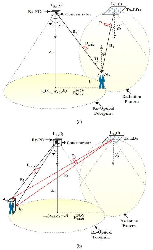
Figure 3.3: (a) a spaced transmitter-receiver (bistatic) placed on room ceiling with a target located near by the transmitter and distance of 𝑅MaxFOV from the receiver (b) a spaced transmitter-receiver placed on room ceiling with a target located away from the ... 61

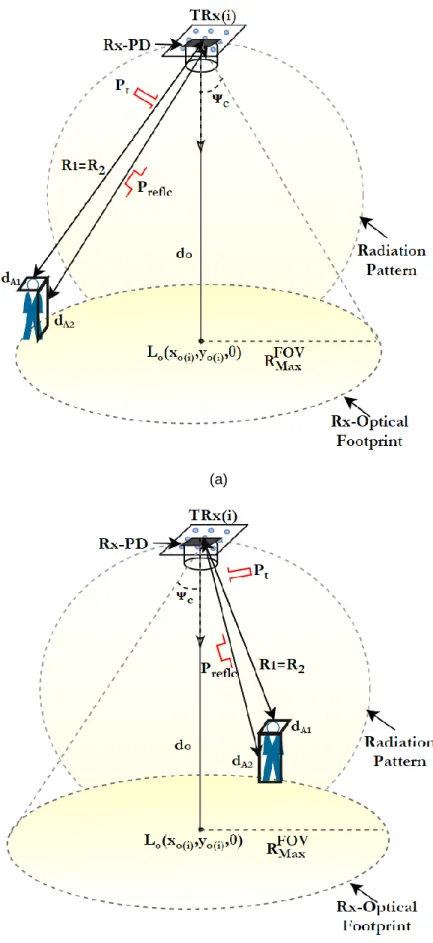
Figure 3.4: (a) and (b) a collocated transmitter-receiver (monostatic) placed on room ceiling with a target at two different locations. ... 62

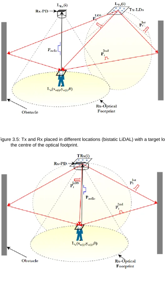
Figure 3.5: Tx and Rx placed in different locations (bistatic LiDAL) with a target located in the centre of the optical footprint... 64

Figure 3.6:Tx and Rx placed in same location (monostatic LiDAL ) a target located in the centre of the optical footprint... 64

(11)

viii

x=2.5m, y=5m, (b) Bistatic LiDAL impulse response of target located at x=2m, y=3m and (c) the PDF of the Bistatic LiDAL

channel bandwidth. ... 66

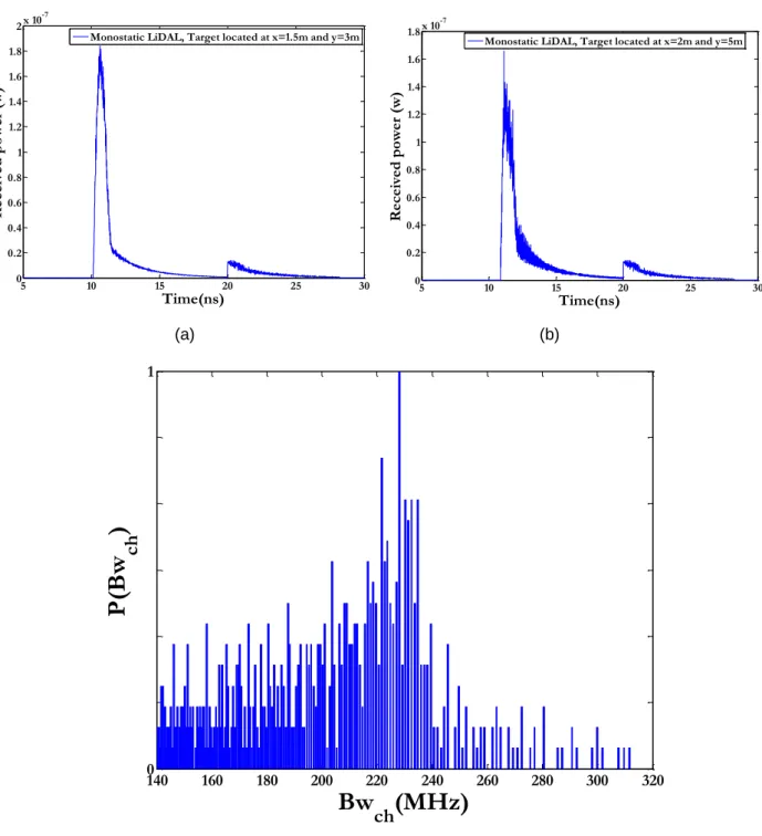
Figure 3.8: (a) Monostatic LiDAL impulse response of target located at x=1.5m, y=3m, (b) Monostatic LiDAL impulse response of target located at x=2m, y=5m and (c) the PDF of the monostatic LiDAL channel bandwidth. ... 67

Figure 3.9: The LiDAL resolution to distinguish two targets. ... 70

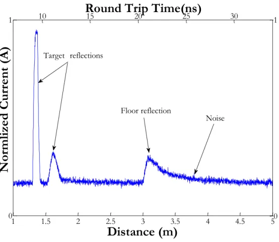
Figure 3.10: The reflected received current signal from two targets located in empty room of monostatic LiDAL. ... 71

Figure 3.11: The PDF of target reflection factor. ... 73

Figure 3.12: The PDF of the effective target cross section area. ... 75

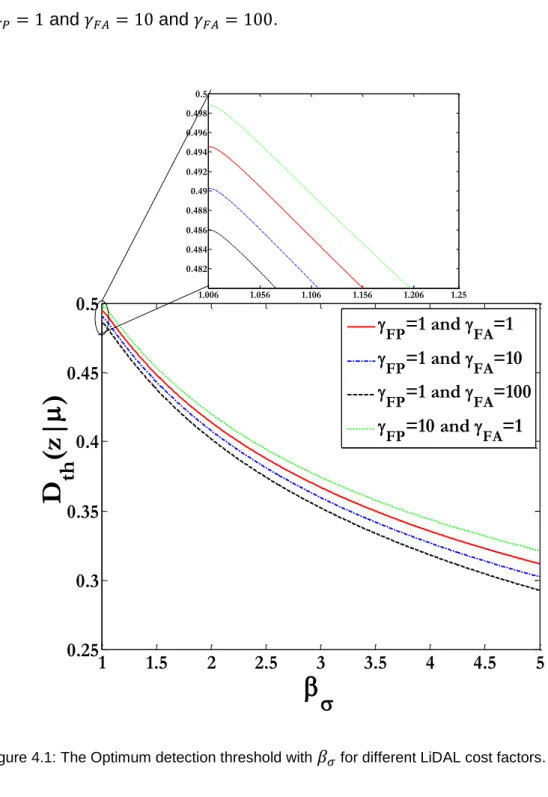
Figure 4.1: The Optimum detection threshold with 𝛽𝜎 for different LiDAL cost factors. ... 83

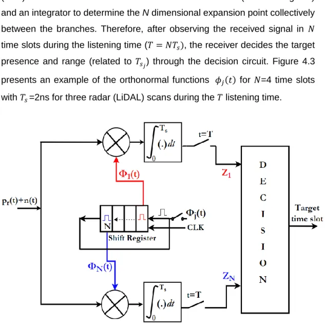
Figure 4.2: The LiDAL optimum detector block diagram, single target detection. ... 89

Figure 4.3: The orthonormal 𝝓𝒋𝒕 signalling diagram. ... 90

Figure 4.4: The LiDAL sub-optimum receiver block diagram. ... 94

Figure 4.5: The LiDAL receiver two-dimensional observation space. ... 95

Figure 4.6: Probability of error of detecting targets for ESR and SOR. ... 99

Figure 5.1: BSM of the received snapshots measurements. ... 105

Figure 5.2: Receiver block diagram of LiDAL with BSM. ... 105

Figure 5.3: LiDAL snapshots measurement cube. ... 107

Figure 5.4: (a) received reflected signals in two snapshots measurement in Proposition I and (b) CCM of received snapshots measurement of Proposition I. ... 109

Figure 5.5: (a) received reflected signals in two snapshots measurement in Proposition II and (b) CCM of received snapshots measurement of Proposition II. ... 111

Figure 5.6: : (a) received reflected signals in two snapshots measurement in Proposition III and (b) CCM of received snapshots measurement of Proposition III. ... 113

Figure 5.7:(a) received reflected signals in two snapshots measurement in Proposition IV and (b) CCM of received snapshots measurement of Proposition IV. ... 114

Figure 5.8: LiDAL receiver block diagram with CCM. ... 118

Figure 5.9: Target random walk model in 𝑮(𝒙, 𝒚) space. ... 121

Figure 5.10: Probability of target mobility detection in a realistic environment. ... 123

(12)

ix

Figure 5.12: LiDAL receiver block diagram with BEM. ... 128

Figure 5.13: Simulation room setup with Monostatic LiDAL. ... 129

Figure 5.14: False target distinguishing error in static environment. ... 130

Figure 5.15: False target distinguishing error in dynamic environment. .... 132

Figure 6.1:MIMO-LiDAL system setup. ... 139

Figure 6.2: MIMO monostatic LiDAL. ... 140

Figure 6.3: ROC of Monostatic MIMO LiDAL. ... 142

Figure 6.4:Monostatic MIMO LiDAL false detection with optimum 𝑫𝒕𝒉𝑴. ... 142

Figure 6.5: Target detection ambiguity in MIMO-LiDAL system with targets ranging ... 144

Figure 6.6:(a) the reflected pulses from targets when Tx1-Rx1 are active, (b) the reflected pulses from targets when Tx2-Rx1 are active and (c) the reflected pulses from targets when Tx3-Rx1 are active. ... 145

Figure 6.7:Bistatic MIMO LiDAL system. ... 146

Figure 6.8:ROC of Bistatic MIMO LiDAL. ... 148

Figure 6.9: Bistatic MIMO LiDAL probability of false detection with optimum 𝑫𝒕𝒉𝑩. ... 148

Figure 6.10: The receiver block diagram of MIMO-LiDAL system. ... 154

Figure 6.11: MIMO LiDAL Room A setup in scenario 1. ... 157

Figure 6.12 MIMO LiDAL Room B setup in scenario 2. ... 157

Figure 6.13: MAPE of MIMO LiDAL system with BSM and CCM in Room A of scenario 1. ... 163

Figure 6.14: MAPE of MIMO LiDAL system with BSM and CCM in Room B of scenario 2. ... 164

Figure 6.15: CDF of DRMSE of the proposed MIMO LiDAL system. ... 165

Figure 6.16: CDF of counting MAPE in the MIMO LiDAL system for nomadic targets with different MF. ... 167

Figure 7.1: MISO-IMG-LiDAL system. ... 171

Figure 7.2: LiDAL imaging receiver design, lens FOV with 𝑹𝑴𝒂𝒙𝑭𝑶𝑽. .... 172

Figure 7.3: targets optical resolution in MISO IMG LiDAL system. ... 173

Figure 7.4: Pixel’s angles of IMG LiDAL system. ... 175

Figure 7.5:Bistatic MISO-IMG-LiDAL system. ... 177

Figure 7.6: ROC of Bistatic MISO -IMG-LiDAL system. ... 178

Figure 7.7: Bistatic MISO-IMG-LiDAL false detection with optimum 𝐷𝑡ℎ𝐵𝑖𝑚𝑔. ... 178

(13)

x

Figure 7.9:A top view of three targets movement on the detection floor

of MISO-IMG- LiDAL system during S snapshots measurements. .... 183

Figure 7.10: Eight GRPs of the imaging receiver. ... 186

Figure 7.11: The proposed sub-optimum imaging receiver (SOIMR) for IMG LiDAL system. ... 186

Figure 7.12:the receiver block diagram of MISO-IMG-LiDAL. ... 187

Figure 7.13: MISO IMG LiDAL Room A setup in scenario 1. ... 190

Figure 7.14: MISO IMG LiDAL Room A setup in scenario 2. ... 190

Figure 7.15: MAPE of LiDAL systems with BSM and CCM in empty environment of scenario 1. ... 192

Figure 7.16: MAPE of LiDAL systems with BSM and CCM in realistic environment of scenario 2. ... 193

Figure 7.17: CDFs of DRMSE of the proposed LiDAL systems. ... 194

Figure 7.18: MISO-IMG LiDAL system MAPE CDF for the nomadic targets with different MF. ... 195

Figure 7.19: CDF of counting MAPE in the MIMO LiDAL system for nomadic targets with different MF. ... 196

Figure 7.20: CDF of counting MAPE of the targets, when the targets move along fixed pathways. ... 199

Figure 7.21: CDF of counting MAPE of the targets, when the targets move following a random walk model. ... 201

List of Tables

Table 3.1:Reflection model for a different target coating materials [152]... 56

Table 3.2: Characteristic of LiDAL Channel. ... 66

Table 3.3: Popular Colours with Reflection Factor. ... 73

Table 4.1: Single target detection in N time slots ... 88

Table 4.2: Multiple targets detection hypotheses ... 95

Table 4.3: ZFE delay spread and noise enhancement ... 98

Table 5.1: Target movement indictor decision ... 115

Table 5.2: Setup algorithm of the background estimation method ... 128

Table 5.3: Simulation Parameters of Target Distinguishing ... 133

Table 6.1: LiDAL localisation compared to traditional radar localisation.... 137

(14)

xi

Table 7.1: Simulation parameters of LiDAL systems ... 191 Table 7.2: Mobility simulation parameters of the case study ... 198

List of Abbreviations

ADR Angle Diversity Receiver BJT Bipolar Junction Transistor BEM Background estimation method BP Backpropagation algorithm BSM Background substation method CCM Cross-correlation method CDS Conventional diffuse system CDF Cumulative distribution function

CoNTRx Collaboration between neighbouring transceivers

CPC Compound parabolic concentrator DRMSE Distance root mean square error DSP Digital signal processor

ESR Exhaustive search receiver

FSO Free space optical communication FET Field effect transistor

FOV Field of View

GRP Group of receiver pixels HPBW Half power beam width IR Infrared

IM/DD Intensity modulation and direct detection LD Laser diodes

(15)

xii Li-Fi Light fidelity

LEDs Light emitting diodes

LMA Levenberg-Marquardt algorithm LSMS Line strip multi-spot diffusing system MIMO Multiple input multiple output

MISO Multiple input single output MAPE Mean absolute percentage error MF Mobility factor

OOK On-off keying

OFDM Orthogonal frequency division multiplexing OBPF Optical bandpass filter

OW Optical wireless

PCCM Pixels cross-correlation method PD Photodetector

PDF Probability density function PIR Passive infrared

PPM Pulse position modulation PSM Pixels subtractions method RADAR Radio detection and ranging RMSE Root mean square error TOA Time-of-arrival

TRx Transceiver unit SNR Signal to noise ratio SOR Suboptimum receiver SUF Space utilization factor TIA Transimpedance amplifier UWB Ultra-wideband system VLC Visible light communication ZFE Zero forcing equaliser

(16)

xiii

List of Symbols

𝛼11 Cost of deciding that the target is absent when it is true 𝛼₂₂ Cost of deciding the target is present when it is true

𝛼₁₂ Cost of deciding the target is absent when it is false

𝛼21 Cost of deciding the target is present when it is false

𝐴_𝑅 Photodetctor area

𝐴𝑒𝑓𝑓(𝛿) Effective signal-collection area 𝐴_𝑒 Effective target cross section area

𝐴𝑧 Azimuth angle

𝐵𝑤_𝑐ℎ LiDAL channel bandwidth

𝐵𝑤𝑅𝑥 LiDAL bandwidth receiver

𝛽𝜎 Colour factor

𝑐 Speed of light

𝐷 Root mean square delay spread

𝐷𝑡ℎ(𝑧) LiDAL optimum detection threshold

𝑑𝐴 Reflection surface element area

𝑑𝑜 Room height

𝛾_𝐹𝐴 Cost factor of missing target

𝛾_𝐹𝑃 Cost factor of false alarm

(17)

xiv

𝑒𝑟𝑓𝑐 Error function complementary

𝐸𝑙 Elevation angle

𝐺(𝛿) Concentrator gain

ℎ Target height

ℎ(𝑡) Impulse response

ℎ𝑝 Planck’s constant

𝜇_𝐴_𝑒 Mean of the effective target cross section area

𝜇_𝜌 Mean of the target reflection factor

𝜇 Mean delay

𝑃𝐿𝑂𝑆 Direct received power

𝑃𝑟 Received reflected signal

𝑃_𝑡 Transmitted optical power of VLC light unit

𝑃_𝐹𝐷 Probability of false detection

𝑃_𝐷 Probability of detection

𝜓_𝑐 Concentrator’s FOV (semi-angle)

𝑃_r𝑅_MMaxFOV The received reflected optical power from a target at

maximum range for a monostatic LIDAL

𝑃_r𝑅_BMaxFOV The received reflected optical power from a target at

maximum range for a bistatic LIDAL

𝑞 Electronic charge

𝑅_𝑀𝑎𝑥𝐹𝑂𝑉 _{Maximum range of LiDAL receiver} 𝑅_𝑒𝑠𝑝 Photodetector responsivity

𝜌 Target reflection coefficient

(18)

xv

𝜎_𝜌 Standard deviation of the target reflection factor

𝜎_𝐴_𝑒 Standard deviation of the effective target cross section area

𝑡_{𝑡𝑟𝑖𝑝} Round trip time

𝜏 Pulse width of LiDAL transmitted signal

𝑇𝑐(𝛿) Transmission factor of concentrator 𝑥(𝑡) Transmitted instantaneous optical power

(19)

16

Chapter 1 Introduction

Visible Light Communication (VLC) systems are used to provide illumination and data communications. VLC uses light emitting diodes (LEDs) or lasers to encode data into light intensity in the visible spectrum [1]-[2]. VLC systems have many advantages such as cost-effective of existing lighting infrastructure, operate using a broad, unlicensed bandwidth, securely (light signals do not penetrate walls) and there is no interference with Radio Frequency (RF) signals [3]-[4]. VLC system applications can support indoor high data rate communication [5], [4] under-water communication [2], [6], LED to LED communication [7], [8] and indoor user localisation [9]-[10] . In [11], a light sensing system using VLC (LiSense) was proposed to track the human gesture and reconstruct the human skeleton. The LiSense system makes use of 324 array of photodetectors placed on the floor to sense the beacon signals sent from the light sources (VLC transmitters) to recover the human shadow pattern created by individual VLC transmitters. A laser radar in conjunction with VLC system was introduced in [12] to provide vehicle to vehicle ranging and VLC communication.

People counting has become an emerging and attractive area in the past decade [13], [14]. Many approaches have been developed for counting in public places such as subways, bus stations and supermarkets [14], [15]. The outcome of these techniques can be used for public security, resources allocation and marketing decisions. Passive infrared (PIR) imaging systems have been employed to detect and count people [15], [16]. Ultra-wideband (UWB) radar has been utilised to effectively detect and track outdoor pedestrians [17]. However, for the indoor environment, the effects of signal scattering and absorption by obstacles significantly impairs the performance of UWB indoor radar [16], [17]. IR Laser detection and ranging (LADAR) has been used to detect people by monitoring the reflected signal patterns of

(20)

17

people legs [18]. Counting systems based on computer vision and digital image processing are becoming meaningful and useful. Video cameras with image processing algorithms have been widely used to count people indoor and count pedestrians outdoor [16], [19], [20].

In this thesis, we present the first indoor light-based detection and localisation system that builds on concepts from radio detection and ranging (radar) making use of the expected growth in the use and adoption of visible light communication (VLC), which can provide the infrastructure for our LiDAL system. Our LiDAL system broadens the VLC system applications and enables active detection, counting and localisation of people, in addition to being fully compatible with existing VLC systems. The LiDAL system can be used for people detection, counting and localisation in an indoor setting. The LiDAL system focuses on human sensing to provide people with spatio-temporal indoor localisation information. LiDAL carries out presence detection, counting, localisation. In order to detect human (targets), LiDAL uses the visible light spectrum to send a pulse through a VLC transmitter and analyses the reflected signal collected by a photodetector receiver. Although we examine the use of the visible spectrum here, LiDAL can be used in the infrared spectrum and other parts of the light spectrum. It is worth mentioning that, our LiDAL system does not support target (human) tracking and identification as the reflected light signals from multiple target are similar in nature.

In addition, a low-complexity high-speed VLC system employing transmitter mapping technique and the adaptive receiver has been proposed and published to validate our modelling of the indoor optical wireless channel which is used for the light signal propagation and channel modelling of the LiDAL system.

1.1 Research Motivation and Objectives

We introduced for the first time indoor light-based detection, counting and localisation of people based on the use of radar-like reflections. This can significantly expand the utility of indoor VLC systems. The key concept behind

(21)

18

our LiDAL system is the use of the (visible) light reflected from targets (people) where the light reflectivity is a function of the material type and colour of the target’s surface. The reflected light signal is captured by a photodetector which monitors the change in the light intensity in the time domain. LiDAL can be a system embedded in the VLC system to provide additional functionality to detect, count and localise people. In addition, LiDAL reduces the complexity and cost associated with the acquisition and digital processing of images to detect the presence of people. It should be noted however that acquiring images of people poses in many cases privacy concerns, whereas our LiDAL system uses light reflections from people and therefore no images of people are acquired, stored or transmitted.

The LiDAL system can be deemed as the first step to employ an indoor optical radar for people detection and localisation. It uses the visible light spectrum of VLC systems and can potentially use other parts of the light spectrum. It is worth noting that the use of the infrared spectrum for example can eliminate issues with light dimming and switching off light sources. The concept of LiDAL has the benefits of active radio waves radar systems while avoiding, as mentioned, the issues associated with UWB (and other radio) radar signal propagation indoor. It also makes use of the existing lighting/illumination systems and potentially the existing VLC systems infrastructure.

There are however several challenges that face the development of LiDAL systems, and these challenges include:

 Ambiguity in target detection and localisation is the main challenge for the LiDAL system used in an indoor environment.

 Due to the fact that (visible) light is reflected from multiple objects, the major critical issue in LiDAL is how to distinguish people (targets) from other background objects (i.e., furniture).

(22)

19 The primary objectives of this work were to:

1. Design different LiDAL configurations to optimise the target detection in LiDAL systems.

2. Investigate the major attributes that influence the fluctuation of the received reflected optical signal from a target in LiDAL system.

3. Investigate the techniques needed for signal detection and estimation in order to design optimum receivers for LiDAL systems.

4. Propose and evaluate new techniques for LiDAL systems to distinguish targets (humans) from other background obstacles (furniture) in a realistic environment.

5. Investigate the benefits of using single photodetector receivers and imaging detection receivers in conjunction with single and/or multiple transmitters for target localisation accuracy in LiDAL systems.

1.2 Research Contributions

The thesis has:

1- Proposed for the first time an indoor (visible) light pulsed radar-like system which utilises the VLC system transmitters to detect, count and localise multiple targets.

2- Designed, investigated and evaluated the use of monostatic and bistatic LiDAL systems in terms of maximum target range, optimum targets detection resolution and LiDAL channel propagation.

3- Developed a model for the human body and its reflections and the impact of the colour and texture of the clothing used, which are all important attributes of the target of interest.

4- Designed and optimised receivers and algorithms for the LiDAL systems to optimise target detection. An exhaustive search receiver and a sub-optimum receiver were proposed and evaluated.

5- Introduced and investigated a number of detection and localisation methods for our LiDAL system including cross correlation, a background subtraction method and background estimation method. These methods are considered to distinguish a mobile target from the

(23)

20

ambient reflections due to background obstacles (furniture) in a realistic indoor environment.

6- Investigated a range of different mobility models for humans and used these as an important input to our LiDAL human detection and localisation system.

7- Designed and evaluated an efficient multiple input multiple output (MIMO) LiDAL system with wide field of view (FOV) single photodetector receiver, and also designed a multiple input single output (MISO) LiDAL system with an imaging receiver to eliminate the ambiguity in target detection and localisation. In addition investigated MIMO-LiDAL and MISO-Imaging-LiDAL systems which are compatible with VLC and light fidelity (Li-Fi) systems.

1.3 Publications

The original contributions are supported by the following publications: Journals

2. Aubida A. Al-Hameed, Safwan Hafeedh Younus, Ahmed Taha Hussein, Mohammed T. Alresheedi and Jaafar M. H. Elmirghani, “LiDAL: Light Detection and Localisation,” IEEE Access, submitted March 2019.

The work in Chapter 3, 4, 5, 6, 7 of this thesis has appeared in publication (1).

1.4 Thesis Outline

Chapter 2 provides an overview of indoor visible light communication systems. It also describes the structure of the VLC system, including transmitters and receivers. In addition, the chapter presents the modelling of the optical wireless channel which is used in our LiDAL system. Furthermore, the chapter provides a general review of radio and light detection and ranging systems. The advantages of human sensing techniques and systems are outlined in the chapter as well.

(24)

21

Chapter 3 presents for the first time the concepts of a light detection and localisation (LiDAL) system. It also provides an analysis of LiDAL system configurations, maximum detection range, resolution and the fluctuation of the received signal. In addition, the chapter describes the modelling of a realistic environment and presents a model for reflections from the human body. This mode is used in our LiDAL system.

Chapter 4 introduces an optimum receiver design for the LiDAL system. It also presents an analysis to determine the optimum detection threshold and the receiver operating characteristics for the LiDAL system. Furthermore, the chapter describes the structures of the optimum and sub-optimum receivers to optimise the targets detection in the LiDAL systems.

Chapter 5 introduces approaches for target (human) distinguishing from background obstacles in an indoor realistic environment. The chapter presents an analysis of the three main approaches we introduced for target distinguishing including a background subtraction method (BSM), a cross-correlation method (CCM) and background estimation method (BEM). In addition, the chapter describes human indoor mobility models considering directed random walks with obstacle avoidance; and pathways for pedestrian and nomadic indoor human motion.

Chapter 6 presents a new multiple-input multiple-output (MIMO) LiDAL system for targets counting and localisation. The MIMO LiDAL system employs multiple transmitters in conjunction with multiple wide field of view optical receivers. The results of the chapter show that MIMO LiDAL has an accuracy of 84% to 96% when detecting and counting up to 15 pedestrian targets located in a realistic indoor environment. It also shows that our MIMO LiDAL system has a maximum target localisation error of 0.5m, which is acceptable given the typical minimum human-to-human separation indoor. Chapter 7 introduces a new multiple-input single-output (MISO) imaging LiDAL system for targets counting and localisation. The MISO Imaging LiDAL system uses multiple transmitters in conjunction with an imaging detection receiver consisting of 128 pixels. The results show that the MISO Imaging LiDAL system has an accuracy of 88% to 98% when detecting and counting

(25)

22

up to 15 pedestrian targets located in a realistic indoor environment. Furthermore, the results show that our MISO-IMG-MIMO system has a maximum target localisation error of 0.19m.

Chapter 8 summarises the contributions of the work and outlines possible directions of future work.

(26)

23

Chapter 2 Review of Optical Wireless,

RADAR and Human Sensing

Systems

2.1 Introduction

Visible light communication (VLC) is a part of optical wireless communication (OWC) that uses light as a carrier to modulate the information signal in the visible spectrum (380nm to 780nm) [21], [24]-[22]. VLC systems are becoming more popular everyday due to their inherent advantages over radio frequency (RF) systems. The advantages include a large unregulated spectrum, low complexity of transceiver unit, freedom from fading, confidentiality and immunity against interference from electrical devices [23], [5], [3], [4].

People detection and counting in an indoor environment (such as offices, exhibition halls, shopping malls etc.) can provide useful information for different applications [24]-[25]. For example, human presence detection is valuable for security purposes. Also knowing the number of people in a supermarket may have an important practical use in terms of marketing, management, optimisation and maintaining high quality of service. The RADAR concept (send a signal then listen to the reflection) can be used to obtain human range information [26]-[27].

Following this introduction, this chapter is organised as follows. The visible light communication system is discussed in Section 2.2. The principle of radio frequency detection and ranging (RADAR) and the light detection and ranging (LiDAR) system are reviewed in Section 2.3. Next, human sensing, detection and counting are presented in Section 2.4. A summary is given in Section 2.5

(27)

24

2.2 Visible Light Communication System

The concept of VLC systems revolves around the use of light emitting diodes (LEDs) for both lighting and communications. The main drives for this new technology include the recent development of solid state lighting, longer lifetime of high brightness LEDs compared to other artificial light sources, high data rate, low power consumption and green communications [2], [28] . The dual functionality of a VLC system, i.e., illumination and communication, makes it a very attractive technology for many indoor and outdoor applications, such as car-to-car communication via LEDs, lighting infrastructures in buildings for high speed data communication and high data rate communication in airplane cabins [29], [30]. White-LEDs can be classified into two types according to the technology used to emit the white colour. The first type is a combination of a blue LED with a yellow phosphor layer. The blue colour excites the phosphor and gives a white illumination. Blue LEDs are low cost, but have a small modulation bandwidth, and only one stream of data can be modulated over the blue wavelength [31], [32]. The second type is a multi-coloured technique using an LED with three colours (red, green, blue: RGB) embedded in a one chip, and the combination of the trichromatic signals generates white illumination [31], [33]. However, the bottleneck of White LEDs is the limited electrical bandwidth and non-linearity issue [33], [34]. There are two major limitations in VLC systems. The first is the low modulation bandwidth of the LEDs, which limits the achievable data rates. The second is the spread of the received pulse due to the reflections from walls and ceiling in an indoor environment which causes multipath dispersion that leads to inter symbol interference (ISI). Many techniques in the transmitter and receiver side have been proposed in order to improve the modulation bandwidth of LED and to mitigate the effect of ISI. A blue filter has been used to increase the modulation bandwidth of LED up to 20 MHz [35]. A transmitter LED equalization method with a resonant driving circuit was proposed with bandwidth of 25 MHz [32]. A simple pre-equalisation circuit in the transmitter has been shown to achieve a bandwidth of 45 MHz [34] . On other hand, post equalisation at the receiver improved the bandwidth up to 65 MHz [35]. However, recently a high modulation bandwidth VLC transmitter architecture

(28)

25

involving laser diodes (RGB-LD) with combiner and diffuser has been proposed in [36]. Orthogonal frequency division multiplexing (OFDM), has been used in VLC systems in order to minimise the ISI. A DC-biased Optical DCO-OFDM was proposed with a data rate of 513 Mbps [37]. An adaptive receiver using rake reception with equalisation has been proposed in [38]. It achieved 200 Mbps with a bit error rate (BER) of 10-5_{. An adaptive equaliser}

with DFE was developed to combat ISI, which showed that a simple equaliser with multiple taps can improve the data rates up to 1 Gbps [39]. A RGB-LED VLC transmitter with an adaptive DCO-OFDM was introduced with data rate up to a 3.4 Gbps [40]. An indoor VLC system with very complex RGB-LD transceiver was proposed that can achieve 4 Gbps data rates [41]. A high data rate, up to 6.5 Gbps, was achieved using a LD with OFDM and an adaptive loading method [42]. A number of scenarios have been used with wavelength division multiplexing (WDM) and parallel streams to examine the abilities of LDs in terms of potentially achieving data rates of 100 Gbps [43].

Costly and highly complex receivers, such as an angle diversity receiver (ADR) and an imaging receiver, have been proposed to combat ISI and improve the performance of the OW system to provide multi-gigabit data rates [44], [45]. The ADR consists of multiple photodetectors elements with a narrow field of view (FOV) that are aimed in different directions, each light signal received by the elements is amplified independently, and then they can be combined to increase the signal to noise ratio (SNR) [46]. The imaging receiver includes an array of pixels covered by a concentrator. Each pixel is a photo diode (PD) with small FOV to limit the range of optical rays [47], [48]. A delay adaptation technique with imaging receiver has been demonstrated to provide high data rates [36]. VLC systems have the potential to play a major part in next generation communication networks and future smart homes. There is significant on-going work to realise high data rate VLC systems [49]. However, an increase in the system complexity and receiver cost is incurred. A block diagram of an indoor VLC system is shown in Figure 2.1. The VLC system consists of (i) a transmitter that uses white LEDs or visible LD, (ii) a VLC channel (VLC links design) and (iii) a receiver that employs a photodetector (PD). In VLC system, on the transmitter (Tx) side the intensity

(29)

26

light of LED is used to convey the data after DSP processing (modulation, coding) through an optical wireless channel where the light signal suffers reflections. At the receiver (Rx) a lens is used as light collector and as an optical amplifier to focus the light to a Photodetector (PD) which converts the light into a current. Also, an optical filter is used to reduce the noise from ambient lights or to filter a specific colour of light in some cases. The Trans-impedance Amplifier (TIA) amplifies signal before DSP processing at the receiver (demodulation, decoding).

(30)

27

2.2.1 VLC Transmitter

The main function of the VLC transmitter is to transform an electrical signal into an optical signal that propagates into the free space medium. LEDs and LDs are used for VLC communication [50]. Commercial white LEDs are available at low cost and they can be made eye-safe. The LEDs have large surface area emitting light over a relatively wide spectral range [50]. White LEDs produce light into semi-angles in the range of 12o_{to 70}o _{[51]. On the}

other hand, the LEDs have some drawbacks, including; (i) Low modulation bandwidth (typically tens of MHz) (ii) Low electro-optic power conversion efficiency and (iii) Non linearity [52]. White LDs may be considered in VLC systems due to their various advantages, which are (i) high modulation bandwidth (ii) high electro-optic power conversion efficiency and (iii) linear electrical to optical signal conversion characteristics [48]. However, LD are more expensive than LEDs as well as requiring a more complex drive circuit.

2.2.2 VLC Receiver

A VLC receiver transforms the received optical signal into an electrical current signal. Typically, it includes a photodetector, concentrator, optical filter and a preamplifier circuit (trans-impedance amplifier TIA). The concentrator increases the amount of signal power at the receiver [53]-[54]. The optical filter reduces the amount of ambient light collected by eliminating the collected light outside the signal optical spectral band [55]-[56]. A key component in a VLC receiver is the photodetector where the optical signal (analogue or digital) is converted directly into an electric current. The next process is the amplification of the electrical current. Therefore, the photodetector is followed by a preamplifier. The main components of a VLC receiver are discussed next. 2.2.2.1 Concentrators

Increasing the active area of the photodiode leads to an improvement in the received optical power. This would increase the capacitance, thus reducing the receiver bandwidth [57]-[58]. An optical concentrator can be used to increase the collected signal power by increasing the effective collecting area [53].

(31)

28

There are two types of concentrators: imaging and non-imaging. Imaging concentrators can be found in long range systems such as FSO. In general, most indoor OW links, typically consider the use of non-imaging concentrators. The effective signal-collection area can be written as [48]:

𝐴𝑒𝑓𝑓(𝛿) = {𝐴 cos(𝛿), 0 ≤ 𝛿 ≤ 𝜋/2_{0 𝛿 > 𝜋/2} (2.1) where 𝛿 is the angle of incidence with respect to the receiver normal and 𝐴 is the physical area of the detector. An idealised non-imaging concentrator has a relationship between the FOV and gain. The maximum achievable concentrator gain is as follows [48], [59], [60]:

𝑔(𝛿) = { 𝑁2

sin2_𝜓_𝑐, 0 ≤ 𝛿 ≤ 𝜓𝑐 0 𝛿 > 𝜓𝑐

(2.2) where 𝑁 is the internal refractive index and 𝜓_𝑐 is the semi-angle FOV of the concentrator (usually 𝜓𝑐 ≤ 90o). Equation (2.2) shows an inverse relation between the gain and FOV of the receiver. If the receiver’s FOV is reduced, the gain is increased.

In this section, two types of optical concentrators (imaging and non-imaging) are reviewed. A hemispherical lens and compound parabolic concentrator (CPC). The hemispherical lens has an acceptance semi-angle of 90o_,

therefore 𝑔(𝛿) = 𝑁2. A hemisphere-based receiver has an effective area of:

𝐴𝑒𝑓𝑓(𝛿) = 𝐴𝑁2𝑐𝑜𝑠(𝛿) (2.3) Figure 2.2 shows a non-directional hemispherical lens that employs a planar filter.

(32)

29

Figure 2.2: Non-directional hemispherical lens that employs a planar filter [53]. A CPC can achieve a higher gain than a hemispherical lens, however, this is at the cost of a narrow FOV. This makes a CPC more suitable for LOS OW links. A multiple elements of CPC can be employed with an ADR to reduce the multipath dispersion [61], [62]. A CPC can be coupled with an optical filter on the front surface, as shown in Figure 2.3.

(33)

30 2.2.2.2 Optical filters

OW systems including VLC are exposed to ambient light and sunlight. Thus, to minimise the effect of undesirable noise in the received signal, an optical filter can be implemented before detection by the photodetector [63]. Figure 2.4 illustrates the relative spectral power densities of the three ambient light sources (Sun light, Incandescent and florescent). A high pass filter (HPF) and a band pass filter (BPF) are used in OW systems. A HPF passes light at wavelengths higher than the cut off wavelength, and they are typically made of colour glass or plastic [48]. A BPF can be used to reduce the ambient light in optical receivers. A BPF can have very narrow bandwidths (typically 1 nm), and can be fabricated using multiple thin dielectrics with varying indices of refraction and relies upon optical interference in the created Fabry-Perot cavities [64]. The transmission characteristics of such BPFs vary greatly depending on the angle of incidence. Therefore, they should be used with an adequate concentrator to be suitable for diffuse systems, such as a hemispherical concentrator [48]. In VLC system, A blue optical filter at the receiver is employed to filter the slow response yellowish component of the visible light, and this method is considered to be the simplest and most cost effective approach to increase data rates [65]-[66].

Figure 2.4: Relative spectral power densities of the three common ambient light sources [53].

(34)

31 2.2.2.3 Photodetectors

A photodetector is an optoelectronic transducer that generates an electrical signal that is proportional to the incident light. Since, the received light in an OW system is generally weak, the photodetector must therefore meet important performance specifications, such as: (1) high sensitivity at the operating frequency, (2) high conversion efficiency within its operational range of wavelengths, (3) High response speed and (4) high reliability, low cost and small size.

Two photodetector types are commonly used in OW systems: PIN photodiodes and avalanche photodiodes (APDs). PIN photodiodes require less complex biasing than APDs and are cheaper and simpler to manufacture. However, PIN photodiodes are less sensitive than APDs. APDs are usually 10 to 15 dB more sensitive than PINs [48]. APDs provide an inherent current gain through an ionisation process, hence improving the SNR and reducing the effect of front-end noise [67]. APDs are the preferred choice when the ambient induced shot noise is weak and the pre-amplifier noise is the major source of noise. Shot noise due to the ambient light is present in OW systems, and therefore a PIN photodiode is considered to be the better option [68]. A photodiode should have a large bandwidth and a high responsivity (PIN photodiodes are capable of operating at high bit rates [69]. The bandwidth of the photodiode is limited by the transit time of the carriers through the PN junction. Responsivity is a key parameter in photodiodes and is measured at the central optical frequency of operation. Responsivities of silicon photodiodes operating in the 430nm-655nm wavelength bands, are in the range of 0.21 A/W to 0.46 A/W [50].

The responsivity of the photodiode can be expressed as [64]: 𝑅_𝑒𝑠 =𝜂𝑞𝜆_ℎ

𝑝𝑐 (2.4)

where 𝑞 is the electronic charge, 𝜂 is the quantum efficiency of the device, 𝜆 and 𝑐 are the wavelength and the speed of light respectively and ℎ_𝑝 is the Planck constant. The internal quantum efficiency (𝜂) is the probability of the

(35)

32

incident photon producing an electron-hole pair (typically in range of 0.7 to 0.9).

To collect an adequate optical signal, the photodetector active area must be large, but the capacitance of the photodetector is directly proportional to its area. Therefore, a large photodetcetor area implies a large capacitance, which results in a restriction in the attainable bandwidth. The large capacitance at the input of the amplifier operates as a low pass filter (LPF), which means that the received high frequency components will be attenuated. Although, a large capacitance acts as a LPF, it does not eliminate the dominant white thermal noise that is observed after the input stage. This noise may negatively affect the SNR at higher signal frequencies. When a white noise process following a LPF is fed back into the input of the filter, its power spectral density becomes quadratic in frequency and is often called f2_{noise [70]. Due to the f}2_noise

variance being proportional to the square of the capacitance, an array of photodetectors can be used instead of a single photodetector (hence avoiding the photodetector’s high capacitance) to reduce the effect of f2_{noise [71].}

The authors in [72] proposed the use of an array of photodetectors instead of a single photo detector to mitigate the effects of the large capacitance and to maximise the collected power at the same time. The photodetector’s effective area can be enhanced by using a hemispherical lens, as proposed in [48]. Bootstrapping was proposed by the authors in [73] to minimise the effective capacitance of a large area photodetector.

2.2.2.4 Preamplifiers

The preamplifiers that are used in the photo-receivers can be categorised into three types: low impedance, high impedance and trans-impedance preamplifiers. The low impedance preamplifier offers a large bandwidth but has high noise and hence low receiver sensitivity. On the other hand, the high impedance preamplifier provides high sensitivity but an equaliser must be used to mitigate the limitations imposed on the frequency response by the front end RC time constant. In addition, due to their high input load resistance they also have a limited dynamic range [68], [74]. In contrast, a trans-impedance preamplifier provides a large dynamic range and avoids the need

(36)

33

for an equaliser. Therefore, it is suitable in most OW link applications. However, it has lower sensitivity (high noise level) compared to a high impedance amplifier. Sensitivity can be improved when a field-effect transistor (FET) is used as a front-end device instead of a bipolar junction transistor (BJT). However, in terms of power consumption, a BJT can provide better performance [68], [44].

2.2.3 Channel Modelling of Optical Wireless System

To examine the performance of a LiDAL system design in terms of signal integrity, light ray tracing in optical wireless channel is fundamental. The characterisation of LiDAL channel is essential to address and evaluate the performance of the system and design issues. The use and the expected growth in the implementation and adoption of visible light communication (VLC), can provide an infrastructure for our LiDAL system. Hence, we consider modelling the wireless optical channel in an indoor environment. This section describes the tools that were used to model the optical wireless channel, through the use of simulation based on geometrical modelling of indoor environment with an iterative method for multiple reflections calculation.

We compared the results of our simulator in the case of the traditional VLC system with the theoretical results detailed in [33], [75]. In addition, the author has verified his simulator against the results of the basic optical wireless systems in the literature such as a conventional diffuse system (CDS) and line strip multi-beam system (LSMS) [76], [77]. A very good match was observed between the results of the author’s simulator and other researchers’ work (see Appendix A). Furthermore, the author’s proposed and published a low-complexity high-speed VLC system employing transmitter mapping technique and adaptive receiver [78], [79] . This gives confidence in the capability of the author’s simulator to simulate indoor light propagation and LiDAL channel modelling. The simulations and calculations reported in this thesis were carried out using MATLAB.

(37)

34 2.2.3.1 Indoor Optical Wireless Channel

In optical wireless links, IM/DD is the preferred choice [38], [48] due to its low complexity and cost. At the transmitter side, IM can be simply used to modulate the desired signal into the instantaneous power of the optical carrier by varying the intensity of the optical source. At the receiver side, DD is used to generate the electrical current 𝐼(𝑡) so that it is proportional to the instantaneous received optical power. The typical detector size is larger than the wavelengths of the received optical signal, and hence allows spatial diversity and prevents fading [48]. An indoor OW channel that uses IM/DD can be fully characterised by the impulse response (ℎ(𝑡)) of the channel as given in [77]:

𝐼(𝑡, 𝐴𝑧, 𝐸𝑙) = ∑𝑀_𝑚=1𝑡 𝑅𝑥(𝑡) ⊗ ℎ_𝑚(𝑡, 𝐴𝑧, 𝐸𝑙) + ∑𝑀_𝑚=1𝑡 𝑅𝑛_𝑚(𝑡, 𝐴𝑧, 𝐸𝑙) (2.5) where 𝐼(𝑡, 𝐴𝑧, 𝐸𝑙) is the received instantaneous photocurrent in the photo-detector with photo-photo-detector responsivity (𝑅) using 𝑀 elements to receive a transmitted signal 𝑥(𝑡) through channel ℎ in the presence of AWGN (𝑛𝑚). 𝐴𝑧 and 𝐸𝑙 are the direction of arrival in the azimuth and elevation angles, respectively, 𝑡 is the absolute time and ⊗ denotes convolution. It should be noted that 𝑥(𝑡) represents power and not amplitude. This implies that the visible light signal is non-negative. In addition, the total average transmitted optical power in (2.5) is provided by the mean value of 𝑥(𝑡) and not an integral of |𝑥(𝑡)|2 as is the case with RF systems.

The visible light signal emitted by the LED or LDs reaches the receiver through various paths of different lengths. These propagation paths change with the receiver movement, and/or the movement of the surrounding objects. However, the paths are fixed for a given fixed configuration. The channel impulse response can be represented approximately as the sum of scaled and delayed Dirac delta functions [48]. In this thesis a simulation package based on a ray tracing algorithm was developed to compute the impulse response on the entire communication plane. The channel impulse response can be given as:

ℎ (𝑡) = ∑∞ ℎ(𝑘)_(𝑡)

(38)

35

where ℎ(𝑘)is the impulse response due to the LOS and reflection components. 2.2.3.2 Transmitted Optical Power

The indoor channel propagation characteristics depend on the relative positions of the transmitter, receiver and reflectors, as well as their patterns (i.e., FOV for transmitter and receiver). These characteristics are also affected by the movement of the surrounding objects and people (targets), but these changes are slow compared with the transmission rate. Hence, the channel can be considered stationary for a given fixed configuration.

Multipath propagation causes the transmitted pulses to spread and may lead to ISI. Multipath dispersion increases when the dimensions of the room increase, and this is due to the increase in the difference in paths lengths. Gfeller and Bapst studied the reflection coefficients for a number of materials normally used in indoor settings [80]. They showed that the reflection coefficients ranged from 0.4 to 0.9. They also found that the power reflected by elements either on the walls or the ceiling was well approximated by an ideal Lambertian pattern. Thus, in their work and in this thesis the reflection elements on the ceiling and walls are treated as a small transmitter that transmits an attenuated version of the received signals from its centre in a Lambertian pattern. The power radiated into a solid-angle element 𝑑𝛺 can be modelled as [81]:

𝑑𝑃 =𝑛+1_2𝜋 × 𝑃_𝑠× 𝑐𝑜𝑠𝑛(𝛼) × 𝑑Ω (2.7) where the coefficient (𝑛 + 1)/2𝜋 ensures that integrating 𝑑𝑃 over the surface of a hemisphere results in the total average transmitted optical power 𝑃𝑠 being radiated by the light source:

𝑃𝑠 = ∫_{𝐻𝑒𝑚𝑖𝑠𝑝ℎ𝑒𝑟𝑒}𝑑𝑃 (2.8) 𝛼 is the angle of incidence with respect to the transmitter’s surface normal and the parameter 𝑛represents the mode number that determines the shape of the reflected beam, which is related to the half-power semi-angle (ℎ𝑝𝑠) and can be defined as [48]:

(39)

36

It is suitable to use 𝑛 = 1 as all surfaces are presumed to be rough, and this is in agreement with experimental measurements in [80].

2.2.3.3 Calculations of received optical power

More than one path may be present between the transmitter and the receiver as a result of multipath propagation. Temporal dispersion in the optical signal occurs as a result of multiple paths. A ray tracing algorithm can be used to compute the received optical power. The reflected optical rays from different reflectors are traced for all potential paths to the other reflectors or the receiver. Therefore, to implement ray tracing, the reflecting surfaces were divided into a number of equal-sized (square shaped) reflection elements [82]. The optical rays reflected from these elements were in the shape of a Lambertian pattern (𝑛 = 1). The small size of these elements enhances the accuracy of the impulse response. However, the computation time increases dramatically when the surface element size is decreased.

The total received optical power (𝑃𝑟) at the receiver, considering the LOS component (𝑃_𝐿𝑂𝑆), first order reflections (𝑃_𝐹𝑆𝑇) and second order reflections (𝑃𝑆𝐸𝐶) can be expressed as [83]:

𝑃_𝑟 = ∑𝑆 𝑃_𝐿𝑂𝑆

𝑖=1 + ∑𝑀𝑖=1𝑃𝐹𝑆𝑇+ ∑𝐹𝑖=1𝑃𝑆𝐸𝐶 (2.10) where 𝑆 is the number of transmitter units, 𝑀 is the number of reflecting elements in the first order reflection and 𝐹 is the number of reflecting elements in the second order reflection.

Figure 2.5 shows the ray tracing setup for LOS as well as first and second order reflections. The impulse response of the channel can be computed by tracing all potential light rays between the transmitter and the receiver [94]. .

(40)

37

Figure 2.5: Ray tracing setup for LOS, first and second order reflections [82], [83].

2.2.3.4 Line-of-Sight (LOS) analysis

A LOS component is available when a direct path connects the transmitter and the receiver. For example, in the VLC system, when the transmitter is placed on the ceiling and has an elevation angle of -90o_{(facing downwards)}

and the receiver is on the communication plane with an elevation angle of 90o

(facing upwards), as shown in Figure 2.6, the 𝑃_𝐿𝑂𝑆component can be written as [82], [83]: 𝑃_𝐿𝑂𝑆 = { 𝑛+1 2𝜋𝑅_𝑑2× 𝑃𝑠× 𝑐𝑜𝑠𝑛(𝛼) × cos(𝛿) × 𝐴 0 ≤ 𝛿 ≤ 𝜓𝑐 0 𝛿 > 𝜓𝑐 (2.11)

where 𝑃_𝑠represents the total average transmitted optical power radiated by the light source (LED or LD). 𝐴 is the detector area. 𝛿 is the angle between the normal of the photodetector and the incident ray. 𝛼 is the angle between the normal of the transmitter and the irradiance ray. 𝑅_𝑑is the distance between the transmitter and the receiver. If the received angle (𝛿) is larger than the acceptance semi-angle (𝜓𝑐), then the direct LOS received power approaches zero. Since, the signal must lie within the FOV of the receiver to be received,

(41)

38

changing the receiver’s FOV can be used to minimise noise (background light) or unwanted reflections.

Figure 2.6: Ray tracing for LOS [83].

The transmitting and receiving angles (𝛼, 𝛿) are calculated as follows [82], [94]:

cos(𝛼) =𝑛̂𝑡 .(𝑅𝑟−𝑅𝑡)

𝑅𝑑 𝑎𝑛𝑑 cos(𝛿) =

𝑛̂𝑟 .(𝑅𝑡−𝑅𝑟)

𝑅𝑑 (2.12)

where 𝑛̂_𝑡 is the normal of the transmitter at location 𝑅𝑡 and 𝑛̂_𝑟 is the normal of the receiver at location 𝑅𝑟. It should be noted that both angles in (2.12) are equal if the transmitter and the receiver are placed in parallel planes, like the case in Figure 2.6. However, if the 𝑛̂𝑡 is perpendicular to the 𝑛̂𝑟, or vice versa, then the transmitting and receiving angles are different. Both situations were considered when computing these angles. The direct distance between the transmitter and the receiver, 𝑅_𝑑, can be calculated as [82], [94]:

𝑅𝑑 = ‖𝑅𝑟 − 𝑅𝑡‖ = √(𝑥𝑟− 𝑥𝑡)2+ (𝑦𝑟− 𝑦𝑡)2+ (𝑧𝑟− 𝑧𝑡)2 (2.13) where 𝑥𝑡, 𝑦𝑡, 𝑧𝑡 and 𝑥𝑟, 𝑦𝑟, 𝑧𝑟 are the transmitter and the receiver coordinates respectively.

(42)

39 2.2.3.5 First order reflection analysis

Figure 2.7 shows a ray incident from the transmitter on a square reflecting element and then from the reflective element to the receiver. Plaster walls can be considered as Lambertian reflectors with 𝑛𝑒 = 1 [80]. By using the Lambertian model, the received optical power of the first order reflections 𝑃_𝐹𝑆𝑇 can be computed as [83]: 𝑃_𝐹𝑆𝑇 = { (𝑛+1)(𝑛𝑒+1) 4𝜋2_𝑅 12𝑅22 × 𝑃𝑠× 𝜌1× 𝑑𝐴1 × 𝑐𝑜𝑠 𝑛_{(𝛼) × cos(𝛽) × 𝑐𝑜𝑠}𝑚_{(𝛾) × cos(𝛿) × 𝐴} 0 ≤ 𝛿 ≤ 𝜓𝑐 0 𝛿 > 𝜓𝑐 (2.14)

where 𝑅1is the distance between the transmitter and the reflective element, 𝑅₂is the distance between the reflective element and the receiver and 𝛼 is the angle between the normal of the transmitter and the irradiance ray.

Figure 2.7: Ray tracing for first order reflections [83].

In Figure 2.7, 𝛽 is the angle between the irradiance ray from the transmitter and the reflective element’s normal, 𝛾 is the angle between the reflective element’s normal and the reflected ray toward the receiver and 𝛿 is the angle between the normal of the receiver and the incident ray, 𝑑𝐴1 is the area of the reflective element and 𝜌₁ is the reflection coefficient of the reflective surface.

(43)

40

The reflective elements are treated as secondary small transmitters where the retransmitted power is determined by the received optical power from the transmitter and its reflection coefficient 𝜌1. The four angles in Equation 3.10 can be computed as [82], [83]:

{ cos(𝛼) =𝑛̂𝑡 .(𝑅𝑒1−𝑅𝑡) 𝑅1 cos(𝛽) = 𝑛̂1 .(𝑅𝑡−𝑅𝑒1) 𝑅1 cos(𝛾) =𝑛̂1 .(𝑅𝑟−𝑅𝑒1) 𝑅2 cos(𝛿) = 𝑛̂𝑟 .(𝑅𝑒1−𝑅𝑟) 𝑅2 (2.15)

where 𝑛̂1 is the normal of the reflective element 1 at location 𝑅𝑒1.

2.2.3.6 Second order reflection analysis

Figure 2.7 shows the tracing of the reflected rays for the second order reflection. The second order reflection, 𝑃𝑆𝐸𝐶, can be calculated as [93], [83]: 𝑃_𝑆𝐸𝐶 = { (𝑛 + 1)(𝑛𝑒 + 1) 8𝜋3_𝑅 12𝑅22𝑅32 2 × 𝑃𝑠× 𝜌1× 𝜌2× 𝑑𝐴1 × 𝑑𝐴2 × 𝑐𝑜𝑠𝑛(𝛼) × cos(𝛽) × 𝑐𝑜𝑠𝑚_{(𝛼1) × cos(𝛽1) × 𝑐𝑜𝑠}𝑚_{(𝛼2) × cos(𝛿) × 𝐴 0 ≤ 𝛿 ≤ 𝜓} 𝑐 (2.16) 0 𝛿 > 𝜓_𝑐

where 𝑅1 is the distance between the transmitter and the reflective element 1. 𝑅2 is the distance between the reflective element 1 and the reflective element 2. 𝑅₃is the distance between reflective element 2 and the receiver,

𝑑𝐴1 and 𝑑𝐴2 are the areas of the reflective elements 1 and 2, respectively, 𝛼 is the angle between the normal of the transmitter and the irradiance ray, 𝛽 is the angle between the irradiance ray from the transmitter and the normal of reflective element 1 and 𝛾 is the angle between the normal of reflective element 1 and the reflected ray towards reflective element 2; 𝛽1 is the angle between the incident light from the reflective element 1 and the normal of the reflective element 2; 𝛼2 is the angle between the normal of the reflective element 2 and the second reflected ray and 𝛿 is the angle between the second reflected ray and the normal of the receiver; 𝜌1 and 𝜌2 are the reflection coefficients of the first and second reflective elements, respectively.

(44)

41

Figure 2.7: Ray tracing for second order reflections [83].

In the second order reflection, six angles are required and can be computed in a similar way to the direct power and first order reflection by tracing the ray from the transmitter to the receiver as [82], [94]:

{ cos(𝛼) =𝑛̂𝑡 . (𝑅𝑒1− 𝑅𝑡) 𝑅₁ cos(𝛽) = 𝑛̂1 . (𝑅𝑡− 𝑅𝑒1) 𝑅₁ cos(𝛼1) = 𝑛̂1 . (𝑅𝑒2− 𝑅𝑒1) 𝑅₂ cos(𝛽1) = 𝑛̂2 . (𝑅𝑒1− 𝑅𝑒2) 𝑅₂ cos(𝛼2) =𝑛̂2 . (𝑅𝑟− 𝑅𝑒2) 𝑅₃ cos(𝛿) = 𝑛̂_𝑟 . (𝑅_𝑒2− 𝑅_𝑟) 𝑅₃ (2.17)

where 𝑛̂2is the normal of the reflecting element 2 at location 𝑅𝑒2.

2.2.3.7 Impulse Response

In optical wireless, the impulse response is continuous, but the simulator subdivides the reflecting surfaces into discrete elements (reflecting elements on the walls, ceiling and floor). Thus, the received optical power is recorded at the receiver within time intervals (time bins). Each time bin duration should be roughly of a duration comparable to the time light takes to travel between neighbouring elements [81]. A good choice of time bin width is provided by [81], [84]:

𝑡𝑖𝑚𝑒 𝑏𝑖𝑛 = √𝑑𝐴 𝑐⁄ (2.18) where 𝑐 is the speed of light and 𝑑𝐴 is the reflection element area. Rays arriving within similar time intervals are assembled and stored for a particular