Local Adaptive Multiplicative Error Models for High-Frequency Forecasts

SFB 649 Discussion Paper 2012-031

Local Adaptive

Multiplicative Error

Models for

High-Frequency Forecasts

Wolfgang Karl Härdle*

Nikolaus Hautsch*

Andrija Mihoci*

* Humboldt-Universität zu Berlin, Germany

This research was supported by the Deutsche

Forschungsgemeinschaft through the SFB 649 "Economic Risk". http://sfb649.wiwi.hu-berlin.de

ISSN 1860-5664

SFB 649, Humboldt-Universität zu Berlin Spandauer Straße 1, D-10178 Berlin

S

FB

6

9

E

C

O

N

O

M

I

R

I

K

B

R

L

I

N

Local Adaptive Multiplicative Error Models for

High-Frequency Forecasts

∗

Wolfgang K. Härdle

, Nikolaus Hautsch

and Andrija Mihoci

Abstract

We propose a local adaptive multiplicative error model (MEM) accommodating time-varying parameters. MEM parameters are adaptively estimated based on a sequential testing procedure. A data-driven optimal length of local windows is selected, yielding adaptive forecasts at each point in time. Analyzing one-minute cumulative trading vol-umes of five large NASDAQ stocks in 2008, we show that local windows of approximately 3 to 4 hours are reasonable to capture parameter variations while balancing modelling bias and estimation (in)efficiency. In forecasting, the proposed adaptive approach significantly outperforms a MEM where local estimation windows are fixed on an ad hoc basis.

JEL classification: C41, C51, C53, G12, G17

Keywords: multiplicative error model, local adaptive modelling, high-frequency processes, trading volume, forecasting

∗_{Financial support from the Deutsche Forschungsgemeinschaft via CRC 649 ”Economic Risk”,}

Humboldt-Universität zu Berlin, is gratefully acknowledged.

†_{Humboldt-Universität zu Berlin, C.A.S.E. - Center for Applied Statistics and Economics, Spandauer}

Str. 1, 10178 Berlin, Germany

‡_{School of Business and Economics as well as C.A.S.E. - Center for Applied Statistics and Economics,}

Humboldt-Universität zu Berlin, and Center for Financial Studies (CFS), Frankfurt. Address: Spandauer Str. 1, 10178 Berlin, Germany, tel: +49 (0)30 2093 5711, email: [email protected]

1

Introduction

Recent theoretical and empirical research in econometrics and statistics shows that mod-elling and forecasting of high-frequency financial data is a challenging task. Researchers strive to understand the dynamics of processes when all single events are recorded while accounting for external shocks as well as structural shifts on financial markets. The fact that high-frequency dynamics are not stable over time but are subject to regime shifts is hard to capture by standard time series models. This is particularly true whenever it is unclear where the time-varying nature of the data actually comes from and how many underlying regimes there might be.

This paper addresses the phenomenon of time-varying dynamics in high-frequency data, such as, for instance, (cumulative) trading volumes, trade durations, market depth or bid-ask spreads. The aim is to adapt and to implement a local parametric framework for multiplicative error processes and to illustrate its usefulness when it comes to out-of-sample forecasting under possibly non-stable market conditions. We propose a flexi-ble statistical approach allowing to adaptively select a data window over which a local constant-parameter model is estimated and forecasts are computed. The procedure re-quires (re-)estimating models on windows of evolving lengths and yields an optimal local estimation window. As a result, we provide insights into the time-varying nature of parameters and of local window lengths.

The so-called multiplicative error model (MEM), introduced by Engle (2002), serves as a workhorse for the modelling of positive valued, serially dependent high-frequency data. It is successfully applied to financial duration data where it originally has been introduced by Engle and Russell (1998) in the context of an autoregressive conditional duration (ACD) model. Likewise, it is applied to model intraday trading volumes, see, e.g., Manganelli (2005), Brownlees et al. (2011) and Hautsch et al. (2011), among others. MEM parameters are typically estimated over long estimation windows in order to in-crease estimation efficiency. However, empirical evidence makes parameter constancy in

high-frequency models over long time intervals questionable. Possible structural breaks in MEM parameters have been addressed, for instance, by Zhang et al. (2001) who iden-tify regime shifts in trade durations and suggest a threshold ACD (TACD) specification in the spirit of threshold ARMA models, see, e.g., Tong (1990). To capture smooth transitions of parameters between different states, Meitz and Teräsvirta (2006) propose a smooth transition ACD (STACD) model. While in (STACD) models, parameter tran-sitions are driven by observable variables, Hujer et al. (2002) allow for an underlying (hidden) Markov process governing the underlying state of the process.

Regime-switching MEM approaches have the advantage of allowing for changing param-eters on possibly high frequencies (in the extreme case from observation to observation) but require to impose a priori structures on the form of the transition, the number of underlying regimes and (in case of transition models) on the type of the transition vari-able. Moreover, beyond short-term fluctuations, parameters might also reveal transitions on lower frequencies governed by the general (unobservable) state of the market. Such regime changes might be captured by adaptively estimating a MEM based on a window of varying length and thus providing updated parameter estimates at each point in time. The main challenge of the latter approach, however, is the selection of the estimation window. From theoretical perspective, the length of the window should be, on the one hand, maximal to increase the precision of parameter estimates, and, on the other hand, sufficiently short to capture structural changes. This observation is also reflected in the well-known result that aggregations over structural breaks (caused by too long estimation windows) can induce spurious persistence and long range dependence.

This paper suggests a data-driven length of (local) estimation windows. The key idea is to implement a sequential testing procedure to search for the longest time interval with given right end for which constancy of model parameters cannot be rejected. This mechanism is carried out by re-estimating (local) MEMs based on data windows of increasing lengths and sequentially testing for a change in parameter estimates. By controlling the risk of false alarm, the algorithm selects the longest possible window for which parameter

constancy cannot be rejected at a given significance level. Based on this data interval, forecasts for the next period are computed. These steps are repeated in every period. Consequently, period-to-period variations in parameters are automatically captured and rolling-window out-of-sample forecasts account only for information which is statistically identified as being ’relevant’.

The proposed framework builds on the local parametric approach (LPA) originally pro-posed by Spokoiny (1998). The presented methodology has been gradually introduced into the time series literature, see, e.g., Mercurio and Spokoiny (2004) for an application to daily exchange rates and Čížek et al. (2009) for an adaptation of the approach to GARCH models. In realized volatility analysis, LPA has been applied by Chen et al. (2010) to daily stock index returns.

The contribution of this paper is to introduce local adaptive calibration techniques into the class of multiplicative error models, to provide valuable empirical insights into the (non-)homogeneity of high-frequency processes and to show the approach’s usefulness in the context of out-of-sample forecasting. Though we specifically focus on one-minute cumulative trading volumes of five highly liquid stocks traded at NASDAQ, our findings may be carried over to other frequency series as the stochastic properties of high-frequency volumes are quite similar to those of other high-high-frequency series, such as trade counts, squared midquote returns, market depth or bid-ask spreads.

We aim at answering the following research questions: (i) How strong is the variation of MEM parameters over time? (ii) What are typical interval lengths of parameter homo-geneity implied by the adaptive approach? (iii) How good are out-of-sample short-term forecasts compared to adaptive procedures where the length of the estimation windows is fixed on an ad hoc basis?

Implementing the proposed framework requires re-estimating and re-evaluating the model based on rolling windows of different lengths which are moved forward from minute to minute, yielding extensive insights into the time-varying nature of high-frequency

trad-ing processes. Based on NASDAQ tradtrad-ing volumes, we show that parameter estimates and estimation quality clearly change over time and provide researchers valuable rule of thumbs for the choice of local intervals. In particular, we show that, on average, precise adaptive estimates require local estimation windows of approximately 3 to 4 hours. More-over, it turns out that the proposed adaptive method yields significantly better short-term forecasts than competing approaches using fixed-length rolling windows of comparable sizes. Hence, it is not only important to use local windows but also to adaptively adjust their length in accordance with prevailing (market) conditions. This is particularly true in periods of market distress where forecasts utilizing too much historical information perform clearly worse.

The remainder of the paper is structured as follows: After the data description in Section 2, the multiplicative error model and the local parametric approach are introduced in Sections 3 and 4, respectively. Empirical results on forecasts of trading volumes are provided in Section 5. Section 6 concludes.

2

Data

We use transaction data of five large companies traded at NASDAQ: Apple Inc. (AAPL), Cisco Systems, Inc. (CSCO), Intel Corporation (INTC), Microsoft Corporation (MSFT) and Oracle Corporation (ORCL). These companies account for approximately one third of the market capitalization within the technology sector. Our variable of interest is the one-minute cumulative trading volume, reflecting high-frequency liquidity demand, covering the period from January 2 to December 31, 2008 (250 trading days with continuous trading activity). To remove effects due to market opening, the first 30 minutes of each trading session are discarded. Hence, at each trading day, we analyze data from 10:00 to 16:00. Descriptive statistics of daily and one-minute cumulated trading volume of the five analysed stocks are shown in Table 1.

AAPL CSCO INTC MSFT ORCL Daily volume in million

Minimum 8.7 12.8 12.5 15.3 8.2 25%-quantile 24.3 38.2 41.8 48.7 25.6 Median 30.6 47.7 54.9 64.7 33.3 75%-quantile 39.3 59.4 67.5 81.3 41.9 Maximum 100.4 177.3 227.8 204.8 88.4 Mean 33.4 50.9 58.3 68.7 35.0 Standard deviation 13.4 19.0 24.8 28.0 13.1 LB(10) 651.8 271.9 373.3 537.0 252.8

One-minute volume in 1000 shares

Minimum 1.5 0.4 0.6 1.6 0.4 25%-quantile 47.3 58.7 63.6 78.6 35.9 Median 75.4 105.7 119.4 141.7 70.1 75%-quantile 118.5 180.8 208.9 242.1 124.4 Maximum 2484.8 3064.9 12231.4 7360.8 3558.2 Mean 92.9 141.4 162.0 190.8 97.1 Standard deviation 68.9 131.7 166.4 183.0 101.1 LB(10) 334076.1 164999.2 142128.8 197173.7 107629.6

Table 1: Descriptive statistics and Ljung-Box statistics (based on 10 lags) of daily and one-minute cumulated trading volumes of five large companies traded at NASDAQ be-tween January 2 and December 31, 2008 (250 trading days, 90000 observations per stock).

than on the daily level. The Ljung-Box (LB) tests statistics indicate a strong serial de-pendence as the the null hypothesis of no autocorrelations (among the first 10 lags) is clearly rejected on any reasonable significance level. In fact, autocorrelation functions (not shown in the paper) indicate that high-frequency volumes are strongly and persis-tently clustered over time.

Denote the one-minute cumulative trading volume by ˘yi. Assuming a multiplicative

impact of intra-day periodicity effects, we compute seasonality adjusted volumes by

yi = ˘yis−i 1, (1)

withsirepresenting the intraday periodicity component at time pointi. Typically,

season-ality components are assumed to be deterministic and thus constant over time. However, to capture slowly moving (’long-term’) components in the spirit of Engle and Rangel

(2008), we estimate the periodicity effects on the basis of 30-days rolling windows. Alter-natively, seasonality effects could be captured directly within the local adaptive frame-work presented below avoiding to fix the length of the rolling window on an ad hoc basis. However, as our focus is on (pure stochastic) short-term variations in parameters rather than on (more deterministic) periodicity effects, we decide to remove the former before-hand. This leaves us with non-homogeneity in processes which is not straightforwardly taken into account and allows us to evaluate the potential of a local adaptive approach even more convincingly. The intra-day component si is specified via a flexible Fourier

series approximation as proposed by Gallant (1981),

si =δ·¯ı+ M

X

m=1

{δc,mcos (¯ı·2πm) +δs,msin (¯ı·2πm)}. (2)

Here, δ, δc,m andδs,m are coefficients to be estimated, and ¯ı∈(0,1] denotes a normalized

intraday time trend defined as the number of minutes from opening until i divided by the length of the trading day, i.e. ¯ı = i/360. The order M is selected according to the Bayes Information Criterion (BIC) within each 30-day rolling window. To avoid forward-looking biases in the forecasting study in Section 5, at each observation, the seasonality component is estimated using previous data only. Accordingly, the sample of seasonality standardized cumulative one-minute trading volumes covers the period from February 14 to December 31, 2008, corresponding to 220 trading days and 79,200 observations per stock. In nearly all cases, M = 6 is selected. We observe that the estimated daily seasonality factors change mildly in their level reflecting slight long-term movements. Conversely, the intraday shape is rather stable.

Figure 1 displays the intra-day periodicity components associated with the lowest and largest monthly volumes, respectively, observed through the sample period. We observe the well-known (asymmetric) U-shaped intraday pattern with high volumes at the opening and before market closure. Particularly, before closure, it is evident that traders intend to close their positions creating high activity.

10 12 14 16 0 2 4 AAPL 10 12 14 16 0 3 6 CSCO 10 12 14 16 0 4 8 INTC 10 12 14 16 0 5 10 MSFT 10 12 14 16 0 2 4 ORCL

Figure 1: Estimated intra-day periodicity components for cumulative one-minute trading volumes (in units of 100,000 and plotted against the time of the day) of selected companies at NASDAQ on 2 September (blue, lowest 30-day trading volume) and 30 October 2008 (red, highest 30-day volume).

3

Local Multiplicative Error Models

The Multiplicative Error Model (MEM), as discussed by Engle (2002), has become a workhorse for analyzing and forecasting positive valued financial time series, like, e.g., trading volumes, trade durations, bid-ask spreads, price volatilities, market depth or trading costs. The idea of a multiplicative error structure originates from the structure of the autoregressive conditional heteroscedasticity (ARCH) model introduced by Engle (1982). In high-frequency financial data analysis, a MEM has been firstly proposed by Engle and Russell (1998) to model the dynamic behavior of the time between trades and has been referred to as autoregressive conditional duration (ACD) model. Thus, the ACD model is a special type of MEM applied to financial durations. For a comprehensive literature overview, see Hautsch (2012).

3.1

Model Structure

The principle of a MEM is to model a non-negative positive valued process y={yi}n_i=1,

e.g., the trading volume time series in our context, in terms of the product of its condi-tional mean process µi and a positive valued error term εi with unit mean,

conditional on the information set Fi up to observation i. The conditional mean process

of order (p, q) is given by an ARMA-type specification

µi =µi(θ) = ω+ p X j=1 αjyi−j + q X j=1 βjµi−j, (4) with parameters ω, α = (α1, . . . , αp) > and β = (β1, . . . , βq) >

. The model structure re-sembles the conditional variance equation of a GARCH(p, q) model, as soon as yi denotes

the squared (de-meaned) log return at observationi. In the context of financial duration processes, Engle and Russell (1998) call the model Autoregressive Conditional Duration (ACD) model. During the remainder of the paper, we use both labels as synonyms. Natural choices for the distribution of εi are the (standard) exponential distribution

and the Weibull distribution. Both distributions allow for quasi maximum likelihood estimation and therefore consistent estimates of MEM parameters even in the case of distributional misspecification. Define I = [i0 −n, i0] as a (right-end) fixed interval of

(n+ 1) observations at observation i0. Then, local ACD models are given as follows:

(i) Exponential-ACD model (EACD) - εi ∼Exp(1), θE =

ω, α>, β>>, with (quasi) log likelihood function over I = [i0−n, i0] giveni0,

LI(y;θE) = n X i=max(p,q)+1 −logµi− yi µi ! I(i∈I) ; (5)

(ii) Weibull-ACD model (WACD) - εi ∼ G(s,1), θW =

ω, α>, β>, s>, with (quasi) log likelihood function over I = [i0−n, i0] giveni0,

LI(y;θW) = n X i=max(p,q)+1 " log s yi +slogΓ (1 + 1/s)yi µi − ( Γ (1 + 1/s)yi µi )s# I(i∈I). (6)

the data interval I are given by

e

θI = arg max

θ∈Θ LI(y;θ). (7)

3.2

Local Parameter Dynamics

The idea behind the Local Parametric Approach (LPA) is to select at each time point an optimal length of a data window over which a constant parametric model cannot be rejected by a test to be described here. The resulting interval of homogeneity is used to locally estimate the model and to compute out-of-sample predictions. Since the approach is implemented on a rolling window basis, it naturally captures time-varying parameters and allows identifying break points where the length of the locally optimal estimation window has to be adjusted.

The implementation of the LPA requires estimating the model at each point in time using estimation windows with sequentially varying lengths. We consider data windows of the lengths of 1 hour, 2 hours, 3 hours, 1 trading day (6 hours), 2 trading days (12 hours) and 1 trading week (30 hours). As non-trading periods (i.e., overnight periods, weekends or holidays) are removed, the estimation windows contain data potentially covering several days. Applying (local) EACD(1,1) and WACD(1,1) models based on five stocks, we esti-mate in total 4,644,000 parameter vectors. It turns out that estiesti-mated MEM parameters substantially change over time with the variations depending on the lengths of underlying local (rolling) windows. As an illustration, Figure 2 shows EACD parameters employing one-day (six trading hours) and one-week (30 trading hours) estimation windows for Intel Corporation (INTC). Note that the first 30 days are used for the estimation of intraday periodicity effects, whereas additional 5 days are required to obtain the first ’weekly’ estimate (i.e., an estimate using one trading week of data).

We observe that estimated parameters (ωe,αe andβe) and persistence levels

e

α+βe

clearly vary over time. As expected, estimates are less volatile if longer estimation windows (such

Mar Jun Sep Dec 0 0.5 1 1.5

Weekly

˜

ω

Mar Jun Sep Dec 0 0.5 1 1.5

˜

ω

Daily

Mar Jun Sep Dec 0

0.5 1

˜

α

Mar Jun Sep Dec 0 0.5 1 ˜ α 1 2 3x 10 6

Mar Jun Sep Dec 0

5 10 15x 10

7ORCL

Mar Jun Sep Dec 0

0.5 1

˜_β

Mar Jun Sep Dec 0 0.5 1 ˜_β 1 2 3x 10 6

Mar Jun Sep Dec 0

5 10 15x 10

7ORCL

Mar Jun Sep Dec 0 0.5 1 ˜ α + ˜_β

Mar Jun Sep Dec 0 0.5 1 ˜ α + ˜_β 1 2 3x 10 6

Mar Jun Sep Dec 0

5 10 15x 10

7ORCL

Mar Jun Sep Dec 0 0.5 1 ˜ β/ (˜ α + ˜ _β)

Mar Jun Sep Dec 0 0.5 1 ˜β/ (˜ α + ˜_β) 1 2 3x 10 6

Mar Jun Sep Dec 0

5 10 15x 10

7ORCL

Figure 2: Time series of estimated ’weekly’ (left panel, rolling windows covering 1800 observations) and ’daily’ (right panel, rolling windows covering 360 observations) EACD(1,1) parameters and functions thereof based on seasonally adjusted one-minute trading volumes for Intel Corporation (INTC) at each minute from 22 February to 31 December 2008 (215 trading days). First 35 days are used for initialization. Based on 154,800 individual estimations.

as one week of data) are used. Conversely, estimates based on local windows of six hours are less stable. This might be induced either by high (true) local variations which are smoothed away if the data window becomes larger or by an obvious loss of estimation efficiency as less data points are employed. These differences in estimates’ variations are also reflected in the empirical time series distributions of MEM parameters. Table 2 provides quartiles of the estimated persistence αe+βe

(pooled across all five stocks) in dependence of the length of the underlying data window. We associate the first quartile (25% quantile) with a ’low’ persistence level, whereas the second quartile (50% quantile) and third quartile (75% quantile) are associated with ’moderate’ and ’high’ persistence levels, respectively. It is shown that the estimated persistence increases with the length of the estimation window. Again, this result might reflect that the ’true’ persistence of the process can only be reliably estimated over sufficiently long sampling windows. Alternatively, it might indicate that the revealed persistence is just a spurious effect caused by aggregations over underlying structural changes.

Estimation EACD(1,1) WACD(1,1)

window Low Moderate High Low Moderate High

1 week 0.85 0.89 0.93 0.82 0.88 0.92 2 days 0.77 0.86 0.92 0.74 0.84 0.91 1 day 0.68 0.82 0.90 0.63 0.79 0.89 3 hours 0.54 0.75 0.88 0.50 0.72 0.87 2 hours 0.45 0.70 0.86 0.42 0.67 0.85 1 hour 0.33 0.58 0.80 0.31 0.57 0.80

Table 2: Quartiles of estimated persistence levels αe+βe

for all five stocks at each minute from 22 February to 31 December 2008 (215 trading days) and six lengths of local estimation windows based on EACD and WACD specifications. We label the first quartile as ’low’, the second quartile as ’moderate’ and the third quartile as ’high’.

Summarizing these first pieces of empirical evidence on local variations of MEM param-eters, we can conclude: (i) MEM paramparam-eters, their variability and their distribution properties change over time and are obviously dependent on the length of the underlying estimation window. (ii) Longer local estimation windows increase the estimation preci-sion but also enlarge the risk of misspecifications (due to averaging over structural breaks)

and thus increase the modelling bias. Standard time series approaches would strive to obtain precise estimates by selecting large estimation windows, inflating, however, at the same time the bias. Conversely, the LPA aims at finding a balance between parameter precision (variability) and modelling bias. By controlling estimation risk, the procedure accounts for the possible tradeoff between (in)efficiency and the coverage of local varia-tions by finding the longest possible interval over which parameter homogeneity cannot be rejected.

An important ingredient of the sequential testing procedure in the LPA is a set of critical values. The critical values have to be calculated for reasonable parameter constellations. Therefore, we aim at parameters which are most likely to be estimated from the data. As a first criterion we distinguish between different levels of persistence, αe+βe. This is

performed by classifying the estimates into three persistence groups (low, medium or high persistence) according to the first row of Table 2. Then, within each persistence group, we distinguish between different magnitudes ofαerelative toβe. This naturally results into

groups according to the quartiles of the ratio β/e ( e

α+βe) yielding again three categories

(low, mid or high ratio). As a result, we obtain nine groups of parameter constellations which are used below to simulate critical values for the sequential testing procedure.

Model Low Persistence Moderate Persistence High Persistence

Low Mid High Low Mid High Low Mid High

EACD,αe 0.28 0.22 0.18 0.30 0.23 0.19 0.31 0.24 0.20

EACD,βe 0.56 0.62 0.67 0.59 0.66 0.71 0.62 0.68 0.73

WACD, αe 0.28 0.21 0.17 0.30 0.23 0.18 0.32 0.24 0.19

WACD, βe 0.54 0.60 0.65 0.58 0.65 0.70 0.60 0.68 0.74

Table 3: Quartiles of 774,000 estimated ratios β/e

e

α+βe

(based on estimation windows covering 1800 observations) for all five stocks at each minute from 22 February to 31 December 2008 (215 trading days) and both model specifications (EACD and WACD) conditional on the persistence level (low, moderate or high). We label the first quartile as ’low’, the second quartile as ’mid’ and the third quartile as ’high’.

3.3

Estimation Quality

Addressing the inherent tradeoff between estimation (in)efficiency and local flexibility requires controlling the estimation quality. The quality of the QMLE θe_I of the true

parameter vectorθ∗ is assessed by the Kullback-Leibler divergence. For a fixed interval I consider the (positive) difference LI(θe_I)−L_I(θ∗) with log likelihood expressions for the

EACD and WACD models given by (5) and (6), respectively. By introducing the r−th power of that difference, define the loss functionLI(θe_I, θ∗)def=

LI(θeI)−LI(θ ∗₎ r . For any r >0, there is a constant Rr(θ∗) satisfying

Eθ∗ LI(θeI, θ ∗ ) r ≤ Rr(θ∗) (8)

and denoting the (parametric) risk bound depending on r >0 and θ∗, see, e.g., Spokoiny (2009) and Čížek et al. (2009). The risk bound (8) allows the construction of non-asymptotic confidence sets and testing the validity of the (local) parametric model. For the construction of critical values, we exploit (8) to show that the random set SI(zα) =

{θ :LI(θe_I, θ∗)≤z_α} is an α-confidence set in the sense that P_θ∗(θ∗ ∈ S/ _I(z_α))≤α.

The parameterr drives the tightness of the risk bound. Accordingly, different values ofr lead to different risk bounds, critical values and thus adaptive estimates. Higher values of r lead to, ceteris paribus, a selection of longer intervals of homogeneity and more precise estimates, however, increase the modelling bias. It might be chosen in a data-driven way, e.g., by minimizing forecasting errors. Here, we follow Čížek et al. (2009) and consider r= 0.5 andr = 1, a ’modest risk case’ and a ’conservative risk case’, respectively.

4

Local Parametric Modelling

A local parametric approach (LPA) requires that a time series can be locally, i.e., over short periods of time, approximated by a parametric model. Though local approxima-tions are obviously more accurate than global ones, this proceeding, however, raises the

question of the optimal size of the local interval.

4.1

Statistical Framework

Including more observations in an estimation window reduces the variability, but obvi-ously enlarges the bias. The algorithm presented below strikes a balance between bias and parameter variability and yields aninterval of homogeneity. Consider the Kullback-Leibler divergenceK(v, v0) between probability distributions induced by v and v0. Then, define ∆Ik(θ) =

P

i∈IkK {µi, µi(θ)}, where µi(θ) denotes the model described by (4) and

µiis the (true) data generating process. The entity ∆Ik(θ) measures the distance between

the underlying process and the parametric model. Let for some θ ∈Θ,

E[∆Ik(θ)]≤∆, (9)

where ∆ ≥ 0 denotes the small modelling bias (SMB) for an interval Ik. Čížek et al.

(2009) show that under the SMB condition (9), estimation loss scaled by the parametric risk bound Rr(θ∗) is stochastically bounded. In particular, in case of QML estimation

with loss function LI(θe_I, θ∗), the SMB condition implies

Ehlogn1 + LI(θeI, θ ∗ ) r /Rr(θ∗) oi ≤1 + ∆. (10)

Consider now (K+ 1) nested intervals (with fixed right-end point i0)Ik = [i0−nk, i0] of

length nk and I0 ⊂I1 ⊂ · · · ⊂ IK. Then, the ’oracle’ (i.e., theoretically optimal) choice

Ik∗ of the interval sequence is defined as the largest interval for which the SMB condition holds:

E[∆_Ik∗(θ)]≤∆. (11)

In practice, however, ∆Ik is unknown and therefore, the oraclek

intervals k = 1, . . . , K. Based on the resulting intervalI

bk

one defines the local estimator. Čížek et al. (2009) and Spokoiny (2009) show that the estimation errors induced by adaptive estimation during steps k ≤ k∗ are not larger than those induced by QML estimation directly based on k∗ (stability condition). Hence, the sequential estimation and testing procedure does not incur a larger estimation error compared to the situation where k∗ is known, see (10).

In practice, the lengths of the underlying intervals are chosen to evolve on a geometric grid with initial length n0 and a multiplier c > 1,nk =

h

n0ck

i

. In the present study, we select n0 = 60 observations (i.e., minutes) and consider two schemes with c = 1.50 and

c= 1.25 andK = 8 andK = 13, respectively:

(i) n0 = 60 min, n1 = 90 min, . . .,n8 = 1 week (9 estimation windows, K = 8), and

(ii) n0 = 60 min, n1 = 75 min, . . .,n13= 1 week (14 estimation windows, K = 13).

The later scheme bears a slightly finer granulation than the first one.

4.2

Local Change Point (LCP) Detection Test

Selecting the optimal length of the interval builds on a sequential testing procedure where at each interval Ik one tests the null hypothesis on parameter homogeneity against the

alternative of a change point at unknown location τ within Ik.

The test statistic is given by

TIk,Jk = sup τ∈Jk n LAk,τ e θAk,τ +LBk,τ e θBk,τ −LIk+1 e θIk+1 o , (12)

where Jk and Bk denote intervals Jk = Ik\Ik−1, Ak,τ = [i0−nk+1, τ] and Bk,τ = (τ, i0]

utilizing only a part of the observations within Ik+1. As the location of the change point

is unknown, the test statistic considers the maximum (supremum) of the corresponding likelihood ratio statistics over all τ ∈Ik.

Figure 3 illustrates the underlying idea graphically: Assume that for a given time point i0, parameter homogeneity in interval Ik−1 has been established. Then, homogeneity

in interval Ik is tested by considering any possible break point τ in the interval Jk =

Ik\ Ik−1. This is performed by computing the log likelihood values over the intervals

Ak,τ = [i0−nk+1, τ] (colored in red) and Bk,τ = (τ, i0] (colored in blue) for given τ.

Computing the supremum of these two likelihood values for any τ ∈Jk and relating it to

the log likelihood associated with Ik+1 ranging from i0 to i0 −nk+1 results into the test

statistic (12). For instance, in our setting based on (K+ 1) = 14 intervals, we test for a breakpoint, e.g., in intervalI1 = 75 min by searching only within the intervalJ1 =I1\I0,

containing observations from yi0−75 up to yi0−60. Then, for any observation within this

interval, we sum (5) and (6) for the EACD and WACD model, respectively, overA1,τ and

B1,τ and subtract the likelihood overI2. Then, the test statistic (12) corresponds to the

largest obtained likelihood ratio.

Motivation 1-1 Motivation 1-1 i0−nk+1 i0−nk τ i0−nk−1 i0 Jk+1 Jk Ik−1 Ik Ik+1

Local Adaptive MEM

and larger modelling bias.

10121416 1 2 4 6 30 AAPL Trading Hour Length in Hours 10121416 1 2 4 6 30 CSCO Trading Hour 10121416 1 2 4 6 30 INTC Trading Hour 10121416 1 2 4 6 30 MSFT Trading Hour 10121416 1 2 4 6 30 ORCL Trading Hour Figure 6: Estimated length of theinterval of homogeneitynˆk(in hours) for seasonally adjusted trading volumes of selected companies in the case of modest (r= 0.5, blue) and conservative modelling risk (r= 1, red), using an EACD(1,1) model for data from NAS-DAQ trading on 22 February 2008. We use the interval scheme withK= 13 estimation windows.

We apply the LPA to seasonally adjusted 1-min aggregated trading volumes for all five stocks at each minute from 22 February to 31 December 2008 (215 trading days, in total 77400 trading minutes). We use two specifications (EACD and WACD) with two risk levels (modest,r= 0.5, and conservative,r= 1). Furthermore, schemes (a) withK= 8 and (b) withK= 13 are employed to set the estimation windows.

The empirical results can be summarised as follows:

(i)Interval of homogeneity- The distribution of all interval lengths is similar across all five stocks, see Figure 7. The interval of homogeneity ranges between 60 minutes and 6 hours for all cases. Intervals for AAPL and INTC are slightly larger than those for other companies. In the course of a typical trading day, even after removing the seasonal component, one observes slightly shorter intervals in the opening and closing phase, see Figure 8. We attribute this to a higher variation of trading volumes during the market opening and closure.

(ii)Risk level- the length of the intervals is shorter and more variable in the modest risk case (r= 0.5) than in the conservative case (r= 1), see Figures 7 and 8. Practically, if an investor aims for obtaining more precise estimates, it is advisable to select longer estimation periods, such as 4-5 hours. By doing so, the investor

Local Adaptive MEM

and larger modelling bias.

1012 14 16 1 2 4 6 30 AAPL Trading Hour Length in Hours 10 1214 16 1 2 4 6 30 CSCO Trading Hour 10 1214 16 1 2 4 6 30 INTC Trading Hour 10 12 14 16 1 2 4 6 30 MSFT Trading Hour 10 12 14 16 1 2 4 6 30 ORCL Trading Hour

Figure 6: Estimated length of theinterval of homogeneitynˆk(in hours) for seasonally

adjusted trading volumes of selected companies in the case of modest (r= 0.5, blue) and conservative modelling risk (r= 1, red), using an EACD(1,1) model for data from NAS-DAQ trading on 22 February 2008. We use the interval scheme withK= 13 estimation windows.

We apply the LPA to seasonally adjusted 1-min aggregated trading volumes for all five stocks at each minute from 22 February to 31 December 2008 (215 trading days, in total 77400 trading minutes). We use two specifications (EACD and WACD) with two risk levels (modest,r= 0.5, and conservative,r= 1). Furthermore, schemes (a) withK= 8 and (b) withK= 13 are employed to set the estimation windows.

The empirical results can be summarised as follows:

(i) Interval of homogeneity- The distribution of all interval lengths is similar across all five stocks, see Figure 7. The interval of homogeneity ranges between 60 minutes and 6 hours for all cases. Intervals for AAPL and INTC are slightly larger than those for other companies. In the course of a typical trading day, even after removing the seasonal component, one observes slightly shorter intervals in the opening and closing phase, see Figure 8. We attribute this to a higher variation of trading

Figure 3: Graphical illustration of sequential testing for parameter homogeneity in inter-val Ik with length nk =|Ik| ending at fixed time point i0. Suppose we have not rejected

homogeneity in interval Ik−1, we search within the interval Jk =Ik\Ik−1 for a possible

change point τ. The red interval marks Ak,τ and the blue interval marks Bk,τ (blue)

splitting the interval Ik+1 into two parts depending upon the position of the unknown

change point τ.

Comparing the test statistic (12) for giveni0 at every stepkwith the corresponding

(sim-ulated) critical value, we search for the longest interval of homogeneity I

b

k for which the

null is not rejected. Theadaptive estimate θbis the QMLE at theinterval of homogeneity,

at the shortest interval (e.g.,I0 = 60 min). Conversely, if no break point can be detected

within IK, thenθbequals the QMLE of the longest window (e.g., I_K = 1 week).

4.3

Critical Values

Under the null hypothesis of parameter homogeneity, the correct choice is the largest considered interval IK. The critical values are chosen in a way such that the probability

of selecting k < K is minimized. In case of selecting k < K and thus choosing θb= θe_I

k

instead ofθe_I

K, the loss is LIK(θeIK,θb) = LIK(θeIK)−LIK(θb) and is stochastically bounded

by Eθ∗ LIK(θeIK,θb) r ≤ρRr(θ∗). (13)

Critical values must ensure that the loss associated with ’false alarm’ (i.e., selecting k < K) is at most aρ-fraction of the parametric risk bound of the ’oracle’ estimate θe_I

K.

Forr →0,ρ can be interpreted as the false alarm probability. Accordingly, an estimate θb_I k, k = 1, . . . , K, should satisfy Eθ∗ LIk(θeIk,θbIk) r ≤ρkRr(θ∗), (14)

with ρk = ρk/K. Čížek et al. (2009) show that critical values of the form zρ,k =

C+Dlog(nk) fork = 1, . . . , K with constantsC and Dsatisfy condition (14). However,

C and D have to be selected by Monte Carlo simulation on the basis of the assumed data-generating process (4) and the assumption of parameter homogeneity over the in-terval sequence {Ik}Kk=1. To simulate the data-generating process, we use the parameter

constellations underlying the nine groups described in Section 3.2 and shown in Table 3 for nine different parameters θ∗. The Weibull parameter s is set to its median value

e

s = 1.57 in all cases. Moreover, we consider two risk levels (r = 0.5 and r = 1), two interval granulation schemes (K = 8 and K = 13) and two significance levels (ρ = 0.25 and ρ= 0.50) underlying the test.

The resulting critical values satisfying (14) for the nine possibilities of ’true’ parameter constellations of the EACD(1,1) model for K = 13, r = 0.5 (’moderate risk case’) and ρ = 0.25 are displayed in Figure 4. We observe that the critical values are virtually invariable with respect to θ∗ across the nine scenarios. The largest difference between all cases appears for interval lengths up to 90 minutes. Beyond that, the critical values are robust across the range of parameters also for the conservative risk case (r = 1), other significance levels and interval selection schemes.

2 4 6 1 30 0 5 10 15 Low Persistence Length in Hours Critical Values 1 2 4 6 30 0 5 10 15 Moderate Persistence Length in Hours 1 2 4 6 30 0 5 10 15 High Persistence Length in Hours

Figure 4: Simulated critical values of an EACD(1,1) model for the ’moderate risk case’ (r = 0.5), ρ = 0.25, K = 13 and chosen parameters constellations according to Ta-ble 3. The low (blue), middle (green) and upper (red) curves are associated with the corresponding ratio levels β/e (

e

α+βe).

Nevertheless, in the sequential testing procedure, we employ parameter-specific critical values. In particular, at each minute i0, we estimate a local MEM over a given interval

length and choose the critical values (for given levels of ρ and r) simulated for those parameter constellations (according to Table 3) which are closest to our local estimates. For instance, suppose that at some point i0, we have αe = 0.32 and βe = 0.53. Then, we

select the curve associated with the low persistence (αe+βe) and low ratio levelβ/e (αe+βe).

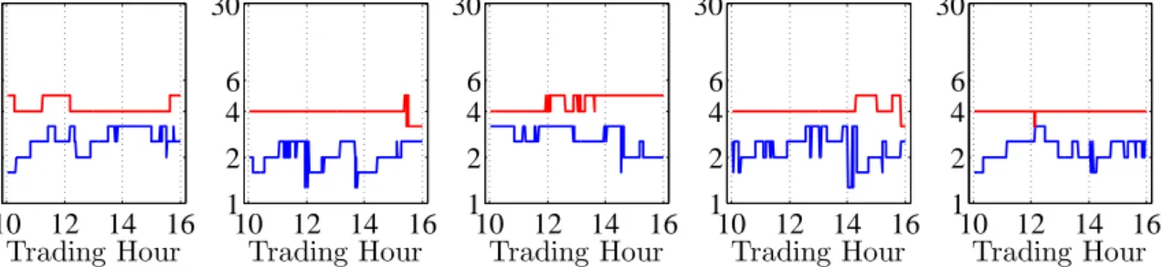
For illustration, the resulting adaptive choice of intervals at each minute on 2 February 2002 is shown by Figure 5. Adopting the EACD specification (for ρ= 0.25 and K = 13) in the modest risk case (r= 0.5, blue curve), one would select the length of the adaptive estimation interval lying between 1.5 and 3.5 hours over the course of the selected day. Likewise, in the conservative risk case (r = 1, red curve), the approach would select

10 12 14 16 1 2 4 6 30 AAPL Trading Hour Length in Hours 10 12 14 16 1 2 4 6 30 CSCO Trading Hour 10 12 14 16 1 2 4 6 30 INTC Trading Hour 10 12 14 16 1 2 4 6 30 MSFT Trading Hour 10 12 14 16 1 2 4 6 30 ORCL Trading Hour Figure 5: Estimated length of intervals of homogeneity n

b

k (in hours) for seasonally

ad-justed one-minute cumulative trading volumes of selected companies in case of a modest (r = 0.5, blue) and conservative (r = 1, red) modelling risk level. We use the interval scheme with K = 13 and ρ = 0.25. Underlying model: EACD(1,1). NASDAQ trading on 22 February 2008.

4.4

Empirical Findings

We apply the LPA to seasonally adjusted 1-min aggregated trading volumes for all five stocks at each minute from 22 February to 31 December 2008 (215 trading days, 77400 trading minutes). We use the EACD and WACD model as the two (local) specifications, two model risk levels (modest, r = 0.5, and conservative, r = 1) and two significance levels (ρ= 0.25 and ρ= 0.50). Furthermore, interval length schemes with (i)K = 8, and (ii) K = 13 are employed.

Figure 6 depicts the time series distributions of selected oracle interval lengths. Firstly, as expected, the chosen intervals are shorter in the modest risk case (r = 0.5) than in the conservative case (r = 1). Practically, if a trader aims at obtaining more precise volume estimates, it is advisable to select longer estimation periods, such as 4-5 hours. By doing so, the trader increases the modelling bias, but still can control it according to (8). Hence, this risk level allows for more controlled flexibility in modelling the data. Conversely, setting r = 1 implies a smaller modelling bias and thus lower estimation precision. Consequently, it yields smaller local intervals ranging between 2-3 hours in most cases.

window in practice. Interestingly, the procedure never selects the longest possible interval according to our interval scheme (one week of data), but chooses a maximum length of 6 hours. This finding suggests that even a week of data is clearly too long to capture parameter inhomogeneity in high-frequency variables. As a rough rule of thumb, a horizon of up to one trading day seems to be reasonable. This result is remarkably robust across the individual stocks suggesting that the stochastic properties of high-frequency trading volumes are quite similar, at least across (heavily traded) blue chips stocks. Nevertheless, as also illustrated in Figure 5, our findings show that the selected interval lengths clearly vary across time. Hence, a priori fixing the length of a rolling window can be still problematic and sub-optimal – even over the course of a day.

Thirdly, the optimal length of local windows does obviously also depend on the complexity of the underlying (local) model. In fact, we observe that local EACD specifications seem to sufficiently approximate the data over longer estimation windows than in case of WACD specifications. This is true for nearly all stocks and is most likely due to the variability of the Weibull shape parameter resulting in shorter intervals. Fourth, in Figure 7, we show time series averages of selected interval lengths in dependence of the time of the day. Even after removing the intraday seasonality component, we observe slightly shorter intervals in the opening and before closure. This is obviously induced by the fact that the local estimation window during the morning still includes significant information from the previous day. This effect is strongest at the opening where estimates are naturally based on previous day information solely and becomes weaker as time moves on and the fraction of current-day-information is increasing. Consequently, we observe the longest intervals around mid-day where most information in the local window stems from the current day. Hence, the LPA automatically accounts for the effects arising from concatenated time series omitting non-trading periods. During the afternoon, interval lengths further shrink as trading becomes more active (and obviously less time-homogeneous) before closure.

2h 4h 6h 0 0.5 1 AAPL Length Frequency 2h 4h 6h 0 0.5 1 CSCO Length 2h 4h 6h 0 0.5 1 INTC Length 2h 4h 6h 0 0.5 1 MSFT Length 2h 4h 6h 0 0.5 1 ORCL Length 2h 4h 6h 0 0.5 1 AAPL Length Frequency 2h 4h 6h 0 0.5 1 CSCO Length 2h 4h 6h 0 0.5 1 INTC Length 2h 4h 6h 0 0.5 1 MSFT Length 2h 4h 6h 0 0.5 1 ORCL Length

Figure 6: Distribution of estimated interval length n

bk

(in hours) for seasonally adjusted trading volumes of selected companies in case of modest (r = 0.5, red) and conservative modelling risk (r = 1, blue), using an EACD (upper panel) and a WACD model (lower panel) from 22 February to 31 December 2008 (215 trading days). We select 13 estimation windows based on significance level ρ= 0.25.

10 12 14 16 2h 2.5h 3h AAPL Trading Hour Length 10 12 14 16 2h 2.5h 3h CSCO Trading Hour 10 12 14 16 2h 2.5h 3h INTC Trading Hour 10 12 14 16 2h 2.5h 3h MSFT Trading Hour 10 12 14 16 2h 2.5h 3h ORCL Trading Hour 10 12 14 16 3.5h 4h 4.5h AAPL Trading Hour Length 10 12 14 16 3.5h 4h 4.5h CSCO Trading Hour 10 12 14 16 3.5h 4h 4.5h INTC Trading Hour 10 12 14 16 3.5h 4h 4.5h MSFT Trading Hour 10 12 14 16 3.5h 4h 4.5h ORCL Trading Hour

Figure 7: Average estimated interval lengthn

bk (in hours) over the course of a trading day

for seasonally adjusted trading volumes of selected companies in case of modest (r= 0.5, red) and conservative modelling risk (r = 1, blue), using an EACD (upper panel) and a WACD model (lower panel) from 22 February to 31 December 2008 (215 trading days). We select 13 based on significance level ρ= 0.25.

5

Forecasting Trading Volumes

Besides providing empirical evidence on the time (in)homogeneity of high-frequency data, our aim is to analyze the potential of the LPA when it comes to out-of-sample forecasts. The most important question is whether the proposed adaptive approach yields better predictions than a (rolling window) approach where the length of the estimation win-dow is fixed on an a priori basis. To set up the forecasting framework as realistic as possible, at each trading minute from February 22, to December 22, 2008, we predict the trading volume over all horizons h = 1,2, . . . ,60 min during the next hour. The predictions are computed using multi-step-ahead forecasts using the currently prevailing MEM parameters and initialized based on the data from the current local window. The local window is selected according to the LPA approach using r ∈ {0.5,1} and ρ ∈ {0.25,0.5}. Denoting the correspondingh-step prediction byybi+h, the resulting prediction

error isεbi+h = ˘yi+h−ybi+h, with ˘yi+h denoting the observed trading volume. As competing

approach, we consider predictions based on a fixed estimation window covering one day (i.e., 360 observations) and, alternatively, one week (i.e., 1800 observations) yielding predictionsyei+h and prediction errorsεei+h = ˘yi+h−yei+h. To account for the multiplicative

impact of intraday periodicities according to (1), we multiply the corresponding forecasts by the estimated seasonality component associated with the previous 30 days.

To test for the significance of forecasting superiority, we apply the Diebold and Mar-iano (1995) test. Define the loss differential dh between the squared prediction errors

stemming from both methods given horizonhand nobservations asdh ={di+h}n_i=1, with

di+h =εb

2

i+h−εe

2

i+h. Then, testing whether one forecasting model yields qualitatively lower

prediction errors is performed based on the statistic

TST,h = ( _n X i=1 I(di+h >0)−0.5n ) /√0.25n, (15)

test the null hypothesis H0 :E[dh] = 0 using the test statistic TDM,h = ¯dh/ q 2πfb_d h(0)/n L → N(0,1). (16)

Here, ¯dh denotes the average loss differential ¯dh =n−1Pni=1di+handfb_d

h(0) is a consistent

estimate of the spectral density of the loss differential at frequency zero. As shown by Diebold and Mariano (1995), the latter can be computed by

b fdh(0) = (2π) −1 hX−1 m=−(h−1) b γdh(m), (17) b γdh(m) =n −1 n X i=|m|+1 di+h−d¯h di+h−|m|−d¯h . (18)

Figure 8 displays the Diebold-Mariano test statisticsTDM,h against the forecasting horizon

h. The underlying LPA is based on the EACD model with significance level ρ = 0.25. Negative statistics indicate that the LPA provides smaller forecasting errors. We observe that in all cases, the fixed-window based forecast is worse than the LPA. The fixed-window approach performs particularly poorly if it utilizes windows covering one week of data. Hence, these windows seem to be clearly too long to cover local variations in parameters and thus yield estimates which are too strongly smoothed. Our results show that these misspecifications of (local) dynamics result in qualitatively significantly worse predictions. Conversely, fixed windows of one day seem to be much more appropriate resulting in clearly reduced (in absolute terms) statistics. Nevertheless, even in this context, the LPA significantly outperforms the fixed-window setting reflecting the importance of time-varying window lengths.

Analyzing the prediction performance in dependence of the forecasting horizon we observe that LPA-based predictions are particularly powerful over short horizons. The highest LPA overperformance is achieved at horizons of approximately 3-4 minutes. This is not surprising as the local adaptive estimates and thus corresponding forecasts are most appropriate in periods close to the local interval. Conversely, over longer prediction

horizons, the advantage of local modelling vanishes as the occurrence of further break points is more likely. We show that the best forecasting accuracy is achieved over horizons of up to 20 minutes. Finally, an important result is that the results are quite robust with respect to the choice of the modelling risk levelr. This makes the method quite universal and not critically dependent on the selection of steering parameters.

20 40 60 −40 −20 0 AAPL Test Statistic 20 40 60 −40 −20 0 Horizon Test Statistic 20 40 60 −40 −20 0 CSCO 20 40 60 −40 −20 0 Horizon 20 40 60 −40 −20 0 INTC 20 40 60 −40 −20 0 Horizon 20 40 60 −40 −20 0 MSFT 20 40 60 −40 −20 0 Horizon 20 40 60 −40 −20 0 ORCL 20 40 60 −40 −20 0 Horizon

Figure 8: Test statistic TDM,h across all 60 forecasting horizons for five large companies

traded at NASDAQ from 22 February to 22 December 2008 (210 trading days). The red curve depicts the statistic based on a test of the LPA against a fixed-window scheme using 360 observations (6 trading hours). The blue curve depicts the statistic based on a test of the LPA against a fixed-window scheme using 1800 observations (30 trading hours). The upper panel shows the results for the ’modest risk case’ (r = 0.5) and the lower panel shows the results for the ’conservative risk case’ (r= 1) given a significance level of ρ= 0.25.

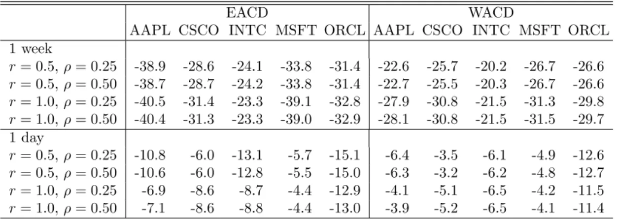
Table 4 summarizes test statistics TST,h. The table reports the correspondingly largest

(i.e., least negative) statistics across all 60 forecasting horizons. These results clearly con-firm the findings reported in Figure 8: The LPA produces significantly smaller (squared) forecasting errors in all cases. Moreover, Table 4 confirms the findings above that the forecasting accuracy is widely unaffected by the selection of LPA tuning parameters.

By depicting the ratio of root mean squared errors

v u u n−1 n X ε2 ,v_u u n−1 n X ε2 ,

Mar Jun Sep Dec 0.6

0.8 1

1.2 AAPL

Mar Jun Sep Dec 0.6

0.8 1

1.2 CSCO

Mar Jun Sep Dec 0.6

0.8 1

1.2 INTC

Mar Jan Sep Dec 0.6

0.8 1

1.2 MSFT

Mar Jun Sep Dec 0.6

0.8 1

1.2 ORCL

Mar Jun Sep Dec 0.6

0.8 1 1.2

Mar Jun Sep Dec 0.6

0.8 1 1.2

Mar Jun Sep Dec 0.6

0.8 1 1.2

Mar Jan Sep Dec 0.6

0.8 1 1.2

Mar Jun Sep Dec 0.6

0.8 1 1.2

Figure 9: Ratio between the RMSPEs of the LPA and of a fixed-window approach (cover-ing 6 trad(cover-ing hours) over the sample from 22 February to 22 December 2010 (210 trad(cover-ing days). Upper panel: Results for underlying (local) EACD model. Lower panel: Results for underlying (local) WACD model.

2 4 6 8 10 1 0.98 0.96 0.94 AAPL 2 4 6 8 10 0.94 0.96 0.98 1 CSCO 2 4 6 8 10 0.94 0.96 0.98 1 INTC 2 4 6 8 10 0.94 0.96 0.98 1 MSFT 2 4 6 8 10 0.94 0.96 0.98 1 ORCL 2 4 6 8 10 0.92 0.98 0.96 0.94 Horizon 2 4 6 8 10 0.94 0.96 0.98 1 Horizon 2 4 6 8 10 0.94 0.96 0.98 1 Horizon 2 4 6 8 10 0.94 0.96 0.98 1 Horizon 2 4 6 8 10 0.94 0.96 0.98 1 Horizon Figure 10: Ratio between the RMSPEs of the LPA and of a fixed-window approach (covering 6 trading hours) over the sample from 22 February to 22 December 2010 (210 trading days). Upper panel: EACD model, lower panel: WACD model.

EACD WACD

AAPL CSCO INTC MSFT ORCL AAPL CSCO INTC MSFT ORCL 1 week r= 0.5,ρ= 0.25 -38.9 -28.6 -24.1 -33.8 -31.4 -22.6 -25.7 -20.2 -26.7 -26.6 r= 0.5,ρ= 0.50 -38.7 -28.7 -24.2 -33.8 -31.4 -22.7 -25.5 -20.3 -26.7 -26.6 r= 1.0,ρ= 0.25 -40.5 -31.4 -23.3 -39.1 -32.8 -27.9 -30.8 -21.5 -31.3 -29.8 r= 1.0,ρ= 0.50 -40.4 -31.3 -23.3 -39.0 -32.9 -28.1 -30.8 -21.5 -31.5 -29.7 1 day r= 0.5,ρ= 0.25 -10.8 -6.0 -13.1 -5.7 -15.1 -6.4 -3.5 -6.1 -4.9 -12.6 r= 0.5,ρ= 0.50 -10.6 -6.0 -12.8 -5.5 -15.0 -6.3 -3.2 -6.2 -4.8 -12.7 r= 1.0,ρ= 0.25 -6.9 -8.6 -8.7 -4.4 -12.9 -4.1 -5.1 -6.5 -4.2 -11.5 r= 1.0,ρ= 0.50 -7.1 -8.6 -8.8 -4.4 -13.0 -3.9 -5.2 -6.5 -4.1 -11.4

Table 4: Largest (in absolute terms) test statistic TST,h across all 60 forecasting horizons

as well as EACD and WACD specifications for five large companies traded at NASDAQ from 22 February to 22 December 2008 (210 trading days). We compare LPA-implied forecasts with those based on rolling windows using a priori fixed lengths of one week and one day, respectively. Negative values indicate lower squared prediction errors resulting from the LPA. According to the Diebold-Mariano test (16), the average loss differential is significantly negative in all cases (significance level 5%).

Figure 9 provides deeper insights into the forecasting performance of the two competing approaches over time and over the sample. In most cases, the ratio is clearly below one and thus also indicates a better forecasting performance of the LPA method. This is particularly true during the last months and thus the height of the financial crisis in 2008. During this period, market uncertainty has been high and trading activity has been subject to various information shocks. Our results show that the flexibility offered by the LPA is particularly beneficial in such periods whereas fixed-window approaches tend to perform poorly. Similar results are reported in the context of daily volatility modelling during periods of financial distress, see Čížek et al. (2009). Moreover, it turns out that the results do not critically depend on the choice of the underlying local model as the findings based on EACD and WACD models are quite comparable.

Figure 10 shows the ratio of root mean squared errors in dependence of the length of the forecasting horizon (in minutes). It turns out that the LPA’s overperformance is strongest over horizons between two and four minutes. Over these intervals, the effects of superior (local) estimates of MEM parameters fully pay out. Over longer horizons, differences in

prediction performance naturally shrink as forecasts converge to unconditional averages.

6

Conclusions

We propose a local adaptive multiplicative error model (MEM) for financial high-frequency variables. The approach addresses the inherent inhomogeneity of parameters over time and is based on local window estimates of MEM parameters. Adapting the local paramet-ric approach (LPA) by Spokoiny (1998) and Mercurio and Spokoiny (2004), the length of local estimation intervals is chosen by a sequential testing procedure. Balancing mod-elling bias and estimation (in)efficiency, the approach provides the longest interval of parameter homogeneity which is used to (locally) estimate the model and to compute corresponding forecasts.

Applying the proposed approach to the high-frequency series of one-minute cumulative trading volumes based on several NASDAQ blue chip stocks, we can conclude as follows: First, MEM parameters reveal substantial variations over time. Second, the optimal length of local intervals varies between one and six hours. Nevertheless, as a rule of thumb, local intervals of around four hours are suggested. Third, the local adaptive approach provides significantly better out-of-sample forecasts than competing approaches using a priori fixed lengths of estimation intervals. This result demonstrates the importance of an adaptive approach. Finally, we show that the findings are robust with respect to the choice of LPA steering parameters controlling modelling risk.

As the stochastic properties of cumulative trading volumes are similar to those of other (persistent) high-frequency series, our findings are likely to be carried over to, for instance, the time between trades, trade counts, volatilities, bid-ask spreads and market depth. Hence, we conclude that adaptive techniques constitute a powerful device to improve high-frequency forecasts and to gain deeper insights into local variations in model parameters and thus structural relationships.

References

Brownlees, C. T., Cipollini, F. and Gallo, G. M. (2011). Intra-daily Volume Modeling and Prediction for Algorithmic Trading,Journal of Financial Econometrics 9(3): 489–518. Chen, Y., Härdle, W. and Pigorsch, U. (2010). Localized Realized Volatility, Journal of

the American Statistical Association105(492): 1376–1393.

Čížek, P., Härdle, W. K. and Spokoiny, V. (2009). Adaptive pointwise estimation in time-inhomogeneous conditional heteroscedasticity models, Econometrics Journal 12: 248– 271.

Diebold, F. and Mariano, R. S. (1995). Comparing Predictive Accuracy, Journal of Business and Economic Statistics 13(3): 253–263.

Engle, R. F. (1982). Autoregressive Conditional Heteroscedasticity with Estimates of the Variance of United Kingdom Inflation,Econometrica 50(4): 987–1007.

Engle, R. F. (2002). New Frontiers for ARCH Models, Journal of Applied Econometrics

17: 425–446.

Engle, R. F. and Rangel, J. G. (2008). The Spline-GARCH Model for Low-Frequency Volatility and Its Global Macroeconomic Causes,Review of Financial Studies21: 1187– 1222.

Engle, R. F. and Russell, J. R. (1998). Autoregressive Conditional Duration: A New Model for Irregularly Spaced Transaction Data,Econometrica 66(5): 1127–1162. Gallant, A. R. (1981). On the bias of flexible functional forms and an essentially unbiased

form, Journal of Econometrics 15: 211–245.

Hautsch, N. (2012). Econometrics of Financial High-Frequency Data, Springer, Berlin. Hautsch, N., Malec, P. and Schienle, M. (2011). Capturing the Zero: A New Class of

Hujer, R., Vuletić, S. and Kokot, S. (2002). The Markov Switching ACD Model,Working paper - finance and accounting, no. 90, Johann Wolfgang Goethe-University Frankfurt. Manganelli, S. (2005). Duration, volume and volatility impact of trades, Journal of

Financial Markets8: 377–399.

Meitz, M. and Teräsvirta, T. (2006). Evaluating Models of Autoregressive Conditional Duration,Journal of Business and Economic Statistics 24(1): 104–124.

Mercurio, D. and Spokoiny, V. (2004). Statistical inference for time-inhomogeneous volatility models, The Annals of Statistics32(2): 577–602.

Spokoiny, V. (1998). Estimation of a function with discontinuities via local polynomial fit with an adaptive window choice, The Annals of Statistics26(4): 1356–1378.

Spokoiny, V. (2009). Multiscale local change point detection with applications to Value-at-Risk, The Annals of Statistics37(3): 1405–1436.

Tong, H. (1990). Non-linear Time Series: A Dynamical System Approach, Oxford Uni-versity Press, Oxford.

Zhang, M. Y., Russell, J. R. and Tsay, R. S. (2001). A nonlinear autoregressive conditional duration model with applications to financial transaction data,Journal of Econometrics

SFB 649 Discussion Paper Series 2012

For a complete list of Discussion Papers published by the SFB 649, please visit http://sfb649.wiwi.hu-berlin.de.

SFB 649, Spandauer Straße 1, D-10178 Berlin

001 "HMM in dynamic HAC models" by Wolfgang Karl Härdle, Ostap Okhrin and Weining Wang, January 2012.

002 "Dynamic Activity Analysis Model Based Win-Win Development Forecasting Under the Environmental Regulation in China" by Shiyi Chen and Wolfgang Karl Härdle, January 2012.

003 "A Donsker Theorem for Lévy Measures" by Richard Nickl and Markus Reiß, January 2012.

004 "Computational Statistics (Journal)" by Wolfgang Karl Härdle, Yuichi Mori

and Jürgen Symanzik, January 2012.

005 "Implementing quotas in university admissions: An experimental analysis" by Sebastian Braun, Nadja Dwenger, Dorothea Kübler and Alexander Westkamp, January 2012.

006 "Quantile Regression in Risk Calibration" by Shih-Kang Chao, Wolfgang Karl Härdle and Weining Wang, January 2012.

007 "Total Work and Gender: Facts and Possible Explanations" by Michael Burda, Daniel S. Hamermesh and Philippe Weil, February 2012.

008 "Does Basel II Pillar 3 Risk Exposure Data help to Identify Risky Banks?"

by Ralf Sabiwalsky, February 2012.

009 "Comparability Effects of Mandatory IFRS Adoption" by Stefano Cascino and Joachim Gassen, February 2012.

010 "Fair Value Reclassifications of Financial Assets during the Financial Crisis" by Jannis Bischof, Ulf Brüggemann and Holger Daske, February 2012.

011 "Intended and unintended consequences of mandatory IFRS adoption: A

review of extant evidence and suggestions for future research" by Ulf Brüggemann, Jörg-Markus Hitz and Thorsten Sellhorn, February 2012. 012 "Confidence sets in nonparametric calibration of exponential Lévy

models" by Jakob Söhl, February 2012.

013 "The Polarization of Employment in German Local Labor Markets" by Charlotte Senftleben and Hanna Wielandt, February 2012.

014 "On the Dark Side of the Market: Identifying and Analyzing Hidden Order

Placements" by Nikolaus Hautsch and Ruihong Huang, February 2012.

015 "Existence and Uniqueness of Perturbation Solutions to DSGE Models" by

Hong Lan and Alexander Meyer-Gohde, February 2012.

016 "Nonparametric adaptive estimation of linear functionals for low frequency observed Lévy processes" by Johanna Kappus, February 2012. 017 "Option calibration of exponential Lévy models: Implementation and

empirical results" by Jakob Söhl und Mathias Trabs, February 2012. 018 "Managerial Overconfidence and Corporate Risk Management" by Tim R.

Adam, Chitru S. Fernando and Evgenia Golubeva, February 2012.

019 "Why Do Firms Engage in Selective Hedging?" by Tim R. Adam, Chitru S.

Fernando and Jesus M. Salas, February 2012.

020 "A Slab in the Face: Building Quality and Neighborhood Effects" by Rainer Schulz and Martin Wersing, February 2012.

021 "A Strategy Perspective on the Performance Relevance of the CFO" by Andreas Venus and Andreas Engelen, February 2012.

022 "Assessing the Anchoring of Inflation Expectations" by Till Strohsal and Lars Winkelmann, February 2012.

SFB 649 Discussion Paper Series 2012

For a complete list of Discussion Papers published by the SFB 649, please visit http://sfb649.wiwi.hu-berlin.de.

023 "Hidden Liquidity: Determinants and Impact" by Gökhan Cebiroglu and Ulrich Horst, March 2012.

024 "Bye Bye, G.I. - The Impact of the U.S. Military Drawdown on Local German Labor Markets" by Jan Peter aus dem Moore and Alexandra Spitz-Oener, March 2012.

025 "Is socially responsible investing just screening? Evidence from mutual

funds" by Markus Hirschberger, Ralph E. Steuer, Sebastian Utz and Maximilian Wimmer, March 2012.

026 "Explaining regional unemployment differences in Germany: a spatial panel data analysis" by Franziska Lottmann, March 2012.

027 "Forecast based Pricing of Weather Derivatives" by Wolfgang Karl Härdle, Brenda López-Cabrera and Matthias Ritter, March 2012.

028 “Does umbrella branding really work? Investigating cross-category brand

loyalty” by Nadja Silberhorn and Lutz Hildebrandt, April 2012.

029 “Statistical Modelling of Temperature Risk” by Zografia Anastasiadou,

and Brenda López-Cabrera, April 2012.

030 “Support Vector Machines with Evolutionary Feature Selection for Default

Prediction” by Wolfgang Karl Härdle, Dedy Dwi Prastyo and Christian Hafner, April 2012.

031 “Local Adaptive Multiplicative Error Models for High-Frequency

Forecasts” by Wolfgang Karl Härdle, Nikolaus Hautsch and Andrija Mihoci, April 2012.

SFB 649, Spandauer Straße 1, D-10178 Berlin http://sfb649.wiwi.hu-berlin.de