K. C. Chambers , N. Kaiser , E. A. Magnier , P. A. Price , and J. L. Tonry 1Department of Astronomy, University of Maryland, College Park, MD 20742-2421, USA;[email protected]
2Astronomy Department, California Institute of Technology, MC 249-17, 1200 East California Boulevard, Pasadena, CA 91125, USA 3Institute for Astronomy, University of Hawaii, 2680 Woodlawn Drive, Honolulu, HI 96822, USA
4Department of Physics and Astronomy, Johns Hopkins University, 3400 North Charles Street, Baltimore, MD 21218, USA 5Laboratory for Astronomy and Solar Physics, NASA Goddard Space Flight Center, Greenbelt, MD 20771, USA
6Observatories of the Carnegie Institute of Washington, Pasadena, CA 90095, USA 7Department of Astronomy, Columbia University, New York, NY 10027, USA 8Department of Astrophysical Sciences, Princeton University, Princeton, NJ 08544, USA
Received 2012 November 19; accepted 2013 February 1; published 2013 March 7
ABSTRACT
We present the selection and classification of over a thousand ultraviolet (UV) variable sources discovered in
∼40 deg2ofGALEXTime Domain Survey (TDS) NUV images observed with a cadence of 2 days and a baseline
of observations of∼3 years. TheGALEXTDS fields were designed to be in spatial and temporal coordination with the Pan-STARRS1 Medium Deep Survey, which provides deep optical imaging and simultaneous optical transient detections via image differencing. We characterize theGALEXphotometric errors empirically as a function of mean magnitude, and select sources that vary at the 5σ level in at least one epoch. We measure the statistical properties of the UV variability, including the structure function on timescales of days and years. We report classifications for theGALEXTDS sample using a combination of optical host colors and morphology, UV light curve characteristics, and matches to archival X-ray, and spectroscopy catalogs. We classify 62% of the sources as active galaxies (358 quasars and 305 active galactic nuclei), and 10% as variable stars (including 37 RR Lyrae, 53 M dwarf flare stars, and 2 cataclysmic variables). We detect a large-amplitude tail in the UV variability distribution for M-dwarf flare stars and RR Lyrae, reaching up to|Δm| =4.6 mag and 2.9 mag, respectively. The mean amplitude of the structure function for quasars on year timescales is five times larger than observed at optical wavelengths. The remaining unclassified sources include UV-bright extragalactic transients, two of which have been spectroscopically confirmed to be a young core-collapse supernova and a flare from the tidal disruption of a star by dormant supermassive black hole. We calculate a surface density for variable sources in the UV with NUV <23 mag and|Δm|>0.2 mag of
∼8.0, 7.7, and 1.8 deg−2for quasars, active galactic nuclei, and RR Lyrae stars, respectively. We also calculate a
surface density rate in the UV for transient sources, using the effective survey time at the cadence appropriate to each class, of∼15 and 52 deg−2yr−1for M dwarfs and extragalactic transients, respectively.
Key words: surveys – ultraviolet: general
Online-only material:color figures, machine-readable table
1. INTRODUCTION
Unlike the optical, X-ray, and γ-ray sky, which have been systematically studied in the time domain in the search for supernovae (SNe) and gamma-ray bursts (GRBs), the wide-field ultraviolet (UV) time domain is a relatively unexplored parameter space. The launch of theGALEXsatellite with its 1◦.25 diameter field of view, and limiting sensitivity per 1.5 ks visit of
∼23 mag in the FUV (λeff=1539 Å) and NUV (λeff =2316 Å;
Martin et al.2005; Morrissey et al.2007), enabled the discovery of UV variable sources in repeated observations over hundreds of square degrees for the first time.
The UV waveband is particularly sensitive to hot (≈104K)
thermal emission from such transient and variable phenomena as young core-collapse SNe, the inner regions of the accretion flow around accreting supermassive black holes (SMBHs), and the flaring states of variable stars. The characteristic timescales of variables and transients in the UV range from minutes to years. M dwarf flare stars have strong magnetic activity that manifests itself in flares of thermal UV emission on the timescale of minutes (Kowalski et al.2009). RR Lyrae stars have periodic
pulsations which drive temperature fluctuations from∼6000 to 8000 K that cause periodic variability in the UV on a timescale of ∼0.5 d (Wheatley et al. 2012). Core-collapse SNe remain bright in the UV for hours up to several days following shock breakout, depending on the radius of the progenitor star (Nakar & Sari 2010; Rabinak & Waxman 2011), and the presence of a dense wind (Ofek et al. 2010; Chevalier & Irwin 2011; Svirski et al.2012). Active galactic nuclei (AGNs) and quasars demonstrate stronger variability with decreasing wavelength and longer timescales of years (Vanden Berk et al.2004).
UV variability studies of GALEX data observed as part of the All-Sky, Medium, and Deep Imaging baseline mission surveys (AIS, MIS, DIS) from 2003 to 2007, yielded the detection of M-dwarf flare stars (Welsh et al.2007), RR Lyrae stars, AGN, and quasars (Welsh et al. 2005, 2011; Wheatley et al. 2008), and flares from the tidal disruption of stars around dormant SMBHs (Gezari et al. 2006, 2008a, 2009). Serendipitous overlap of fourGALEXDIS fields with the optical Canada–France–Hawaii Telescope (CFHT) Supernova Legacy Survey, enabled the extraction of simultaneous optical light curves from image differencing for two of the tidal disruption
dense circumstellar medium (Ofek et al.2010).
Motivated by the promising results from the analysis of random repeatedGALEX observations, and the demonstrated value of overlap with optical time domain surveys, we initiated a dedicatedGALEXTime Domain Survey (TDS) to systematically study UV variability on timescales of days to years with multiple epochs of NUV images observed with a regular cadence of 2 days. TheGALEXTDS fields were selected to overlap with the Pan-STARRS1 Medium Deep Survey (PS1 MDS; Kaiser et al.
2010).GALEXTDS and PS1 MDS are well matched in field of view, sensitivity, and cadence (shown in Table1). Here we present the analysis of 42GALEXTDS fields which intersect with the PS1 MDS footprint, for a total area on the sky of 39.91 deg2, which were monitored over a baseline of 3.32 years (2008 February–2011 June). In this paper we use PS1 MDS deep stack catalogs to characterize the optical hosts ofGALEXTDS sources. Simultaneous UV and optical variability of GALEX TDS sources culled from matches with the PS1 transient alerts (Huber et al.2011) will be presented in future papers.
The paper is structured as follows. In Section2we describe theGALEXTDS survey design, and in Section3we describe our statistical methods for selecting UV-variable sources and characterizing their UV variability. In Section 4 we describe the multiwavelength catalog data used to identify the hosts of the UV-variable sources, including archival optical data, a deep PS1 MDS catalog, and archival redshift and X-ray catalogs. In Section 5 we describe our sequence of steps for classifying the GALEX TDS sources, in Section 6 we summarize our classification results, and the UV variability properties of our classified sources. In Section7we conclude with implications for future surveys.
2.GALEXTDS OBSERVATIONS
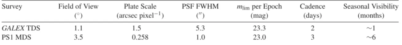
GALEXTDS monitored 6 out of 10 total PS1 MDS fields, with 7GALEXTDS pointings (labeled PS_fieldname_MOSpointing) at a time to cover the PS1 7 deg2field of view. During the window
of observing visibility of eachGALEXTDS field (from two to four weeks, one to two times per year), they were observed with a cadence of 2 days, and a typical exposure time per epoch of 1.5 ks (or a 5σ point-source limit of mAB ∼ 23.3 mag),
with a range from 1.0 to 1.7 ks. The NUV detector developed a problem on 2010 May 4 during observations of PS_ELAISN1, and so we do not include epochs observed between this time and when the instrument was fixed on 2010 June 23 in our analysis. Figure1shows the position of theGALEXTDS fields relative to the PS1 MDS fields, and Table2lists the R.A. and decl. of their centers, the Galactic extinction (E(B −V)) for each field from the Schlegel et al. (1998) dust maps, and the
PS_XMMLSS_MOS03 35.875 −4.250 0.026 27 PS_XMMLSS_MOS04 36.900 −4.420 0.026 27 PS_XMMLSS_MOS05 35.200 −5.050 0.022 26 PS_XMMLSS_MOS06 36.230 −5.200 0.027 24 PS_CDFS_MOS00 53.100 −27.800 0.008 114 PS_CDFS_MOS01 52.012 −28.212 0.008 30 PS_CDFS_MOS02 53.124 −26.802 0.009 29 PS_CDFS_MOS03 54.165 −27.312 0.012 30 PS_CDFS_MOS04 52.910 −28.800 0.009 30 PS_CDFS_MOS05 52.111 −27.276 0.010 30 PS_CDFS_MOS06 53.970 −28.334 0.010 6 PS_COSMOS_MOS21 150.500 +3.100 0.023 15 PS_COSMOS_MOS22 149.500 +3.100 0.027 16 PS_COSMOS_MOS23 151.000 +2.200 0.024 24 PS_COSMOS_MOS24 150.000 +2.200 0.020 26 PS_COSMOS_MOS25 149.000 +2.300 0.023 13 PS_COSMOS_MOS26 150.500 +1.300 0.023 26 PS_COSMOS_MOS27 149.500 +1.300 0.019 27 PS_GROTH_MOS01 215.600 +54.270 0.011 17 PS_GROTH_MOS02 213.780 +54.350 0.015 16 PS_GROTH_MOS03 214.146 +53.417 0.009 17 PS_GROTH_MOS04 212.400 +53.700 0.011 18 PS_GROTH_MOS05 215.500 +52.770 0.008 19 PS_GROTH_MOS06 214.300 +52.550 0.008 8 PS_GROTH_MOS07 212.630 +52.750 0.009 19 PS_ELAISN1_MOS10 242.510 +55.980 0.007 17 PS_ELAISN1_MOS11 244.570 +55.180 0.009 17 PS_ELAISN1_MOS12 242.900 +55.000 0.008 18 PS_ELAISN1_MOS13 241.300 +55.350 0.007 18 PS_ELAISN1_MOS14 243.960 +54.200 0.010 19 PS_ELAISN1_MOS15 242.400 +54.000 0.011 21 PS_ELAISN1_MOS16 241.380 +54.450 0.010 19 PS_VVDS22H_MOS00 333.700 +1.250 0.040 39 PS_VVDS22H_MOS01 332.700 +0.700 0.046 35 PS_VVDS22H_MOS02 334.428 +0.670 0.057 38 PS_VVDS22H_MOS03 333.600 +0.200 0.058 27 PS_VVDS22H_MOS04 334.610 −0.040 0.093 24 PS_VVDS22H_MOS05 333.900 −0.720 0.102 35 PS_VVDS22H_MOS06 332.900 −0.400 0.113 33
number of epochs per field. The median number of epochs per field is 24. PS_CDFS_MOS00 is an exception with 114 epochs, because it was monitored with a rapid cadence (|Δt| ∼ 3 hr) over a period of 10 days in 2010 November. Some offsets in the GALEXpointings from the footprint of the PS1 MDS fields were necessary in order to avoid UV-bright stars in the field of view that would violate the detector’s bright-source count limits.
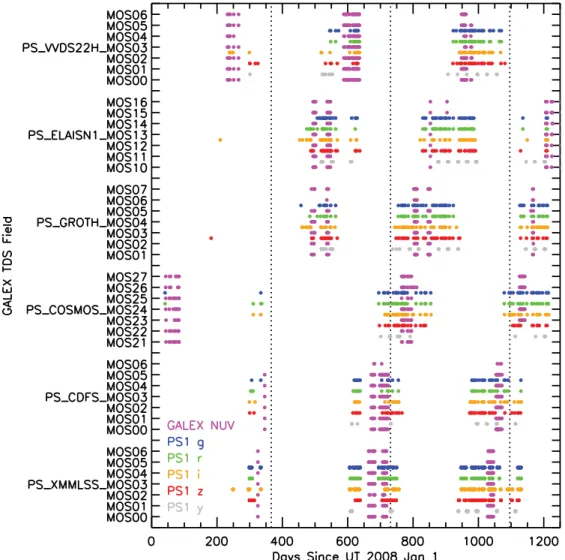
Figure 2 shows the temporal sampling of GALEX TDS observations in the NUV in comparison to the PS1 MDS observations in thegP1,rP1,iP1,zP1, andyP1 bands from 2008
Figure 1.GALEXTDS 1.◦1 diameter field pointings shown in blue, and the PS1 MDS 3◦.5 diameter field pointings shown in green. Orange hatched regions show the coverage of SDSS in the optical, red hatched regions shows the coverage of SWIRE in the optical, and cyan rectangles indicate the coverage of the CFHTLS Deep (solid lines) and Wide (dashed lines) surveys in the optical. Light gray regions show the coverage ofXMM-NewtonX-ray observations, and dark gray regions show the coverage ofChandraX-ray observations.
(A color version of this figure is available in the online journal.)
February to 2011 June. PS1 began taking commissioning data of the MDS fields in 2009 May, but did not begin full survey operations until a year later. TheGALEXfar-UV (FUV) detector became non-operational in 2009 May, and so we only include near-UV (NUV) images in our study.
3. STATISTICAL MEASUREMENTS 3.1. Selection of Variable Sources
Since most galaxies are unresolved by the GALEX NUV 5.3 FWHM point-spread function (PSF), we can use simple aperture photometry instead of image differencing to measure variability. We create a master list of unique source positions from the pipeline-generated catalogs (Morrissey et al. 2007) for all the individual epochs, as well as deep stacks of all the epochs, using a clustering radius of 5. This radius is chosen such that for the typical astrometry error of GALEX of 0.5, the Bayesian probability that the match is real is larger than the Bayesian probability that the match is spurious (Budav´ari & Szalay2008). The final master list includes 419,152 sources.
In order to select intrinsically variable sources in our survey, we first need to characterize the photometric errors. Although theGALEXimages are Poisson-limited, the Poisson error un-derestimates the total error in theGALEXcatalog magnitudes by a factor of ∼2 (Trammell et al. 2007). This discrepancy is attributed to systematic errors such as uncertainties in the
detector background and flat-field. Thus, we measure the pho-tometric errorempiricallyby calculating the standard deviation of aperture magnitudes in bins of mean magnitude, m. We only include objects in the pipeline-generated catalogs that are detected in all or 10 epochs. In each bin of Nobjects with
mi =(
n
k=1mi,k)/n(each bin typically hasN=50 to 1000
sources), we calculate for each epochkof a total ofnepochs,
σ(m, k)= 1 N−1 N i=1 (mi,k− mi)2, (1)
where mi,k is the magnitude (in the AB system) given by
mi,k = −2.5 log(f6) +zp+ Cap −8.2E(B −V), f6 is the
background-subtracted flux in a 6radius aperture,zp=20.08, the aperture correction isCap = −0.23 mag (Morrissey et al.
2007), and we correct for Galactic extinction using the values forE(B−V) listed in Table2. We use 3σ clipping to remove outliers in the calculation of σ(m, k) which can arise from artifacts.
The astrometric precision depends on the signal-to-noise of the source, thus we also empirically measure a magnitude-dependent clustering radius. We do so by measuring the cu-mulative distribution of spatial separations between the position in each epoch and the mean position for sources in bins ofm, and recordd95(m, k), the value for which 95% of sources have
a separation less than or equal to that value. The resulting value ford95is a strong function magnitude, increasing from∼1for
Figure 2.Dates ofGALEXTDS NUV observations compared to PS1 MDS observations in thegP1,rP1,iP1,zP1, andyP1bands. Dotted lines show yearly intervals. (A color version of this figure is available in the online journal.)
m =18.0 mag to∼4form =23.0 mag. Figures3and4
showσ(m, k) andd95(m, k) for an example GALEX TDS
field PS_COSMOS_MOS23, a quadratic fit to the median func-tion for all epochs in that field, and the median funcfunc-tion fit over all fields.
In our master list of source positions, we include all sources detected, including sources detected in only one epoch, and fix the centroid to the epoch for which the source is detected with maximum flux. We measure forced aperture magnitudes at the positions of each source in epochs where the source was not detected by the pipeline or the spatial separation of the matched source is greater thand95(m, k). When the aperture magnitude
is fainter thanmlimin an epoch, it is flagged as an upper limit and
replaced withmlim, wheremlim= −2.5 log(5
(BskyNpix/Texp)+
zp+Cap, whereBsky=3×10⁻³counts s−1pixel−1,Npix=16π,
andTexpis the exposure time of that epoch in seconds.
We select sources that have at least one epoch for which
|mk− m|> 5σ(m, k), wherem is calculated only from
epochs that have a magnitude above the detection limit of that epoch. We use this selection method to be sensitive to short-term and long-term variability, as well as transients. This 5σ selection is quite conservative, and requires variability amplitudes increasing from|Δm|>0.1 mag form ∼18 mag up to|Δm|>1.0 mag form ∼23 mag.
Figure 3. Empirical determination of 1σ photometric errors as a function of mean magnitude from the standard deviation of sources detected by the pipeline catalogs in 10 epochs for one of the GALEX TDS fields PS_COSMOS_MOS23. Solid green line shows a quadratic fit to the error function for the field PS_COSMOS_MOS23, and dashed blue line shows a quadratic fit to the median error function for all of theGALEXTDS fields. Solid red line shows the expected 1σ Poisson error, which underestimates the total photometric error by a factor of∼2.
Figure 4.Maximum spatial separation from the mean for 95% of the sources as a function of mean magnitude from the cumulative distribution of sources detected by the pipeline catalogs in10 epochs for one of theGALEXTDS fields PS_COSMOS_MOS23. Solid green line shows a quadratic fit to the error function for the field PS_COSMOS_MOS23, and dashed blue line shows a quadratic fit to the median distance function for all of theGALEXTDS fields. Note that due to systematic differences in the PSF between fields, the distance function radius for PS_COSMOS_MOS23 is up to∼1smaller than the median for all fields, since form20 mag,d95∼2in the PS_XMMLSS, PS_CDFS, PS_GROTH, and PS_ELAISN1 fields andd95∼3in the PS_VVDS22H fields. (A color version of this figure is available in the online journal.)
We make the following cuts to the 5σvariable source sample to remove artifacts.
1. We remove sources with pipeline artifact flags indicating window bevel reflections or ghosts from the dichroic beam splitter.
2. We remove the brightest objects, with m < 18.0, due to the large area subtended by the PSF which causes uncertainty in the background subtraction.
3. We select sources within a radius of 0◦.55 of the center of the field, in order to avoid glints and PSF distortions, which are more prominent on the edges of the image, from un-corrected spatial distortions of photons recorded by the detectors.
4. We do not include objects that are within 1.5 of am <
17 mag source, to avoid regions affected by the bright source’s PSF and ghost artifacts. Ghost artifacts can appear within 30–60 above and below a bright source in the Y detector direction. Ghosts are point-like, and thus can only be identified from their Y detector position relative to a bright source. While ghosts do not usually appear in theGALEX pipeline catalogs, we apply this cut since our forced aperture photometry could mistake ghosts for transient sources.
5. We veto objects for which in the epoch of maximum
|mk− m|/σ(m, k) or maximum flux, the aperture flux
ratio of the object hasf6/f3.8 > R90, where f6 is the 6.0
radius aperture flux, f3.8 is the 3.8 radius aperture flux,
and R90 is the maximum cumulative aperture flux ratio
measured for 90% of the sources in the reference source sample used to calculateσ(m, k) in that epoch. This cut removes fluctuations in the background due to reflections from bright stars just outside the field-of-view, as well as epochs where the PSF is distorted due to a degradation in resolution which sometimes occurs in the Y detector direction. This also vetoes cases when the pipeline shreds
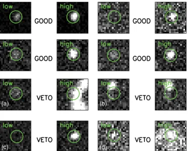
(a)
(c)
(b)
(d)
Figure 5.Left: gallery of good and vetoed variable sources during their epochs of minimum (“low”) and maximum (“high”) flux. The green circle shows a 6(4 pixel) aperture radius. Sources vetoed forf6/f3.8 > R90are shown in panels (a) and (b), a source vetoed as a likely ghost within 1.5 of am <17 mag source is shown in panel (c), and a manually vetoed source is shown in panel (d). For each source the gray scale is linear, and is scaled to the peak of the source in its “high” state.
(A color version of this figure is available in the online journal.)
a source into multiple sources, and the source is detected as variable because the center of the aperture is off-center from the peak source flux.
6. Finally, we visually inspect all of the remaining variable sources to remove any remaining artifacts that passed through the cuts above.
Figure5shows a gallery of good sources and vetoed variable sources from our automated cuts (for a bright reflection in panel (a), an off-center source in panel (b), and a likely ghost in panel (c)) and manual cuts (for a diffuse reflection in panel (d)). Our finalGALEXTDS 5σvariable sample after the cuts listed above has a total of 1078 sources.
3.2. Variability Statistics
We characterize the variability of each 5σvariable UV source using several statistical measures. We measure the structure function (following di Clemente et al. (1996)),
V(Δt)= π 2|Δmij| 2 Δt− σi2+σj2 Δt, (2)
where brackets denote averages for all pairs of points on the light curve of an individual source withi < jandtj −ti =Δt.
The two-day cadence of the observations combined with the seasonal visibility of the fields results in a distribution of time intervals between observations (shown in Figure6) that fall into six characteristic timescale bins: Δt2 d = 2±0.5 d,
Δt4 d = 4 ±0.5 d, Δt6 d = 6 ±0.5 d, Δt8 d = 8 ±0.5 d,
Δt1 yr = 0.96±0.14 yr, and Δt2 yr = 1.96±0.04 yr. We
measure the structure function in these six bins, and define Sdto be the maximum value of the structure function evaluated
forΔt2 d,Δt4 d,Δt6 d, andΔt8 d, andSyrto be the maximum value
of the structure function evaluated forΔt1 yrandΔt2 yr. We also
measure the intrinsic variability as defined by Sesar et al. (2007),
σint=
Σ2−ξ2, whereΣ2=(1/n−1)n
Figure 6.Histogram of the time intervals between all pairs of observations for the 42 fields inGALEXTDS. Hatched regions show the time intervals over which the structure function is measured for all of the sources.
ξ2 =(1/n)nk=1σ(m, k)2, and the maximum amplitude of
variability, max(|Δm|).
3.3. UV Light Curve
In order to flag possible transient UV events that may be associated with a SN or TDE, we differentiate between stochastic variability and flaring variability. We identify flaring UV variability as sources that show a constant flux10 days before the peak of the light curve, and do not fade more than 2σ below the faintest pre-peak magnitude (measured 10 days before the peak). This selection criteria is tailored to the NUV rise times observed in SNe (Gezari et al.2008b,
2010; Brown et al.2009; Milne et al.2010; Ofek et al.2010) and TDE candidates (Gezari et al. 2006, 2008a, 2009). We define constant pre-peak flux as a light curve with a reduced
χν2/ <3(χν2 =pk=1(mk− m)2/(σ(m, k)2/(n−1), where
nis the number of epochs10 days before the peak). For those sources for which there are only upper limits10 days before the peak, χν2 is set to 1. Flaring sources with no detections before the peak are further labeled as transients. Sources with
χν2/ 3, or that fade below 2σ of the faintest magnitude measured10 days before the peak are labeled as stochastically variable. We flag 116 flares, 145 transients, 595 stochastically variable sources, and remain with 222 sources with neither light-curve classification flag. In Figure7 we show example light curves of sources flagged as stochastically variable (“V”), flares (“F“), and transients (“T”).
4. HOST PROPERTIES 4.1. Archival Optical Imaging Catalogs
We first characterize the host properties of the UV variable sources using archival opticalu,g,r,i, andzphotometry and morphology from matches to the Sloan Digital Sky Survey (SDSS) Photometric Catalog, Release 8 (Aihara et al. 2011;
mlim ∼ 22 mag), the CFHTLS Deep Fields D1, D2, and D3
(mlim ∼26.5 mag) and Wide Fields W1, W3, and W4 (mlim ∼
25 mag) merged catalogs version T0005,9 and the SWIRE ELAIS N1 and CDFS Region catalogs (mlim∼24 mag; Surace
et al. 2004). For sources with matches in multiple catalogs,
9 http://terapix.iap.fr/rubrique.php?id_rubrique=252
Figure 7.Example light curves of sources flagged as stochastically variable (“V”), flares (“F”), and transient flares (“T”). Epochs10 days before the epoch of peak flux are circled in red, and the epoch of peak flux is circled in blue. The thick dashed line indicates the mean flux10 days before the peak. (A color version of this figure is available in the online journal.)
we use the match from the deepest catalog. We convert the CFHTLS magnitudes to the SDSS system using the conversions in Regnault et al. (2009), and the SWIRE Vega magnitudes to the SDSS system using the transformations measured for stellar objects available at the INT WFS Web site.10 We then correct for Galactic extinction using the Schlegel et al. (1998) dust map values forE(B−V) listed in Table2. Figure1shows the overlap of the GALEXTDS fields with the available archival optical catalogs.
4.2. Pan-STARRS1 Medium Deep Survey
The GALEX TDS fields overlap with the PS1 MDS fields MD01 (PS_XMMLSS), MD02 (PS_CDFS), MD04 (PS_COSMOS), MD07 (PS_GROTH), MD08 (PS_ELAISN1), and MD09 (PS_VVDS22H). The Pan-STARRS1 observations are obtained through a set of five broadband filters, (gP1,rP1,
iP1,zP1, andyP1). Further information on the passband shapes
is described in Stubbs et al. (2010). The PS1 MD fields are observed with a typical cadence in a given filter of three days, with an observation in thegP1 andrP1 bands on night one, in
the iP1 band on night two, and the zP1 band on night three,
withyP1-band observations during each of three nights on either
side of the Full Moon. Image differencing is performed on the nightly stacked images, reaching a typical 5σdetection limit of
∼23.3 mag per epoch in thegP1,rP1,iP1bands and∼21.7 mag in
theyP1band. Image difference detections from the PS1 Image
Processing Pipeline (IPP; Magnier 2006) and an independent pipeline hosted by Harvard/CfA (Rest et al.2005) are inter-nally distributed to the PS1 Science Consortium as transient alerts for visual inspection and classification.
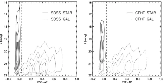
Figure 8.Comparison of the star/galaxy separator used in the PS1 MD catalogs (thick dashed lines) to matches in the SDSS (left) and CFHT (right) archival catalogs in the PS_GROTH field as a function ofi-band magnitude.
Deep stacks of the multi-epoch observations were generated to provide deep imaging with a 5σ point-source limiting magnitude of∼24.9, 24.7, 24.7, 24.3, and 23.2 mag in thegP1,
rP1, iP1, zP1, and yP1 bands, respectively, and typical seeing
(PSF FWHM) of ∼1.4,1.3,1.0,1.0, and 1.0 in the five bands, respectively. The magnitudes are in the “natural” Pan-STARRS1 system,m= −2.5log(flux)+m, with a relative zero-point adjustment m made in each band for each individual epoch (Schlafly et al.2012) before stacking to conform to the absolute flux calibration in the AB magnitude system (Tonry et al. 2012). We convert the PS1 magnitudes to the SDSS system using the bandpass transformations measured for stellar spectral energy distributions in Tonry et al. (2012), and correct for Galactic extinction using the Schlegel et al. (1998) dust map values forE(B−V) listed in Table2. We obtain morphology information from the PS1 IPP output parameters in the iP1
filter for the PSF magnitude (PSF_INST_MAG), the aperture magnitude (PSF_AP_MAG), and the PSF-weighted fraction of unmasked pixelsPSF_QF, to define a point source or extended source as:
IF PSF INST MAG–PSF AP MAG< 0.04 magAND PSF QF
> 0.85THENclass=pt
IF PSF INST MAG–PSF AP MAG>0.04 magAND PSF QF
>0.85THENclass=ext We calibrated these parameter cuts by comparing sources detected in both the PS1 MDS and archival optical catalogs. Figure 8 shows the PS1 star/galaxy separation criteria for 110,804 sources detected in both PS1 and SDSS catalogs in the PS_GROTH field, and for 169,461 sources detected in both PS1 and CFHT catalog in the PS_GROTH field, withi <22 mag, the faintest magnitude for 96% of the optical hosts of theGALEX TDS sources, and the magnitude limit where all three catalogs are complete. Even though the CFHT catalogs are deeper than SDSS, they do not attempt to separate stars and galaxies for
i21 mag, and classify all sources fainter than this magnitude as point sources. However, it is clear from both comparison plots, that the PS1 criterion ofPSF_INST_MAG−PSF_AP_MAG
<0.04 mag does an even better job of separating the locus of stars from galaxies than both catalogs down toi∼22 mag.
4.3. Archival Redshift and X-Ray Catalogs
We also take advantage of the many archival X-ray and spectroscopic catalogs available from the overlap of theGALEX TDS survey with legacy survey fields. In the PS_CDFS field we us X-ray catalogs from the 0.3 deg2ChandraExtended CDFS
survey (Giacconi et al.2002; Lehmer et al.2005; Virani et al.
2006), and redshift catalogs from the VIMOS VLT Deep Survey (VVDS; Le F`evre et al. 2004), and a compilation of redshift catalogs from GOODS and SWIRE.11 In the PS_XMMLSS field we use X-ray catalogs from the 5.5 deg2XMM-LSS survey
(Chiappetti et al.2005; Pierre et al.2007), and redshift catalogs from VVDS (Le F`evre et al.2005). In the PS_COSMOS field, we use X-ray catalogs from the 1.9 deg2 XMM-Newton Wide-Field Survey (Hasinger et al.2007) and the 0.9 deg2 Chandra
COSMOS survey (Elvis et al. 2009), and redshifts from the Magellan COSMOS AGN survey (Trump et al. 2007,2009), the VLT zCOSMOS bright catalog (Lilly et al.2007,2009), and the Chandra COSMOS Survey catalog (Civano et al. 2012). In the PS_GROTH field we use X-ray catalogs from the 0.67 deg2 ChandraExtended Groth Strip (Nandra et al.2005; Laird et al.2009) and redshift catalogs from the DEEP2 Galaxy Redshift Survey (Newman et al.2012). For PS_ELAISN1 we use the X-ray catalog from the 0.08 deg2 ChandraELAIS-N1
deep X-ray survey (Manners et al.2003). Figure1shows the overlap of the GALEX TDS fields with the archival X-ray surveys. Finally, we also match the sources with the ROSAT All-Sky Bright Source and All-Sky Survey Faint Source catalogs (Voges et al.1999,2000).
5. CLASSIFICATION
We classify theGALEX TDS sources using a combination of optical host photometry and morphology, UV variability statistics, and matches with archival X-ray and redshift catalogs. Table3summarizes the sequence of steps we use to classify the sources, which we describe in detail below.
5.1. Cross-match with Optical Catalogs
We first cross-matched our 1078GALEXTDS sources with the archivalu, g, r, i, zcatalogs described in Section4.1with a
11 http://www.eso.org/sci/activities/garching/projects/goods/
Figure 9.Left: histogram ofrmagnitudes of optical matches. Right: histogram of NUV−rcolors of optical matches for those sources detected in the NUV during their low-state (solid lines), and those sources with upper limits during their low-state (dashed lines).
Table 3
GALEXTDS Classifications
Step Nunclass Archive PS1 Classification Pt Gal
Pt Ext Pt Ext Orphan QSO RRL Mdw Star AGN
Optical match 1078 487 391 76 103 21
QSO color cut 1078 326 326
RRL color cut 753 37 37
Mdw color cut 716 44 9 53
Stellar locus color cut 663 17 17
Syr/Sd3 646 19 15 34
Stochastic UV var 616 200 68 268
X-ray/spec match 346 8 37 2 5 37
302 21 358 37 53 22 305 93 189
matching radius of 3. This radius is recommended for matches betweenGALEXand ground-based optical catalogs (Budav´ari & Szalay2008), and corresponds to a spurious match rate of only 1%–2% at the high Galactic latitudes of theGALEXTDS fields (Bianchi et al.2011). However, we found that there was a population of “orphans” (no optical match within 3) that were detected in their NUV low-state, and had a match between 3–4 with an optically identified quasar. Given the strong likelihood that these are real matches, we increased our matching radius to 4. We use the star/galaxy classifications from the catalogs to label sources as point sources (pt) or extended sources (ext). This results in 878/1078 optical matches (81%), with the majority of sources without matches in PS_CDFS, which is only partially covered by the archival catalogs.
We then match the sources that do not have archival optical matches to the PS1 MDS catalog described in Section4.2, this increases the number of sources with optical photometry and morphology (albeit without theu band) to 1057/1078 (98%). Figure 9 shows a histogram of the r-band magnitude of the optical hosts, and the NUV−r colors of the GALEX TDS sources in their low-state. The optical hosts have a distribution that peaks atr∼21 mag, over 3 mag brighter than the detection limit of PS1 MDS, and NUV−r∼1 mag. Sources not detected in their NUV low-state are shown as upper limits in the NUV−r
color histogram, and peak at NUV−r >2 mag. 5.2. Orphans
We visually inspected the PS1 stack images at the locations of the 21 sources with no optical matches, and confirm that
they are true orphan events. Furthermore, all of the orphans are undetected in their low-state in the NUV, with upper limits of NUV >(22.3–23.1) mag. Thus the orphan hosts are likely distant stars or faint galaxies (i.e., dwarf galaxies or high-redshift galaxies) that are undetected during their low-state in the optical andNUV.
5.3. Color and Morphology Cuts
We first use the color and morphology of the optical hosts to classify theGALEX TDS 5σ UV variable sources. We define quasars as sources with optical point-source hosts with
u−g <0.7
−0.1< g−r <1.0 (3)
in order to avoid the stellar locus and white dwarfs (Richards et al.2002). Note that this color selection can be contaminated by cataclysmic variable stars (CVs), which overlap in color–color space with the quasar sample. Indeed, two of the sources clas-sified by color as quasars are in fact spectroscopically con-firmed CVs (VVDS22H_MOS05-05 and ELAISN1_MOS15-02). VVDS22H_MOS05-05 is ROTSE3 J221519.8-003257.2, a confirmed cataclysmic variable star with a dwarf-nova type spectrum. We observed ELAISN1_MOS15-02 with the APO 3.5 m telescope Dual Imaging Spectrograph (DIS) on 2011 May 3 and detected broad Balmer emission lines from a Galac-tic source, characterisGalac-tic of a CV/dwarf nova spectrum. While these sources stood out easily because of their extreme magni-tude of variability of|Δm|>4 mag, shown in Figure10, there
Figure 10.Maximum NUV variability amplitude as a function of low-state NUV magnitude for sources classified as RR Lyrae (red), M dwarfs (yellow), quasars (blue) AGN (green), and CVs (cyan). Dashed line shows the median 5σ error selection function used to select the variable sources.
(A color version of this figure is available in the online journal.)
may be lower amplitude CV events still hiding in our quasar sample. However, given the low surface density of CVs rela-tive to quasars in the sky (Szkody et al.2011), the expected contamination rate is consistent with the two CVs identified.
We define RR Lyrae stars as sources with optical point source hosts with
0.75< u−g <1.45
−0.25< g−r <0.4
−0.2< r−i <0.2
−0.3< i−z <0.3 (4)
(Sesar et al.2010). Note that the color cuts for quasars and RR Lyrae require theu-band, which is not available for sources with PS1-only matches. However, we define M dwarf stars as point sources with r−i >0.42 (5) i−z >0.24 g <22.2 r <22.2 i <21.3 (6)
(West et al. 2011), which does not require u-band data. We classify stars on the main stellar locus as those with
1.0< u−g <2.25 0.4< g−r <1.0
−0.2< r−i <2.0
−0.3< i−z <1.0 (7)
modified from Yanny et al. (2009). This color and morphology selection results in 37 RR Lyrae, 53 M-dwarf flare stars, 17 stars, and 325 quasars. Figure11shows the optical color–color diagram of the sources with optical point-source hosts and u-band data, and their classifications as quasars, RR Lyrae, M dwarfs, and stars.
Figure 11.Colors of archival optical matches to UV variable sources with point-like optical hosts (black points). Dashed blue line shows the region in color–color space used to define quasars from optical colors and morphology alone. Sources with classification are color coded as quasars in blue, RR Lyrae in red, and M dwarf stars in yellow, and main stellar locus stars in cyan. Sources with archival X-ray matches are circled in purple.
(A color version of this figure is available in the online journal.)
Figure 12.Histogram of the NUV structure function of sources classified as RR Lyrae (red) and quasars (blue) on a timescale of days and years. The red and blue arrows indicate the mean ofSyrmeasured in the SDSSr-band for RR Lyrae and quasars, respectively, from Schmidt et al. (2010).
(A color version of this figure is available in the online journal.)
5.4. UV Variability Cuts
Figure12shows the structure function on timescales of days and years described in Section3for the sources classified as RR Lyrae and quasars in Section5.3. In Figure13we show the ratio of the NUV structure function on timescales of years to days (Syr/Sd). While quasars demonstrate a wide range ofSyr/Sd, all
RR Lyrae haveSyr/Sd<3. We use this UV variability property
to relax our color constraints, and increase our photometric sample of quasars to all sources with optical point-source hosts
Figure 13.Histogram of the ratio of the NUV structure function on timescales of years and days for sources classified as RR Lyrae (red) and quasars (blue). The dotted line shows the selection criteria ofSy/Sd3 used to classify sources with optical point source hosts as quasars.
(A color version of this figure is available in the online journal.)
Figure 14.Colors of archival optical matches to UV variables with extended optical hosts. Sources classified as AGN (by either stochastic UV variability, archival spectra, and/or an X-ray match) are color coded in green. Sources with matches with archival X-ray matches are circled in purple. Note that all galaxy sources with an archival X-ray match are defined as AGNs.
(A color version of this figure is available in the online journal.)
with Syr/Sd 3. This is equivalent to a structure function
power-law exponent cut of γ > 0.2, where S(Δt) ∝ Δtγ
(Hook et al. 1994; Vanden Berk et al. 2004; Schmidt et al.
2010). This structure-function ratio selection results in the classification of another 30 quasars. Two additional sources with optical point-source hosts have archival quasar spectra, resulting in a final quasar sample of 358. We define AGNs as sources with optically extended hosts that show stochastic UV variability (see Section3.3), have an X-ray catalog match, and/or an archival spectroscopic classification. Figure14shows the optical color–color diagram of the sources with optically extended hosts, and those classified as AGN. This results in a sample of 305 AGNs. We also add archival spectroscopic classifications for six stars. This yields a total of 776/1078 (72%) sources classified as an active galaxy (quasar or AGN) or variable star.
cation. The dashed blue line shows the median 5σvariability selection function as a function of mean magnitude. The nature of the optical host is indicated (point source, galaxy, or orphan), and flaring sources (including transients) are marked in yellow.
(A color version of this figure is available in the online journal.)
5.5. X-Ray Sources
The archival X-ray catalogs overlap with∼8.45 deg2 of the GALEX TDS survey area. Within this area, 81/89 quasars, 92/105 AGNs, and 8/9 M-dwarf stars are detected in the X-rays. In addition, there are nine optical point sources with X-ray matches that are likely quasars and M dwarfs just outside the quasar and M-dwarf color–color selection regions. UV variability selection appears to be selecting a similar population of active galaxies and M dwarfs as X-ray detection, since∼90% of the UV variability-selected active galaxy and M dwarf sample is also detected in the X-rays. However, only 2% of all the X-ray sources (the majority of which are active galaxies) are detected as UV variable at the selection threshold of theGALEXTDS catalog.
5.6. GUVV Catalog
We also cross-match ourGALEXTDS sample with the first and secondGALEXUltraviolet Variability Catalogs (GUVV-1 and GUVV-2) from Welsh et al. (2005) and Wheatley et al. (2008). These catalogs include 894 UV variable sources (Δm >
0.6 mag in the NUV) selected from an analysis of archival GALEXAIS, MIS, DIS, and Guest Investigator (GI) fields with repeated observations. With a cross-matching radius of 4, we find a match with 36 GUVV sources. For the 15 matches that have GUVV classifications, are all classified by GUVV as active galaxies (AGN or quasar), which are in agreement with our GALEXTDS classifications. Of the 21 matches without GUVV classifications, we find 5 sources classified byGALEXTDS as RR Lyrae, 9 classified as active galaxies (AGN or quasar), 6 with optical point-source hosts, and 1 with a galaxy host.
5.7. Unclassified Sources
The remaining 302 unclassified sources include 91 with optical point-source hosts, which are likely stars, quasars with non-standard colors (high-redshift or reddened), or unresolved galaxies, 190 with galaxy hosts, and 21 orphans. The 190 galaxy hosts may either be faint AGNs with poorly constrained UV light curves, or hosts of UV-bright extragalactic transients. In Figure15we show the maximum|Δm|in the NUV as a function of low-state NUV magnitude of the remaining unclassified sources. The unclassified UV source with the most extreme amplitude, ELAISN1_MOS15-09 with|Δm| > 4.2 mag, was
− · · ·
COSMOS_MOS22-11 149.4973 3.1171 22.56 3.35 0.75 · · · 0.58 F pt 14.25 Mdw Mdw
GROTH_MOS05-00 214.9435 52.9953 22.07 3.29 0.71 1.18 0.65 F pt 14.15 Mdw X Mdw
XMMLSS_MOS06-22 36.6468 −5.0886 >22.95 >3.28 0.95 <0 4.04 pt 15.58 Mdw X Mdw
(This table is available in its entirety in a machine-readable form in the online journal. A portion is shown here for guidance regarding its form and content.)
spectroscopically confirmed to be from the nucleus of an inactive galaxy at z = 0.1696, and its UV/optical flare detected by GALEX TDS and PS1 MDS (PS1-10jh) was attributed to the tidal disruption of a star around an SMBH (Gezari et al. 2012). Also in this sample is a UV transient spectroscopically confirmed to be a Type IIP SN 2010aq at
z = 0.086 (COSMOS_MOS26-29), whose UV/optical light curve fromGALEX TDS and PS1 MDS was fitted with early emission following SN shock breakout in a red supergiant star (Gezari et al.2010). Both of these spectroscopically classified extragalactic transients are labeled in Figure15.
Our 5σselection criteria translates to a limiting sensitivity to transients in a host galaxy with a magnitudemhostof a magnitude
of mtrans = −2.5 log 10mhost−−52σ.5(mhost )−10 mhost −2.5, (8)
which ranges frommtrans ∼ 20.0 mag formhost = 18 mag to
mtrans ∼ 22.7 mag formhost = 23 mag. Thus, our variability
selection threshold is less sensitive to transients in host galaxies with bright NUV fluxes. On the red sequence of galaxies, where
MNUV ≈ −14.5 (Wyder et al. 2007), this selection effect is
not as much of an issue, since already forz > 0.05 one gets mhost > 22 mag. However, star-forming galaxies on the blue
sequence are 2.5 mag brighter in the NUV, and thus the host galaxy brightness can be a factor in reducing the sensitivity to faint transients. For example, ourGALEX TDS 5σ sample does not include SN 2009kf, a luminous Type IIP SN in a star-forming galaxy atz = 0.182 which we reported our GALEX TDS detection of in Botticella et al. (2010). This source varied at only the 4.25σ level in the NUV during its peak. However, because this transient was selected from a spatial and temporal coincidence with a PS1 transient alert, we could lower our threshold for variability selection in the UV. The systematic selection of SN and TDE candidates from the joint GALEX TDS and PS1 MDS transient detections will be presented in future papers.
6. DISCUSSION 6.1. Classification Demographics
Figure16shows a pie diagram of the source classifications. Out of the total of 1078GALEXTDS sources, 62% are classified as actively accreting SMBHs (quasars or AGN), and 10% as variable and flaring stars (including RR Lyrae, M dwarfs, and CVs). Note that the relative fraction of the different classes of sources is sensitive to both their intrinsic magnitude distribution, and the magnitude-dependent variability selection function of
Figure 16.Pie chart ofGALEXTDS classifications: sources classified as stars (Star), M dwarfs (Mdw), RR Lyrae (RRL), quasars (QSO), and active galactic nuclei (AGN), and sources with no classification with galaxy hosts (Galaxy), no host (Orphan), and point-source hosts (Point).
(A color version of this figure is available in the online journal.)
the sample. Table 4 gives the GALEX TDS catalog, sorted by decreasing NUV amplitude, with the GALEX ID, R.A., decl., low-state NUV magnitude, maximum amplitude of NUV variability (|Δmmax|), intrinsic variability (σint), the structure
function on day (Sd) and year (Sy) timescales; the characteristics
of the NUV light curve: flaring (F) or stochastically variable (V); the morphology of the matching optical host: point-source (pt) or extended (ext); the color classification of the matching optical host: RR Lyrae (RRL), M dwarf star (Mdw), star (Star), or quasar (QSO); the archival redshift, an X mark if there is a match with an archival X-ray source; and finally theGALEX TDS classification: RR Lyrae (RRL), M dwarf star (Mdw), star (star), quasar (QSO), AGN, UV flaring source or UV transient source with galaxy host (Galaxy Flare or Galaxy Trans), UV flaring source or transient source with point-source optical host (Point Flare or Point Trans) or UV flaring source or transient source with orphan optical host (Orphan Flare or Orphan Trans), stochastically variable source with a point-source optical host (Point Var), stochastically variable orphan (Orphan Var), or none of the above (?).
In Figure17we show the cumulative surface density distribu-tion of classified UV variable sources as a funcdistribu-tion of peak mag-nitude (high(NUV)) and maximum amplitude (max(|ΔNUV|)). For the variable UV sources, these correspond to total surface densities of 8.0±3.1, 7.7±5.8, and 1.8±1.0 deg−2for quasars,
Figure 17.Cumulative distribution of surface density of UV variable sources withGALEXTDS classifications: M dwarfs (Mdw), RR Lyrae (RRL), quasars (QSO), active galactic nuclei (AGN), and extragalactic transients (GAL-Flare) as a function of peak magnitude (high(NUV), left) and maximum amplitude (max(|ΔNUV|)). (A color version of this figure is available in the online journal.)
Figure 18.Intrinsic NUV variability as a function of low-state NUV magnitude for sources classified as RR Lyrae (red), M dwarfs (yellow), quasars (blue) and AGN (green). Arrows shows the medianσintmeasured in the optical for quasars (blue arrow), RR Lyrae (red arrow), and M dwarfs (orange arrow) from Sesar et al. (2007).
(A color version of this figure is available in the online journal.)
AGNs, and RR Lyrae, respectively. For the transient sources, we can calculate a total surface density rate, #/(area×teff), where
teff is the effective survey time at the cadence that matches the
characteristic timescale of the transient. For extragalactic tran-sients such as young SNe and TDEs, which vary on a timescale of days, we use the time intervals for which the fields were ob-served with a cadence of 2.0±0.5 days. If we include all flaring or transientGALEXTDS sources with a galaxy host, this yields a surface density rate of 52±38 deg−2yr−1 for extragalactic
transients. For M dwarfs which vary on timescales shorter than an individual observation, we use the total exposure time for each epoch. If we assume a survey with a cadence of two days andtexp=1.5 ks, this translates to a surface density rate for M
dwarfs of 15±10 deg−2yr−1.
6.2. UV Variability Properties of Classified Sources Various optical studies of rest-frame UV variability in high redshift quasars have demonstrated that the variability of AGN increases with decreasing rest wavelength (di Clemente et al.
1996; Vanden Berk et al.2004; Wilhite et al.2005). In Figure18, we show histograms ofσint for the UV variable sources with
classifications. Quasars show a distribution ofσintwith a mean
that is ∼2 times larger than measured at optical wavelengths from the SDSS Stripe 82 sample from Sesar et al. (2007). This effect is even more pronounced in the magnitude of the structure function on years timescales (Sy), which has a mean that is five
times larger than the mean measured in ther-band (λeff =6231)
from Schmidt et al. (2010). This trend is consistent with the wavelength-dependent rise in variability amplitude observed in the structure function for quasars in the rest-frame UV (Vanden Berk et al.2004) and observed UV (Welsh et al.2011).
The fact that AGN become bluer during high states of flux (Giveon et al. 1999; Geha et al. 2003; Gezari et al.
2008a) has been attributed to increases in the characteristic temperature of the accretion disk in response to increases in the mass accretion rate (Pereyra et al.2006; Li & Cao2008). However, Schmidt et al. (2012) argue that the color variability observed inindividualquasars in their SDSS Stripe 82 sample is stronger than expected from just varying the accretion rate (M˙) in accretion disk models. In a future study, we will use simultaneous UV and optical light curves from GALEXTDS and PS1 MDS for our 358 individual quasars to test this result with a larger dynamic range in wavelength.
For the subsample of 95 quasars with archival redshifts (zmean=1.26,σz=0.39), in Figure19we plotσintversus the
low-state NUV absolute magnitude, and find a steep negative correlation fitted by log(σint) = (1.6±0.1) + (β/2.5)MNUV,
whereβ =0.24±0.04, in excellent agreement with the trend for increased variability in lower luminosity quasars seen from optical observations with β = 0.246±0.005 (Vanden Berk et al. 2004), and shallower than expected for a Poissonian process which has β = 0.5 (Cid Fernandes et al. 2000). We also show the subset of 68 AGN with archival redshifts (zmean=0.64,σz=0.55), which clearly do not show a relation
between σint and low-state NUV absolute magnitude. This is
most likely a result of dilution of the variability amplitude from the contribution of the host galaxy in the NUV.
The largest values of|Δm|(plotted in Figure10) are found in RR Lyrae and M dwarfs, with a tail of large amplitude variations reaching up to |Δm| = 2.9 mag in RR Lyrae and up to |Δm| = 4.6 mag in M dwarfs. In the optical, the RR Lyrae structure function is very weakly dependent on timescale, with an amplitude of 0.1–0.2 mag (Schmidt et al. 2010). The NUV structure function also shows a weak dependence of amplitude on timescale when comparing the structure function on days to years timescales, however, with an amplitude that is
Figure 19.Intrinsic NUV variability as a function of low-state NUV absolute magnitude,MNUV=low(NUV)−DM where DM is the distance modulus, for the subsample of quasars (blue dots) and AGNs (green circles) with catalog redshifts. Dashed blue line shows the fit to the quasars to log(σint)∝(β/2.5)M. The spectroscopically classified extragalactic transients (TDE PS1-10jh and SN 2010aq) are labeled.
(A color version of this figure is available in the online journal.)
∼3 times larger in the NUV than in the optical. This wavelength dependence on variability amplitude can be explained if the variability is driven by variations in surface temperature from pulsations of the stellar envelope, where higher states of flux are associated with higher temperatures (Sesar et al.2007).
7. CONCLUSIONS
We provide a catalog of over a thousand UV variable sources and their classifications based on optical host properties, UV variability behavior, and cross-matches with archival X-ray and redshift catalogs. This yields a sample of 53 M dwarfs, 37 RR Lyraes, 358 quasars, and 305 AGNs. We find median intrinsic UV variability amplitudes in RR Lyrae and quasars that are factors of>3 larger than at optical wavelengths, consistent with the expectation for higher temperatures during higher states of flux. The regular cadence and wide area ofGALEX TDS enables us to systematically discover persistent and transient (i.e., tidal disruption of a star) accreting SMBHs over wide fields of view, study the contemporaneous UV and optical variability of variable stars, and catch young core-collapse SNe within the first days after explosion. The overlap of theGALEXTDS with PS1 MDS and multiwavelength legacy survey fields will continue to be helpful for classifying transient sources in these heavily observed fields. We also measure the surface densities of variable sources and the surface density rates for transients as a function of class in the UV for the first time.
WithGALEXTDS we are only scratching the surface of UV variability. Our 5σsample of 1078 sources is less than 0.3% of the 419,152 UV sources in the field (with an average density of 1.1×10⁴UV sources per square degree down tom
lim=23 mag).
Looking to the future, the discovery rate for UV variable sources and UV transients could increase byseveralorders of magnitude with the launch of a space-based UV mission with a wide field of view (several deg2), a survey strategy of daily cadence
observations over∼100 deg2, and detectors with an order of
magnitude improved photometric precision relative toGALEX. In the optical sky, 90% of quasars vary withσint >0.03 mag
on the timescales of years (Sesar et al.2007). Given the factor of∼2 largerσint observed for quasars in the NUV, one could achieve a nearly complete sample of low-redshift quasars with
April. We gratefully acknowledge NASA’s support for construc-tion, operaconstruc-tion, and science analysis for the GALEXmission, developed in cooperation with the Centre National d’Etudes Spatiales of France and the Korean Ministry of Science and Technology. The Pan-STARRS1 survey has been made possible through contributions of the Institute for Astronomy, the Univer-sity of Hawaii, the Pan-STARRS Project Office, the Max Planck Society and its participating institutes, the Max Planck Institute for Astronomy, Heidelberg and the Max Planck Institute for Extraterrestrial Physics, Garching, The Johns Hopkins Univer-sity, Durham UniverUniver-sity, the University of Edinburgh, Queen’s University Belfast, the Harvard-Smithsonian Center for Astro-physics, and the Las Cumbres Observatory Global Telescope Network, Incorporated, the National Central University of Taiwan, and the National Aeronautics and Space Administration under grant No. NNX08AR22G issued through the Planetary Science Division of the NASA Science Mission Directorate.
REFERENCES
Aihara, H., Allende Prieto, C., An, D., et al. 2011,ApJS,193, 29
Bianchi, L., Efremova, B., Herald, J., et al. 2011,MNRAS,411, 2770
Botticella, M. T., Trundle, C., Pastorello, A., et al. 2010,ApJL,717, L52
Brown, P. J., Holland, S. T., Immler, S., et al. 2009,AJ,137, 4517
Budav´ari, T., & Szalay, A. S. 2008,ApJ,679, 301
Burgett, W. S. 2012,Proc. SPIE,8449, 84490T
Chevalier, R. A., & Irwin, C. M. 2011,ApJL,729, L6
Chiappetti, L., Tajer, M., Trinchieri, G., et al. 2005,A&A,439, 413
Cid Fernandes, R., Sodr´e, L., Jr., & Vieira da Silva, L., Jr. 2000,ApJ,544, 123
Civano, F., Elvis, M., Brusa, M., et al. 2012,ApJS,201, 30
di Clemente, A., Giallongo, E., Natali, G., Trevese, D., & Vagnetti, F. 1996,ApJ,
463, 466
Elvis, M., Civano, F., Vignali, C., et al. 2009,ApJS,184, 158
Geha, M., Alcock, C., Allsman, R. A., et al. 2003,AJ,125, 1
Gezari, S., Basa, S., Martin, D. C., et al. 2008a,ApJ,676, 944
Gezari, S., Chornock, R., Rest, A., et al. 2012,Natur,485, 217
Gezari, S., Dessart, L., Basa, S., et al. 2008b,ApJL,683, L131
Gezari, S., Heckman, T., Cenko, S. B., et al. 2009,ApJ,698, 1367
Gezari, S., Martin, D. C., Milliard, B., et al. 2006,ApJL,653, L25
Gezari, S., Rest, A., Huber, M. E., et al. 2010,ApJL,720, L77
Giacconi, R., Zirm, A., Wang, J., et al. 2002,ApJS,139, 369
Giveon, U., Maoz, D., Kaspi, S., Netzer, H., & Smith, P. S. 1999,MNRAS,
306, 637
Hasinger, G., Cappelluti, N., Brunner, H., et al. 2007,ApJS,172, 29
Hook, I. M., McMahon, R. G., Boyle, B. J., & Irwin, M. J. 1994, MNRAS,
268, 305
Huber, M., Rest, A., Narayan, G., et al. 2011, BAAS, 43, 328.12
Kaiser, N., Burgett, W., Chambers, K., et al. 2010,Proc. SPIE, 7733, 77330E Kowalski, A. F., Hawley, S. L., Hilton, E. J., et al. 2009,AJ,138, 633
Laird, E. S., Nandra, K., Georgakakis, A., et al. 2009,ApJS,180, 102
Le F`evre, O., Vettolani, G., Garilli, B., et al. 2005,A&A,439, 845
Le F`evre, O., Vettolani, G., Paltani, S., et al. 2004,A&A,428, 1043
Lehmer, B. D., Brandt, W. N., Alexander, D. M., et al. 2005,ApJS,161, 21
Li, S.-L., & Cao, X. 2008,MNRAS,387, L41
Lilly, S. J., Le Brun, V., Maier, C., et al. 2009,ApJS,184, 218
Lilly, S. J., Le F`evre, O., Renzini, A., et al. 2007,ApJS,172, 70
Schlafly, E. F., Finkbeiner, D. P., Juri´c, M., et al. 2012,ApJ,756, 158
Schlegel, D. J., Finkbeiner, D. P., & Davis, M. 1998,ApJ,500, 525
Schmidt, K. B., Marshall, P. J., Rix, H.-W., et al. 2010,ApJ,714, 1194
Schmidt, K. B., Rix, H.-W., Shields, J. C., et al. 2012,ApJ,744, 147
Sesar, B., Ivezi´c, ˇZ., Grammer, S. H., et al. 2010,ApJ,708, 717
Wheatley, J., Welsh, B. Y., & Browne, S. E. 2012,PASP,124, 552
Wheatley, J. M., Welsh, B. Y., & Browne, S. E. 2008,AJ,136, 259
Wilhite, B. C., Vanden Berk, D. E., Kron, R. G., et al. 2005,ApJ,633, 638
Wyder, T. K., Martin, D. C., Schiminovich, D., et al. 2007,ApJS,173, 293