Diversity Comparison of Pareto Front
Approximations in Many-Objective Optimization
Miqing Li, Shengxiang Yang
Member, IEEE,
and Xiaohui Liu
Abstract—Diversity assessment of Pareto front approximations is an important issue in the stochastic multiobjective optimization community. Most of the diversity indicators in the literature were designed to work for any number of objectives of Pareto front approximations in principle, but in practice many of these indicators are infeasible or not workable when the number of objectives is large. In this paper, we propose a Diversity Comparison Indicator (DCI) to assess the diversity of Pareto front approximations in many-objective optimization. DCI evaluates relative quality of different Pareto front approximations rather than provides an absolute measure of distribution for a single approximation. In DCI, all the concerned approximations are put into a grid environment so that there are some hyperboxes containing one or more solutions. The proposed indicator only considers the contribution of different approximations to non-empty hyperboxes. Therefore, the computational cost does not increase exponentially with the number of objectives. In fact, the implementation of DCI is of quadratic time complexity, which is fully independent of the number of divisions used in grid. Systematic experiments are conducted using three groups of artificial Pareto front approximations and seven groups of real Pareto front approximations with different numbers of objectives to verify the effectiveness of DCI. Moreover, a comparison with two diversity indicators used widely in many-objective optimiza-tion is made analytically and empirically. Finally, a parametric investigation reveals interesting insights of the division number in grid and also offers some suggested settings to the users with different preferences.
Index Terms—Multiobjective optimization, many-objective op-timization, performance assessment, diversity comparison indi-cator.
I. INTRODUCTION
M
ANY real-world problems involve simultaneous opti-mization of several competing criteria or objectives: often, there is no single optimal solution, but rather a set of Pareto optimal solutions (also called Pareto front in the objective space). In general, generating the Pareto front is often infeasible, since the complexity of the underlying appli-cation prevents exact methods from being applicable. Heuristic search methods are an alternative: they try to find a good Manuscript received September 5, 2013; revised December 29, 2013; ac-cepted February, 26, 2014. This work was supported in part by the Engineering and Physical Sciences Research Council (EPSRC) of U.K. under Grant EP/K001310/1, National Natural Science Foundation of China (Major Inter-national Joint Research Project) under Grant 71110107026, EU FP7-Health under Grant 242193, EPSRC Industrial Case under Grant 11220252, and the Education Department and “Qinglan Engineering” of Jiangsu Province, China. M. Li and X. Liu are with the Department of Information Systems and Computing, Brunel University, Uxbridge, Middlesex UB8 3PH, U. K. (email: {miqing.li, xiaohui.liu}@brunel.ac.uk).S. Yang is with the Centre for Computational Intelligence (CCI), School of Computer Science and Informatics, De Montfort University, Leicester LE1 9BH, U. K. (e-mail: [email protected]).
approximation that is not too far away from the Pareto front, although they usually do not guarantee to obtain the optimal tradeoffs. Over the past decades, various stochastic heuristic search techniques, such as genetic algorithms, particle swarm optimization algorithms, ant colony optimization algorithms, simulated annealing, and tabu search, have been proposed to solve multiobjective optimization problems (MOPs), and their usefulness has been demonstrated in many application domains [1]–[5].
With the rapid development of useful and effective tech-niques in multiobjective optimization, the issue of perfor-mance assessment has become increasingly important and has developed into an independent research topic. Numerous quality indicators [6]–[10] have been emerging in the literature to evaluate the performance of Pareto front approximations obtained by multiobjective optimizers. They mainly concen-trate on three aspects that the optimizers try their best to optimize: 1) the convergence of the obtained approximation, 2) the uniformity of the approximation, and 3) the spread (i.e., extensity) of the approximation. The latter two are closely related aspects, and in general, they are called the diversity of the approximation.
Many-objective optimization problems, which appear widely in industrial and engineering design [11]–[13], usually refer to those problems with more than three objectives. In recent years, many-objective optimization has been gaining increasing attention in the stochastic multiobjective optimiza-tion community: a great variety of many-objective optimizers have been developed [14]–[19], and their performance has been tested on many problems with different characteristics [20]–[25].
However, how to compare the Pareto front approximations obtained by different many-objective optimizers seems having not gotten enough attention and concern [26], which largely hinders the deep investigation of the performance of optimizers [27], [28]. Most of the quality indicators that are scalable analytically to any number of objectives are often not available actually to the problems with a large number of objectives. In general, the difficulties of comparing many-objective Pareto front approximations may be mainly attributed to three rea-sons, which are summarized as follows.
• Visual comparison of approximations. When the number of objectives of Pareto front approximations is more than three, visual and intuitive quality assessment can be misleading or even impossible, despite the fact that it is a prevailing comparison tool in the literature.
• Substitution of the Pareto front. Many quality indicators need to compare an approximation with a reference set,
which is regarded as a substitution of the Pareto front. Due to the “curse of dimensionality”, the number of points required to accurately represent the Pareto front of a given problem increases exponentially with the number of objectives. This places the setting of the number of points in a reference set in a dilemma: a large number will pose a challenge to the storage and access of data, whereas a small one will decrease the accuracy of the evaluation results.
• Complexity of storage and time. The storage or time requirement of some quality indicators, such as hy-pervolume [29], diversity measure [30], and hyperarea difference [31], increases exponentially with the number of objectives. This may limit their applicability in per-formance comparison of high-dimensional Pareto front approximations.
Whereas the above difficulties have created obstacles to the design of quality indicators in many-objective optimiza-tion, the influence for indicators on different aspects (i.e., convergence and diversity) may be of great difference. Some convergence indicators can avoid these difficulties by utilizing the characteristics of the Pareto front of the considered test problems [32], [33] or by testing the dominance relation between individuals of different approximations [9], [14], etc. However, for diversity indicators, a proper reflection of the distribution of approximations seems to be more difficult in many-objective optimization [7]. Separate assessment of uniformity and spread may give a misleading result about the whole distribution of an approximation (a detailed ex-planation will be given in the next section). In general, a diversity indicator without the introduction of comparison between an approximation and the problem’s Pareto front fails to accurately reflect the distribution of the approximation, since the true shape and distribution of the optimal front are often unknown beforehand and hard to estimate in a high dimensional space.
In this paper, we propose a diversity1 comparison
indica-tor (DCI) to compare Pareto front approximations in many-objective optimization. DCI assesses the relative quality of different Pareto front approximations rather than provides an absolute measure of distribution for a single approximation, so that a reference set that is difficult to accurately represent the Pareto front of a many-objective optimization problem is not needed. Moreover, unlike binary quality indicators [34], [35], which compare the performance of two approximations, DCI is available for any number of approximations, which seems very attractive because it can identify all the considered approximations in a single run.
The rest of this paper is organized as follows. In Section II, the related work is reviewed and discussed. Section III is devoted to the description of the proposed performance indicator. Empirical comparative studies and discussions are presented in Section IV. Finally, Section V provides some concluding remarks along with pertinent observations.
1This paper focuses on the diversity in the objective space, rather than in the variable space, although the latter is also very important in the area.
II. RELATEDWORK
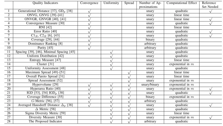
During the past decade, various quality indicators have been emerging in the stochastic multiobjective optimization domain [7], [9], [36]. Some of them focus on the performance of Pareto front approximations in terms of a single aspect, and the others assess several aspects of the quality of approximations. Table I summarizes some quality indicators and their prop-erties, listing the quality aspect(s) involved by the indicators, the number of approximations handled by the indicators, the computational effect needed by the indicators, and the state whether a reference set is required by the indicators or not.
As can be seen from Table I, there are three categories of existing quality indicators regarding the uniformity and spread of Pareto front approximations. The first category separately assesses the uniformity or spread of approximations (items 11– 18), the second one covers all three aspects of performance (i.e., uniformity and spread as well as convergence) (items 19– 24), and the last one focuses on diversity (i.e., both uniformity and spread, but no convergence) (items 25–27).
Considering the first category, although the indicators can separately evaluate the two aspects of diversity, they may fail to reflect the whole distribution of an approximation. Fig. 1 gives a distribution example to explain this case. The solutions of the approximation in the figure are uniformly distributed on the boundary of the Pareto front rather than over the whole Pareto front. In this case, both uniformity indicators (e.g., items 11–15) and spread indicators (e.g., items 16– 18) may give good evaluation results of the approximation. This occurrence can be attributed to the fact that the former only considers distribution uniformity in the neighborhood of solutions (e.g., the Spacing indicator [39] assesses the uniformity of an approximation by calculating the standard deviation of distance from each solution to its closest neighbor in the approximation), and the latter only measures the distri-bution range of boundary solutions rather than the coverage of an approximation to the whole Pareto front [60] (e.g., the Maximum Spread indicator [49] assesses the spread of an approximation by measuring the length of the diagonal of the minimal hyperbox that encloses the approximation). In fact, it may be meaningless that a uniformly-distributed solution set is located only in a small part of the Pareto front, which could be obtained more easily in many-objective optimization due to the exponential growth of the problem space [12], [26].
Note that for accuracy, in the remainder of the paper the meaning of “spread” is modified to refer to the performance of an approximation to cover the whole Pareto front.
The second category of indicators involve all three aspects of performance of approximations, and some of them, such as Hypervolume [29] and Inverted Generational Distance (IGD) [53], are popular to compare multiobjective optimizers in the literature [26], [61], [62]. However, there are some requirements for them to be used, which may obstruct their application in the performance comparison of approximations with a large number of objectives. Although Monte Carlo sampling-based approximate calculation can greatly reduce the computational cost of Hypervolume [63], the proper choice of the reference point in the calculation of the indicator is
TABLE I
QUALITYINDICATORS AND THEIRPROPERTIES Quality Indicators Convergence Uniformity Spread Number of
Ap-proximations
Computational Effect Reference Set Needed
1 Generational Distance [37], GDp[38] √ unary quadratic √
2 ONVG, GNVG [39]–[41] √ unary linear time
3 ONVGR, GNVGR [40], [41] √ unary linear time √
4 Convergence Measure [30] √ unary quadratic √
5 RNI [42] √ unary linear time
6 Error Ratio [40] √ unary quadratic √
7 C1R, C2R [6], [43] √ unary quadratic √
8 Coverage [29], [44] √ binary quadratic
9 Dominance Ranking [8] √ arbitrary quadratic
10 Purity [45] √ arbitrary quadratic
11 Spacing [39], [46], Minimal Spacing [45] √ unary quadratic
12 Uniform Distribution [42] √ unary quadratic
13 Entropy Measure [47] √ unary linear time
14 Cluster [31] √ unary exponential inm
15 Uniformity Assessment [48] √ unary quadratic
16 Maximum Spread [49]–[51] √ unary linear time
17 Overall Pareto Spread [31] √ unary linear time
18 Spread Assessment [52] √ unary exponential inm
19 Hypervolume [29] √ √ √ unary/binary exponential inm
20 Hyperarea Ratio [40] √ √ √ unary exponential inm √
21 IGD [53], [54] IGDp[38] √ √ √ unary quadratic √
22 Coverage Difference [55] √ √ √ binary exponential inm
23 G-Metric [56], [57] √ √ √ arbitrary quadratic
24 Averaged Hausdorff Distance∆p[38] √ √ √ unary quadratic √
25 ∆Metric [58] √ √ unary quadratic
26 Sigma Diversity Metric [59] √ √ unary linear time
27 Diversity Measure [30] √ √ unary exponential inm √
28 The Proposed Indicator √ √ arbitrary quadratic
(a) Pareto front (b) An approximation
Fig. 1. A distribution example that uniformity or spread indicators may fail to reflect the whole distribution of an approximation.
also an important issue [64]. For IGD, a reference set that can accurately represent the Pareto front of a problem is required. Moreover, since these indicators concentrate on an overall consideration of convergence and diversity, they fail to separately reflect the distribution of approximations, which the user may be rather desirous to concern sometimes [65].
In addition, it is interesting to note that the comprehensive performance indicator G-Metric [56] (item 23 in Table I), which measures the convergence and diversity of approxima-tions according to the Pareto dominance relation and “zone of influence” of individuals respectively, could be placed into the third category since their solutions are often mutually non-dominated in a high dimension space. However, since the calculation of “zone of influence” is based on Monte Carlo sampling when more than three objectives are involved, the accuracy of the indicator may be affected as the number of objectives increases.
Represented by ∆ Metric [58], Sigma Diversity Metric
(SDM) [59] and Diversity Measure (DM) [30], the third category of indicators assess the performance of approxi-mations in terms of uniformity and spread. The ∆ Metric is an extension of the uniformity indicator Spacing [39] by considering boundary solutions of the Pareto front for a bi-objective problem, and it is defined as follows:
∆ = df+dl+
∑|P|−1
i=1 di−d¯
df +dl+ (|P| −1) ¯d
(1) where|P|denotes the size of the considered approximationP,
di corresponds to the Euclidian distance between consecutive
solutions inP,d¯stands for the average ofdi, anddf anddl
denote the Euclidian distance between the extreme solution of the Pareto front and the boundary solution in the approxima-tion regarding each of the two objectives, respectively. Due to the introduction of comparison between an approximation and the concerned Pareto front, the∆metric seems to be one that reflects the distribution correctly. Despite the fact that∆
metric can easily be extended in a higher-dimensional space according to the Voronoi diagram approach, how to find the Voronoi diagram of a solution set is not an easy (or even an infeasible) task when more than three objectives are involved. Inspired from the polar and spherical coordinate axis for the 2- and 3-objective space, the SDM indicator assesses the diversity of an approximation by using a set of reference lines dividing the objective space [59]. The outputs of the metric are a percentage of the space and the position information of a given approximation in the space, rather than a scalar value representing the distribution of the approximation. However, due to depending on several parameters, such as the distance
around each reference line, the number of reference lines, and the shape of the Pareto front, the metric may face difficulties to be extended to many-objective optimization.
DM, proposed by Deb at el. [30], has recently been used in some comparison studies of many-objective optimizers [32], [66], [67]. DM measures the diversity of a Pareto front approximation by comparing it with a reference set. In the calculation of DM, the solutions in the approximation are projected on a (m − 1)-dimensional hyperplane which is divided into a number of hyperboxes. The indicator considers each hyperbox and gives it an evaluation value according to the distribution of solutions in it and its neighbors. The more the hyperboxes that, when containing a member of the reference set, also contain a member of the approximation, the higher the indicator value. DM takes the value between zero and one, where one corresponds to the best possible diversity and zero stands for the worst. A more detailed description of DM can be found in [30].
The idea of assessing diversity using a grid-based way is meaningful, but DM has some shortcomings when applied to compare Pareto front approximations with a large number of objectives, which are described as follows:
• A reference set, in which the solutions are uniformly distributed over the Pareto front, is required in order to accurately reflect the distribution of the optimal front; and it is also required that the number of solutions in the reference set is approximate to the number of solutions in the approximation in order to guarantee that the ideal distribution of the approximation can reach the optimal DM value (one). These requirements are often unavailable in many-objective optimization problems.
• DM needs to access each hyperbox in grid to estimate the distribution, which produces great challenges to both the data structure and computational cost. For an opti-mization problem withmobjectives, there will berm−1 hyperboxes to be considered, where r is the number of divisions in each dimension.
• In the distribution estimation for a hyperbox, DM needs to assign each of its neighboring hyperboxes a proper value by a value function to distinguish different distributions of solutions in its neighborhood. Since the number of neighbors of a hyperbox increases exponentially with the number of objectives (there are (3m−1) neighbors for an
m-dimensional hyperbox at most), thevalue function ac-curately reflecting different distributions will be difficult to define when the concerned problem involves a large number of objectives [30].
• DM may fail to give an accurate diversity result of an approximation with a large number of objectives due to the designation of the neighbors of a solution in grid. The setting of neighborhood of a solution in DM is based on the Manhattan distance of grid coordinates of solutions, rather than on the Euclidean distance of them, which may misleadingly eliminate adjacent solutions but regard farther ones as its neighbors (a detailed analysis will be given in Section IV-C).
The diversity indicator proposed in this paper also adopts
a grid-based technique to compare the distribution of Pareto front approximations, but it attempts to solve all the above difficulties. Some of its properties are also shown in Table I. A key difference between DCI and DM lies in that DCI only considers the hyperboxes where the nondominated solutions in approximations are located, so that at most N hyperboxes will be accessed for an approximation, where N is the size of the approximation. The proposed DCI has a quadratic computational complexity, which is not affected by the number of divisions in grid, and thus can be easily calculated to examine and compare the diversity of approximations for many-objective optimization problems.
III. THEDIVERSITYCOMPARISONINDICATOR(DCI) The essential idea behind the proposed indicator is to consider the contribution of different Pareto front approxima-tions to the hyperboxes that have at least one nondominated solution. All the concerned approximations are put into a grid environment so that there are some hyperboxes containing one or more nondominated solutions. Depending on the contribu-tion of an approximacontribu-tion to these hyperboxes, the diversity indicator of the approximation is defined. If the contributions of an approximation to all of these hyperboxes are maximal, the best diversity value is achieved; if the contributions of an approximation to most of these hyperboxes are low, the diversity is poor. Below, we introduce the grid environment where the DCI is implemented, followed by the formulation of the DCI and its time requirement analysis.
A. Grid Environment
The position and size of grid are of great importance in the proposed indicator. The grid should not involve the whole objective space but rather aim at a region not far away from the Pareto front of a given problem, because a prerequisite of meaningful diversity comparison of different approximations is that they have already approached the optimal front [50]. Assuming that the lower and upper boundaries of grid are
LB = (lb1, lb2, . . . , lbm) and U B = (ub1, ub2, . . . , ubm)
respectively (mdenotes the number of objectives), a solution vector (q1, q2, . . . , qm) that goes beyond LB or U B (i.e.,
k∈ {1,2, . . . , m} :qk < lbk or qk > ubk) will be discarded
in the indicator calculation.
In the application of the proposed DCI to different problems, the grid boundary may be determined by the “satisfied region” defined by the user, or be set by using the Ideal point and Nadir point of the problems2. The “satisfied region” is a user’s
estimation that the obtained solutions in it are considered to achieve the quality requirement in terms of convergence. When the user fails to clearly define his/her “satisfied region”, the grid boundary can be obtained by the Ideal point and Nadir point of a given problem (shown in Fig. 2). The Ideal point and Nadir point are two important concepts in multiobjective optimization, and they can be estimated by some efficient methods when the boundary of the Pareto front is unknown [1], 2The Ideal point is an m-dimensional vector constructed with the best objective values, and the Nadir point signifies the opposite (i.e., constructed with the worst objective values of the Pareto front).
Fig. 2. Grid setting for a bi-objective minimization problem.
[68], [69]. Here, a slight relaxation of the region constructed by the Ideal point and Nadir point of a problem is regarded as the grid environment:
ubk=npk+
npk−ipk
2×div (2)
lbk=ipk (3)
where ipk and npk denote the values of the Ideal point
and Nadir point in the kth objective, respectively, and div
is a constant parameter, i.e., the number of divisions of the objective space in a dimension, set by the user (e.g., div= 5
in Fig. 2).
According to the boundaries of grid and the number of divisions, the hyperbox size dk in the kth objective can be
formed as follows:
dk=
ubk−lbk
div (4)
In this case, the grid location of a solution in Pareto front approximations can be determined by the lower boundary and the hyperbox size as follows:
Gk(q) =⌊(Fk(q)−lbk)/dk⌋ (5)
whereGk(q) denotes the grid coordinate of solutionq in the
kth objective, and Fk(q) is the actual objective value in the
kth objective. For example, the grid coordinates of solutions
A,B,C, andDin Fig. 2 are (0, 4), (0, 3), (2, 2), and (4, 0), respectively. In the following, several distance-based concepts used in the DCI calculation are introduced.
Definition 1 (Grid distance between two hyperboxes). Leth1 andh2 be two hyperboxes in grid, the grid distance between them is calculated as follows:
GD(h1, h2) = v u u t∑m k=1 (hk 1−hk2)2 (6)
where hk1 andhk2 denote the coordinate of h1 andh2 in the
kth objective respectively, andmis the number of objectives. For example, the grid distance between the hyperboxes where solutionsBandCare located is√(0−2)2+ (3−2)2=√5 in Fig. 2.
Algorithm 1 Diversity Comparison Indicator (DCI)
Require: P1, P2, . . . , PL(tested approximations)
1: Construct the grid environment according to Eqs. (2)–(4) 2: PutP1, P2, . . . , PLinto the grid
3: Determine a set of hyperboxes, h1, h2, . . . , hS, where the
non-dominated solutions inP1, P2, . . . , PLare located 4: for allh∈ {h1, h2, . . . , hS}do
5: for allP ∈ {P1, P2, . . . , PL}do
6: Calculate the contribution degree CD(P, h) of P to h
according to Eq. (8) 7: end for 8: end for 9: for allP ∈ {P1, P2, . . . , PL}do 10: DCI(P) = 1 S ∑S i=1CD(P, hi) 11: end for
12: return DCI(P1), DCI(P2),. . . , DCI(PL)
Definition 2(Distance from an approximation to a hyperbox).
Let P be an approximation and h a hyperbox in grid. The distance fromP tohis the shortest grid distance between h
and the hyperbox that has at least one solution ofP:
D(P, h) = min
p∈P{GD(h, G(p))} (7)
whereG(p)denotes the hyperbox where solutionpis located. For example, in Fig. 2, the distance from the approximation composed of solutions A, B, C, and D to the hyperbox of coordinates (1,3) is equal to GD(h(1,3), G(B)) = 1. Apparently, an approximation whose solutions are uniformly and extensively distributed in the grid environment has a low average distance value to all hyperboxes.
B. Diversity Comparison of Approximations
The solutions in different Pareto front approximations may be located in different hyperboxes. Here, we only consider the hyperboxes where the nondominated solutions in the mixed set of the considered approximations are located, because the diversity of dominated solutions may be meaningless for the user. For an approximation, if its solutions cover or are close to all of the considered hyperboxes, it will achieve a relatively good diversity in comparison with other approximations; on the other hand, if its solutions are far away from most of these hyperboxes, a relatively poor diversity will be obtained. Algorithm 1 gives the main procedure of calculating the DCI values for approximations being compared.
The contribution degree (line 6 of Algorithm 1) reflects the contribution of an approximation to a hyperbox and is deter-mined by the distance between them. For an approximation, if there exists at least one solution in the considered hyperbox, the maximum contribution degree of the approximation to the hyperbox will be achieved; if the distance from the approx-imation to the hyperbox is farther than a specified threshold (i.e., the hyperbox’s neighborhood), the contribution degree will be assigned zero. Specifically, the contribution degree of an approximationP to a hyperboxhis defined as:
CD(P, h) =
{
1−D(P, h)2/(m+ 1), D(P, h)<√m+ 1 0, D(P, h)≥√m+ 1
Fig. 3. The contribution degree function regarding different numbers of objectives.
where D(P, h) denotes the distance from P to h as defined in Eq. (7), and mdenotes the number of objectives.
It is worth pointing out that we set the threshold of grid distance to √m+ 1 in order to ensure that two ad-jacent individuals can always interact (i.e., the hyperboxes where they are located are always neighbors to each other). Intuitively, two hyperboxes should be regarded as neigh-bors if their individuals can arbitrarily approach (i.e., there is no another hyperbox between the individuals). Clearly, the two farthest hyperboxes that meet the above condition are diagonal hyperboxes whose grid distance is √m. Since the grid distance between hyperboxes is always a discrete value (√0,√1, . . . ,√m,√m+ 1, . . .), setting the threshold to
√
m+ 1just makes such diagonal hyperboxes to be neighbors and thus to be able to interact with each other in the calculation of the contribution degree.
Fig. 3 shows the curves of the contribution degree func-tion regarding different numbers of objectives. Note that the contribution degree takes a discrete value since D(P, h) ∈ {√0,√1, . . . ,√m,√m+ 1, . . .}. From the figure, some ob-servations can be drawn as follows.
• The contribution degree takes the value between zero and one. It decreases monotonously with the increase of the distance from an approximation to a hyperbox in a certain range (i.e., the neighborhood of the hyperbox).
• The radius of a hyperbox’s neighborhood increases with the number of objectives. This indicates that a larger range can be considered for individuals to interact when the number of objectives becomes higher.
• For equal values of the distance variable D(P, h), the contribution degree increases with the number of objec-tives. This increase seems reasonable since the relative distance between hyperboxes becomes smaller with the growth of the total number of hyperboxes in the grid. Overall, the contribution degree function considers not only the distance information from an approximation to a hyperbox but also the properties of the grid environment with different numbers of objectives, thereby showing a good adaptability to the change of the number of objectives. In fact, any form of function can be assigned as a contribution degree function by keeping in mind the above properties. Here, a quadratic function is used for simplicity.
h0,7 h0,6 h1,4 h1,3 h2,2 h3,2 h4,2 h4,1 h5,1 h6,0 h7,0 DCI
P1 2/3 1 1 2/3 1 2/3 1 2/3 1 2/3 1 0.848
P2 1 1 0 0 0 1/3 2/3 1 2/3 1 1 0.606
P3 0 0 1 1 2/3 1 1 2/3 1/3 0 0 0.515
Fig. 4. An illustration of DCI calculation. The considered hyperboxhi,j is highlighted with a gray background, whereiand j denote the coordinates in objectives f1 and f2, respectively. The number corresponding to an approximationPand a hyperboxhmeans the contribution degree ofP toh (i.e.,CD(P, h)).
According to the contribution degree function, the DCI value of an approximation is a number in the range[0,1]. It is necessary to reiterate that the DCI only assesses the relative distribution quality of different Pareto front approximations rather than provides an absolute measure of distribution for a single approximation. The best value (i.e., DCI = 1) obtained by an approximation cannot reflect that it is uni-formly distributed over the whole Pareto front. Instead, it indicates that the approximation has a perfect advantage over other approximations: it covers all the hyperboxes where the nondominated solutions belonging to other approximations are located. On the other hand, a well-distributed approximation may not reach the best DCI value if it fails to cover all the hyperboxes that the nondominated solutions belonging to other approximations occupy.
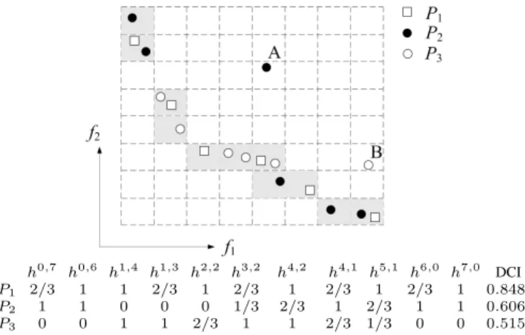
As an illustration to the calculation procedure of the DCI, Fig. 4 shows three Pareto front approximationsP1,P2, andP3 for a bi-objective problem. First,P1,P2, andP3 are put into the grid environment, and then 11 hyperboxes (marked in gray) are determined (here, solutionsAandB’s hyperboxes are not considered since they are dominated solutions in the mixed set). Afterward, for each of these hyperboxes, the contribution degree of the three approximations is calculated according to Eq. (8). For example, considering hyperbox h0,7 (0 and 7 correspond to its coordinates inf1 and f2, respectively), the contribution degree ofP2reaches 1 sinceP2 has a solution in this hyperbox; the contribution degree ofP1is1−12/3 = 2/3 as D(P1, h0,7) = 1; for approximation P3, the contribution degree is equal to zero because the distance fromP3toh0,7is farther than the threshold (D(P3, h0,7) =
√
10>√3). Finally, the average contribution degree of each approximation to these hyperboxes is obtained according to Algorithm 1 (line 10), and the DCI values ofP1,P2, andP3are 0.848, 0.606, and 0.515, respectively.
C. Time Requirement of DCI
The computational cost of DCI can mainly be divided into three parts. The first involves the operations of calculating
(a)DCI = 0.8000 (b)DCI = 0.7816 (c)DCI = 0.7026 (d)DCI = 0.4026
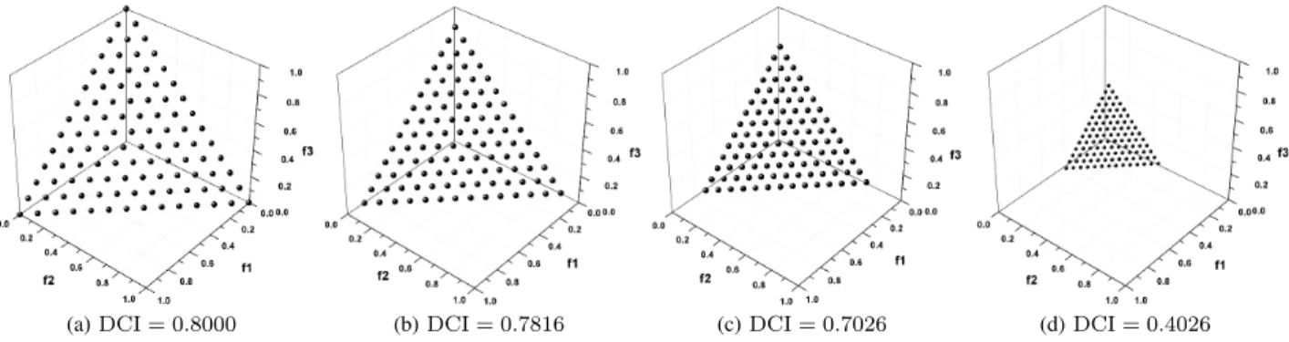
Fig. 5. DCI test for a group of artificial Pareto front approximations with different distribution ranges. All solutions in the approximations are located on the Pareto frontf1+f2+f3= 1.
the grid coordinates for the solutions in all approximations, which requires O(mLN) computations for an m-objective problem, whereL denotes the number of approximations and
N is the approximation size. The second part is related to the identification of nondominated solutions in the mixed set and to the record of their hyperboxes in grid, which requiresO(m(LN)2)comparisons. Clearly, the number of the considered hyperboxes, denoted as S, is not larger thanLN. The third part corresponds to the operation of calculating the contribution degree of all approximations to theShyperboxes. This requires O(mLN S) computations since at most mLN
comparisons are implemented for one hyperbox.
From the above analysis, the total complexity of the DCI ismax(O(m(LN)2), O(mLN S)) =O(m(LN)2), sinceS≤ LN. This cost is fully determined by the number of objectives and the size summation of all approximations, and thus is independent of the grid division and does not increase with the number of hyperboxes.
IV. EXPERIMENTS ANDDISCUSSIONS
In this section, we verify the proposed DCI indicator. First, three groups of artificial Pareto front approximations are introduced to show the effectiveness of DCI in assessing the spread and uniformity of approximations. Then, seven groups of Pareto front approximations obtained by six multiobjective optimizers in different numbers of objectives are used to further examine DCI, in view of their representative results in terms of diversity. Next, a comparison with two diversity indicators used widely in many-objective optimization is made analytically and empirically. Finally, the effect of the parame-ter (i.e., the grid division) in DCI is investigated, and a further discussion of the proposed indicator is made.
A. Artificial Examples
As mentioned before, diversity of Pareto front approxima-tions involves two facets, i.e., spread and uniformity. Here, we illustrate the validity of the proposed indicator by introducing several groups of artificial Pareto front approximations with different characteristics in spread and uniformity, with respect to a tri-objective optimization problem with a Pareto front
f1+f2+f3= 1 (0≤f1, f2, f3≤1).
Fig. 5 gives a group of artificial Pareto front approxima-tions. Each one has 105 solutions distributed uniformly on
the Pareto front of the problem. The only difference is their distribution range: the solutions in Fig. 5(a) are located over the whole Pareto front, and the solutions in other figures are located on a part of the Pareto front (from Fig. 5(b) to Fig. 5(d), the objective value of solutions belongs to the ranges [0.05,0.9], [0.1,0.8], and [0.2,0.6], respectively). Now, we apply the proposed indicator on these Pareto front approximations. The number of grid divisions is set to 19 for this and other tri-objective problems, unless otherwise stated. As can be seen from Fig. 5, the evaluation results given in the figure are consistent with the distribution range of the Pareto front approximations, which indicates that DCI can accurately reflect the spread of approximations.
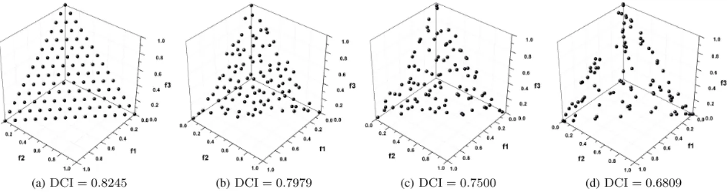
The Pareto front approximations in Fig. 6 are used to test the DCI in terms of distribution uniformity. The uniformity degree of four approximations is decreased gradually from Fig. 6(a) to Fig. 6(d), although all of them are located over the whole Pareto front. Clearly, the evaluation results show the effectiveness of DCI in assessing a set of approximations with different uniformity degrees. In addition, note that the same approximation in Fig. 5(a) and Fig. 6(a) has different DCI results since it has different competitors in the diversity comparison.
The above two groups of Pareto front approximations verify the correctness of the DCI in evaluating spread and uniformity separately. However, a comprehensive evaluation on a group of Pareto front approximations with different distribution ranges and uniformity degrees is necessary to further test the DCI; e.g., for two approximations, how to compare their diversity, if one performs better in terms of spread and the other has an advantage in uniformity. Fig. 7 shows this case. A group of Pareto front approximations are formed by copying the approximations in Figs. 5 and 6 (i.e., Fig. 7(a) = Fig. 6(c), Fig. 7(b) = Fig. 5(c), Fig. 7(c) = Fig. 6(d), and Fig. 7(d) = Fig. 5(d)). From the evaluation results in the figure, DCI could be considered as a tradeoff evaluation between spread and uniformity. An approximation with a great advantage over its competitors at one point will achieve a better DCI value, even though it performs slightly worse at the other point.
B. Real Examples
In this section, we apply the proposed indicator on Pareto front approximations obtained by six established
multiobjec-(a)DCI = 0.8245 (b)DCI = 0.7979 (c)DCI = 0.7500 (d)DCI = 0.6809
Fig. 6. DCI test for a group of artificial Pareto front approximations with different uniformity degrees. All solutions in the approximations are located on the Pareto frontf1+f2+f3= 1.
(a)DCI = 0.7463 (b)DCI = 0.6970 (c)DCI = 0.6329 (d)DCI = 0.4377
Fig. 7. DCI test for a group of artificial Pareto front approximations with different distribution ranges and uniformity degrees. All solutions in the approximations are located on the Pareto frontf1+f2+f3= 1.
tive optimizers, which are described as follows.
• Nondominated Sorting Genetic Algorithm II (NSGA-II) [58]. This is one of the most popular evolutionary multiobjective optimization (EMO) algorithms in the lit-erature. The main characteristics of NSGA-II are fast non-dominated sorting and crowding distance-based density estimation in fitness assignment.
• Average Ranking (AR) [70]. AR is regarded as a good alternative to rank solutions in a multiobjective population. It compares all solutions in each objective and independently ranks them, and the final rank of a solution is obtained by summing its ranks of all objectives. AR is found to perform successfully in searching towards the optimal direction for many-objective optimization problems [14], [17], although often converging into a subset of the Pareto front due to the lack of diversity maintenance schemes [17], [67].
• Indicator-Based Evolutionary Algorithm (IBEA)[71]. IBEA, introduced by Zitzler and K¨uenzli, aims to inte-grate the preference information of the decision maker into the multiobjective search. The main idea is to first define the optimization goal in terms of a binary per-formance measure and then directly use this measure in the mating and environmental selection processes. Since the single measure that involves both convergence and diversity is used to optimize a desired property of an approximation, IBEA is competitive with classic EMO algorithms in many-objective optimization [33].
• Diversity Management Operator (DMO)[51]. DMO is
a methodology to manage the use of diversity preserva-tion operators in dealing with many-objective problems. It adaptively tunes the diversity operator according to the requirement of the evolutionary population. If the diversity result is smaller than 1 by the Maximum Spread test [49], a specified diversity promotion mechanism is activated; otherwise, deactivated. Specifically in [51], DMO is implemented in NSGA-II and the crowding dis-tance is regarded as the diversity promotion mechanism.
• Territory Defining Evolutionary Algorithm (TDEA)
[72]. TDEA is a steady-state algorithm based on the concept of territory. Keeping the Pareto dominance re-lation in mind, the algorithm defines a territory around each solution and forbids other solutions to reside in it, thereby providing a good tradeoff between convergence and diversity.
• Average Ranking combined with Grid (AR+Grid)
[67]. AR+Grid is a hybrid method which uses grid to enhance diversity for AR in many-objective optimization. In AR+Grid, the AR strategy is employed to provide the selection pressure searching towards the Pareto front, and grid instrument is introduced to prevent solutions from being crowded in the objective space.
All tested multiobjective optimizers are given real-valued decision variables. A crossover probability pc = 1.0 and a
mutation probability pm = 1/l (where l is the number of
decision variables) are used. Simulated binary crossover (SBX) and polynomial mutation are separately chosen as crossover and mutation operators [3]. Both of them use the distribution
TABLE II
SETTINGS OF PARAMETERSτANDdINTDEAANDAR+GRID
Number of Objectives 3 4 5 6 8 10
τ 0.10 0.22 0.34 0.44 0.67 0.86
d 20 17 15 13 13 13
TABLE III
PARAMETER SETTINGS OFDCI
Number of Objectives 3 4 5 6 8 10
div 19 11 10 8 6 5
TABLE IV
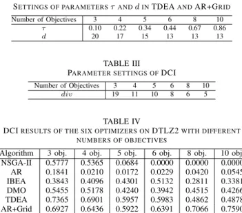
DCIRESULTS OF THE SIX OPTIMIZERS ONDTLZ2WITH DIFFERENT NUMBERS OF OBJECTIVES
Algorithm 3 obj. 4 obj. 5 obj. 6 obj. 8 obj. 10 obj. NSGA-II 0.5777 0.5365 0.0684 0.0000 0.0000 0.0000 AR 0.1841 0.0210 0.0172 0.0229 0.0420 0.0545 IBEA 0.3843 0.4096 0.4301 0.5132 0.2811 0.3381 DMO 0.5455 0.5178 0.4240 0.3942 0.4515 0.4266 TDEA 0.7365 0.6901 0.5957 0.5983 0.4862 0.4878 AR+Grid 0.6927 0.6436 0.5922 0.6391 0.7066 0.7590
indexes 20 (i.e., ηc = 20and ηm= 20). For each optimizer,
a population3 of 100 individuals and a predefined number
of 30,000 evaluations are set. Additionally, for TDEA and AR+Grid, two parameters τ and d (i.e., the size of territory in TDEA and the number of grid divisions in AR+Grid) are required respectively. They are given in Table II.
To verify the proposed indicator, two scalable test function DTLZ2 and DTLZ7 [20] are used. The Pareto front of DTLZ2 corresponds to the positive part of the unit hypersphere, and the Pareto front of DTLZ7 consists of 2m−1 disconnected regions. The total number of decision variables in the functions is l=m+n−1, wheremdenotes the number of objectives and n, set by users, is a parameter specifying the distance from solutions to the Pareto front. According to [20], here n
is set to 10 and 20 for DTLZ2 and DTLZ7, respectively. In the proposed DCI, a parameter div (i.e., the number of grid divisions) is required to divide the considered region into many hyperboxes. In this section, the setting of div is fixed and shown in Table III. A detailed investigation about different configurations of div will be given in Section IV-D.
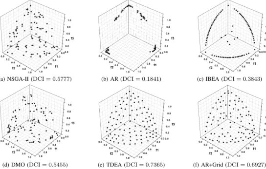
Table IV gives the diversity comparison results of the Pareto front approximations obtained by the six optimizers for different numbers (3, 4, 5, 6, 8, and 10) of objectives of DTLZ2. Due to the space limitation, only the distributions of the approximations for 3-,6-, and 10-objective problems are plotted in Fig. 8 to Fig. 10, respectively.
Fig. 8 shows the six Pareto front approximations with three objectives. Clearly, the optimizer TDEA performs the best: the solutions are uniformly located over the whole Pareto front. AR+Grid takes the second place, with its solutions distributed widely but not so uniformly as those of TDEA. The solutions obtained by NSGA-II and DMO are similar and distributed into many clusters on the Pareto front. The only difference between them is that the former seems to achieve a better result in terms of spread. The solutions of IBEA are of great regularity: most of them are located orderly on the boundary
3The archive set is also maintained with the same size if required.
of the Pareto front, but the rest of the region is populated sparsely. Due to the lack of a diversity maintenance method, the optimizer AR performs the worst among the selected opti-mizers, with the solutions concentrating around three scattered extreme points, i.e., (1,0,0), (0,1,0), and (0,0,1), of the Pareto front. Clearly, from the results in Fig. 8, it is clear that DCI is able to accurately reflect the relative distribution of Pareto front approximations: an approximation with a higher DCI value means that it performs better regarding the tradeoff between spread and uniformity.
The Pareto front approximations of the six optimizers for the six-objective DTLZ2 are plotted by parallel coordinates in Fig. 9. As seen in the figure, the distribution of these ap-proximations is consistent with the DCI results. The solutions obtained by NSGA-II fail to approach the Pareto front. In this case, none of them are located into the grid environment set by Eqs. (2) and (3), and thus the DCI value is assigned zero. The solutions of AR reach the optimal front, but nearly converge into a point. Although DMO performs significantly better than AR, its solutions do not appear to be well distributed over the whole Pareto front: most of them are grouped into many clusters, and some regions are lack of solutions. The rest three optimizers IBEA, TDEA, and AR+Grid perform better in terms of diversity maintenance, thereby producing higher DCI values. More specifically, IBEA, similar to the tri-objective case, prefers to converge into the boundary of the Pareto front, and only several solutions are obtained in other parts of the front. AR+Grid tends to be the most successful in maintaining diversity: its solutions have a better coverage of the optimal front than those of the other five optimizers.
Concerning the ten-objective case shown in Fig. 10, the distribution of the approximations is generally similar to that for the six-objective case. An interesting difference is that IBEA fails to find the whole Pareto front of the problem. In this case, DMO achieves a higher DCI value than IBEA. In addition, AR+Grid seems to show more advantage over TDEA in terms of diversity, and thus the difference between their DCI values is larger.
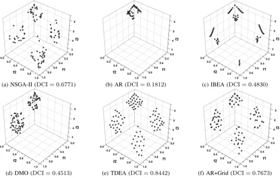
The above experiments have demonstrated the effectiveness of DCI on the problems with a linear or concave Pareto front. We now further examine its effectiveness when working on problems with other Pareto geometries. The test problem DTLZ7 has a disconnect Pareto front consisting of 2m−1 regions with both convex and concave shapes (where m
denotes the number of objectives), and is used to test an algorithm’s ability to maintain subpopulations in disconnected portions of the objective space.
Fig. 11 shows the Pareto front approximations obtained by one typical run of the six algorithms on the tri-objective DTLZ7. As can be seen from the figure, AR and DMO fail to find all the four Pareto optimal regions. The solutions of AR concentrate in the top region and the solutions of DMO are distributed in the top and left ones. Despite having found all the four regions, IBEA struggles to develop extensity, with most of the solutions located on the boundary of the regions. NSGA-II, TDEA, and AR+Grid perform similarly in terms of extensity, but differently in terms of uniformity. The solutions of TDEA have the best distribution uniformity,
(a) NSGA-II (DCI = 0.5777) (b) AR (DCI = 0.1841) (c) IBEA (DCI = 0.3843)
(d) DMO (DCI = 0.5455) (e) TDEA (DCI = 0.7365) (f) AR+Grid (DCI = 0.6927) Fig. 8. Pareto front approximations of the six algorithms and their DCI result on the tri-objective DTLZ2.
(a) NSGA-II (DCI = 0) (b) AR (DCI = 0.0229) (c) IBEA (DCI = 0.5132)
(d) DMO (DCI = 0.3942) (e) TDEA (DCI = 0.5983) (f) AR+Grid (DCI = 0.6391) Fig. 9. Pareto front approximations of the six algorithms and their DCI value on the six-objective DTLZ2 shown by parallel coordinates.
followed by those of AR+Grid and NSGA-II. Clearly, the assessment results of DCI confirm the above observations: an approximation with a higher DCI value means that it performs better regarding the comprehensive performance in finding multiple Pareto optimal regions as well as maintaining solutions’ uniformity and extensity in each region.
C. Comparative Study
This section is devoted to comparing DCI with other di-versity indicators. Here, two indicators, i.e., DM [30] and Maximum Spread (MS) [51], which are used widely in many-objective optimization [32], [51], [66], [67], are chosen as the peers. DM, as briefly described before in Section II, is a grid-based indicator that can reflect the spread and uniformity of
a Pareto front approximation. It takes the value in the range
[0,1]. The larger the value, the better the diversity.
MS, originally presented in [49], measures the length of the diagonal of the hypercube formed by the extreme objective values in a Pareto front approximation. Since the original indicator can be influenced heavily by the convergence of the considered approximation, Adra and Fleming [51] improved the MS indicator by considering the extreme values of the Pareto front as follows:
MS(P) = v u u t∑m k=1 (max p∈P(pk)−minp∈P(pk)) 2 /vu u t∑m k=1 (npk−ipk)2 (9)
(a) NSGA-II (DCI = 0) (b) AR (DCI = 0.0545) (c) IBEA (DCI = 0.3381)
(d) DMO (DCI = 0.4266) (e) TDEA (DCI = 0.4878) (f) AR+Grid (DCI = 0.7590) Fig. 10. Pareto front approximations of the six algorithms and their DCI value on the ten-objective DTLZ2 shown by parallel coordinates.
(a) NSGA-II (DCI = 0.6771) (b) AR (DCI = 0.1812) (c) IBEA (DCI = 0.4830)
(d) DMO (DCI = 0.4513) (e) TDEA (DCI = 0.8442) (f) AR+Grid (DCI = 0.7673) Fig. 11. Pareto front approximations of the six algorithms and their DCI result on the tri-objective DTLZ7.
value of individual p in the kth objective, and ipk and npk
denote the value of the ideal point and Nadir point in thekth objective, respectively.
The MS value of an approximation P close to one (i.e., MS(P) = 1) is desired. The value smaller than one (i.e., MS(P)<1) implies a lack of diversity ofP compared with the ideal result, which is most likely due to it converging into a sub-region of the Pareto front. The value larger than one (i.e., MS(P) > 1) indicates that P is located far away from the Pareto front. In the light of the above properties, MS is used to not only compare the distribution range of approximations but also guide the search in many-objective optimization [51]. First, we compare DCI with DM. Here, we focus on the accuracy of the assessment result for the two indicators.
Therefore, their other differences (e.g., in DM each hyperbox in grid needs to be accessed and a reference set is also required; see items 27 and 28 in Table I) are not considered. In DM, the setting of a hyperbox’s neighborhood is crucial for the assessment result. Two hyperboxes are called as neighbors to each other if the Manhattan distance of their grid coordinates is not larger than one. However, this setting, when the number of objectives of a problem is large, may cause an inaccurate estimation of the position of individuals, further leading to an inaccurate assessment of approximations’ diversity.
Let us consider a five-objective example with three hyper-boxesh1(0,0,0,0,0),h2(0,0,0,0,2), andh3(1,1,1,1,1). In DM, h3, rather than h2, is a neighbor of h1. Without loss
f2 f1 Pareto front P1 P2 P3 2 0 10 8 6 0 4 12 14 16 12 8 6 4 2 10
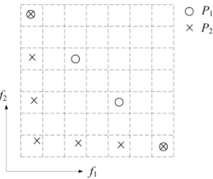
Fig. 12. An example of distribution of approximations for the MS and DCI indicators. MS(P1) =MS(P2) =MS(P3) = 1, and DCI(P1) = 12/15> DCI(P2) = 11/15>DCI(P3) = 7/15(div= 5).
of generality, let individuals A, B, and C be located in the center of hyperboxes h1, h2, and h3, respectively. Clearly, the Euclidean distance between B andA is shorter than that between C andA (2<√5), but only individual C is in the neighborhood ofA.
Let there be two approximations P and Q, with P con-sisting of A and B and Q consisting of A and C. In this case, DM(P) > DM(Q) because the distance between A
and B is mistakenly considered farther than that between
A and C, in view of the location of A and B in different neighborhoods in DM. However, as to the proposed DCI indicator, the distance between individuals is calculated based on the Euclidean distance of their grid coordinates. Therefore, DCI(P) = (CD(P, h1) +CD(P, h2) +CD(P, h3))/3 =
(1 + 1 + 1/6)/3 = 13/18 < DCI(Q) = (CD(Q, h1) +
CD(Q, h2) +CD(Q, h3))/3 = (1 + 1/3 + 1)/3 = 14/18. Next, we consider the MS indicator. Since MS only tests the range comparison between an approximation and the problem’s Pareto front, it may fail to assess the uniformity of solutions in the approximation. Moreover, even if testing the distribution range, MS may also give an inaccurate estimation because a poorly-converged approximation often has a broad range.
As an explanation to the problems of MS, Fig. 12 shows three approximations P1 = {(0,10),(5,5),(10,0)}, P2 =
{(0,10),(2,8),(10,0)}, and P3 = {(3,7),(15,5.5),(17,5)} for a bi-objective optimization problem with a Pareto front
f1 +f2 = 10. Clearly, P1 outperforms P2 in terms of diversity, and two individuals in P3 fail to approach the Pareto front. However, all the three approximations have the ideal MS result, i.e., MS(P1) = MS(P2) = MS(P3) = 1. Concerning the DCI indicator, the two individuals in P3 will be removed since they are dominated by some individuals in P1 andP2. The DCI results of three approximations are: DCI(P1) = 12/15>DCI(P2) = 11/15>DCI(P3) = 7/15.
2 3 4 5 6 7 8 9 10 0.0 0.2 0.4 0.6 0.8 1.0 Number of divisions D C I NSGA-II AR IBEA DMO TDEA AR+Grid
Fig. 13. DCI against the number of divisions of the six optimizers on the ten-objective DTLZ2.
TABLE V
DCIRESULTS OF THE SIX OPTIMIZERS ON THE10-OBJECTIVEDTLZ2 WITH DIFFERENT NUMBERS OF DIVISIONS(div). THE RESULTS ARE UNDERLINED WHEN THEY CAN CORRECTLY REFLECT THE DISTRIBUTION
DIFFERENCES AMONG THE OPTIMIZERS
div 2 3 4 5 6 7 8 9 10 NSGA-II 0 0 0 0 0 0 0 0 0 AR 0.766 0.353 0.109 0.055 0.036 0.023 0.012 0 0 IBEA 0.860 0.686 0.467 0.338 0.278 0.257 0.250 0.230 0.219 DMO 0.946 0.845 0.661 0.427 0.300 0.229 0.210 0.200 0.193 TDEA 0.977 0.885 0.739 0.488 0.320 0.212 0.180 0.175 0.169 AR+Grid 0.977 0.925 0.854 0.759 0.682 0.645 0.618 0.578 0.565
D. Study of Different Configurations of the Parameterdiv
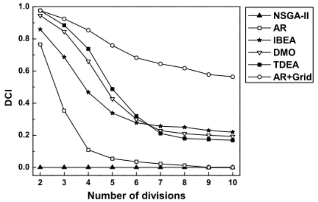
In DCI, a parameter div (the number of divisions) is required to divide the grid environment. Obviously, it largely affects the evaluation results since it determines the hyperbox location where Pareto front approximations are distributed. In this section, we investigate the effect of div and try to find an appropriate setting for a given problem. Here, we only show the results on a ten-objective problem due to the space limitation. Similar results can be obtained for problems with other numbers of objectives.
Fig. 13 plots the curves of the DCI results against the number of divisions for the six optimizers; they are also summarized in Table V for clarity. Clearly, there are two properties about the influence of div on the DCI. The first one is that the DCI value, in general, degrades with the growth of div. This is because the number of non-empty hyperboxes in grid increases with div, and for an approximation, more hyperboxes that are occupied by other approximations are needed to be considered. The second property is that within a certain range (div ∈ [3,5]), DCI can correctly compare the distributions of the approximations. Although the DCI values of the three competitive optimizers (i.e., IBEA, DMO, and TDEA) are all decreased, their differences remain mostly unchanged when div ∈ [3,5]. This provides an effective evaluation for the distributions of the approximations. On the other hand, when div is equal to 2, the DCI differences between TDEA and AR+Grid are too slight to reflect the distributions; and when div becomes larger than 6, the DCI values among IBEA, DMO, and TDEA may result in an incorrect judgment on their distributions. This occurrence may
be attributed to the following reason: a very smalldiv makes many solutions located in a hyperbox no matter how they are distributed; a largedivcauses that there are no other solutions existed in the neighborhood of a solution, which decreases the sensitivity of DCI to the extensity of approximations.
Intuitively, the optimal setting of div is the minimum required number of divisions of satisfying the condition that for a Pareto front approximation with ideal distribution (i.e., its individuals distributed uniformly over the whole Pareto front), the neighborhood4 of each individual does not contain any other individuals. This means that, ideally, the hyperboxes, in the dimensionality of the Pareto front of a given problem (i.e., the dimensionality of the manifold of Pareto optimal solutions in the objective space), should exactly cover all individuals so that no individual is located in the neighborhood of others. Namely,
divn=V(n,R)×N (10) whereV(n,R), representing the volume of a hyperbox’s neigh-borhood in the dimensionality of the Pareto front, denotes the volume of an n-dimensional hypersphere with radius R,
n denotes the dimensionality of the Pareto front, m denotes the number of objectives (obviously, n ≤m−1), and N is the size of the approximation. Here, R = √m+ 1/2, since two hyperboxes contribute nothing to each other (i.e, are non-neighboring) when their grid distance is larger than (or equal to)√m+ 1 (cf. Eq. (8)).
However, the optimal setting of div according to Eq. (10) may be infeasible in practice due to two reasons: 1) In DCI the neighborhood of a hyperbox corresponds to a hypersphere rather than a hypercube constructed by a set of hyperboxes, and 2) The shape of the Pareto front can be distinct for different problems, even if they have the same dimensionality. Considering a bi-objective problem with one-dimensional manifold of the Pareto front, the closest grid distance between two non-neighboring individuals is√m+ 1 =√2 + 1 =√3. However, in the 2-dimensional objective space, there are not two hyperboxes whose grid distance is equal to √3(the grid distance between two hyperboxes∈ {1,√2,2,√5,2√2,3...}). In addition, approximations with different Pareto front shapes may require different numbers of hyperboxes. Fig. 14 gives a 2-objective example regarding two approximations, one (P1) with a straight line Pareto front and the other (P2) with a folding line Pareto front. Clearly, 49 hyperboxes can contain only 4 uniformly-distributed non-neighboring individuals from
P1 but 7 ones from P2. This means that P1 requires more hyperboxes than P2 when they have the same number of individuals.
In view of these reasons, we givediva rough range estima-tion rather than a precise value. On the one hand, according to Eq. (10),div= (V(n,√m+1/2)N)1/n>(V
(n,√m/2)N)1/n. On the other hand, as mentioned before, sometimes there are no two hyperboxes whose grid distance is equal to the ideal grid distance (√m+ 1). In this case, the radius of a hyperbox’s neighborhood is larger than√m+ 1/2. For instance, for a 2-objective problem (e.g., the example in Fig. 14), the radius of 4Here, the neighborhood of an individual means the neighborhood of the hyperbox where the individual is located.
Fig. 14. An example of approximations with different Pareto front shapes requiring different numbers of hyperboxes.
the hyperbox’s neighborhood will be1,√5/2, or√2. In fact, under the condition of having the same number of individuals, an approximation with the 45◦ hyperplane shape (like P1 in Fig. 14) requires the most hyperboxes. In this case, the radius of the hyperbox’s neighborhood will be equal to√m. Consequently,div≤(V(n,√m)N)1/n.
Moreover, sincedivmust be an integer and the total number of hyperboxes should be larger than (or equal to) that of hyperboxes occupied by individuals and their corresponding neighborhoods, therefore we have
⌈(V(n,R1)N) 1/n⌉ ≤div≤ ⌈(V (n,R2)N) 1/n⌉ (11) where R1 = √ m/2 and R2 = √ m. For an n-dimensional hypersphere, its volume V(n,R) can be calculated by the following formula: V(n,R)= { (πk/k! )Rn, for n= 2k ( 22k+1k!πk/(2k+ 1)! )Rn, for n= 2k+ 1 (12) wherekis an integer larger than or equal to zero. Taking the 4-objective DTLZ2 as an example, heren= 3,R1= 1andR2=
2. So, V(n,R) = 43πR3, div ∈ [⌈(43πN) 1/3 ⌉,⌈(32 3πN) 1/3 ⌉], and further div is in the range[8,15]if N= 100.
Although the effectiveness of DCI seems to be insensitive to div in a certain range, different div settings will prefer different distributions of Pareto front approximations in the context of spread and uniformity. Next, we give two examples to explain this fact. Figs. 15 and 16 show two groups of Pareto front approximations obtained by AR+Grid with different parameter settings on the 3- and 4-objective DTLZ2; the DCI results for different div settings are also included in the figures. Clearly, the solutions in Figs. 15(a) and 16(a) are located extensively but non-uniformly since they concentrate (or even coincide) in a number of scattered regions; whereas the solutions in Figs. 15(c) and 16(c) are uniformly distributed (i.e., adjacent solutions have basically equal spacing) but fail to cover the whole Pareto front.
An interesting observation from the comparison betweenP1 andP3 in the figures is that with a smalldiv, an extensively-distributed approximation has a better DCI value, while with a largediv, a uniformly-distributed approximation is preferred. This phenomenon is mainly due to the sensitivity of DCI to the number of hyperboxes in grid. A smalldivmakes hyperboxes decreased in number; an extensively-distributed approximation
(a)P1(d= 14) (b)P2(d= 20) (c)P3(d= 28)
div 12 14 16 17 18 19 20 21 23 25
DCI(P1) 0.8420 0.7809 0.7463 0.7353 0.7188 0.6893 0.6559 0.6278 0.5887 0.5710 DCI(P2) 0.8620 0.8315 0.7958 0.7946 0.7704 0.7535 0.7369 0.7059 0.6860 0.6600 DCI(P3) 0.7561 0.7416 0.7030 0.6985 0.6967 0.6799 0.6714 0.6697 0.6553 0.6335
Fig. 15. Investigation of different numbers of divisions (div) in DCI for the tri-objective DTLZ2. The Pareto front approximationsP1,P2, andP3obtained by AR+Grid with different parameter settings.
(a)P1(d= 9) (b)P2(d= 17) (c)P3(d= 30)
div 8 9 10 11 12 13 14 15
DCI(P1) 0.7956 0.7255 0.6792 0.6360 0.5902 0.5398 0.5256 0.4833 DCI(P2) 0.8656 0.8436 0.8203 0.7899 0.7625 0.7307 0.6812 0.6558 DCI(P3) 0.7169 0.6649 0.6473 0.6350 0.6259 0.5991 0.5940 0.5858
Fig. 16. Investigation of different numbers of divisions (div) in DCI for the four-objective DTLZ2. The Pareto front approximationsP1,P2, andP3obtained by AR+Grid with different parameter settings.
will cover (or at least be not far away from) any considered hyperbox, thereby obtaining a relatively higher average con-tribution degree. On the other hand, whendivbecomes larger, the number of hyperboxes increases, and correspondingly the grid distance between solutions becomes longer; the solutions that are uniformly distributed and are away from each other with certain distance will have a higher likelihood in different hyperbox neighborhoods, thereby providing relatively higher contributions to the evaluation result.
The above properties can make the setting of div in the DCI consistent with the preference of the user. In the absence of guidance information, the optimal setting, if attainable, is first suggested (e.g.,div= 19for a 3-objective problem with a 2-dimensional manifold of Pareto front when the size of approximations is equal to 100); otherwise, a value around the median of the range in Eq. (11) can be replaced. On the other hand, a slightly lower (or higher) div is recommended if the user prefers an extensive (or uniform) distribution of the solutions in Pareto front approximations.
E. Discussion
None of performance indicators can assess all kinds of distributions of approximations in the area. Like existing diversity indicators, DCI also fails to deal with some specific distributions. Since DCI considers relative positions of two
(several) approximations in a grid, it may not be able to distinguish approximations with similar (or same) relative positions in the grid but different distributions in the objective space. This is a weakness of the proposed indicator, which will be one important issue for our future study. A possible way to cope with this problem may be to assign different weights to the considered hyperboxes according to their distributions in the objective space.
In addition, DCI does not consider the difference between individuals in the same hyperbox. This can affect the accuracy of the assessment result to some extent. A refined division of grid (i.e., a largediv) can reduce the probability of individuals located in same hyperboxes, but it decreases the sensitivity of DCI to the extensity of approximations, as explained in the previous section.
Here, it is worth mentioning that DCI only fails to assess several approximations which are located in the exactly same set of hyperboxes. In most cases, DCI can reflect the in-formation regarding several approximations where there exist individuals distributed in the same hyperboxes. For example, considering two approximations P and Q with the same number of individuals, ifP has more individuals in the same hyperboxes than Q, in general P will obtain a poorer DCI value since it provides fewer hyperboxes to be considered in the DCI calculation.