COMPUTATIONAL HYPERSONIC BOUNDARY-LAYER STABILITY AND THE VALIDATION AND VERIFICATION OF EPIC
A Dissertation by
TRAVIS SCOTT KOCIAN
Submitted to the Office of Graduate and Professional Studies of Texas A&M University
in partial fulfillment of the requirements for the degree of DOCTOR OF PHILOSOPHY
Chair of Committee, Helen L. Reed Committee Members, Rodney Bowersox
Edward White Prabir Daripa Head of Department, Rodney Bowersox
May 2018
Major Subject: Aerospace Engineering
ABSTRACT
Laminar-to-turbulent transition is a process that is critical in determining the system drag and surface heating of a flight vehicle, and the ability to predict, and possibly control, this process has become an essential component in vehicle design. The linear and nonlinear parabolized stability equations provide a method of analyzing different regions of the flowfield around a vehicle in a way that is both efficient and accurate. These methods have continued to evolve in terms of both capability and robustness. Coupled with data from wind tunnel experiments, they provide a powerful tool in understanding and addressing flow phenomena involved in the process of laminar-to-turbulent transition.
EPIC is a parabolized stability equations (PSE) solver developed within the Computa-tional Stability and Transition laboratory at Texas A&M University that can address both the linear and nonlinear aspects of the stability problem. This capability provides a means to evaluate different instabilities and the underlying physics that drives them. PSE results are computed for several hypersonic geometries including the Langley 93-10 cone, Purdue compression cone, yawed straight cone, and HIFiRE-5 elliptic cone. Disturbances that are both two-dimensional and three-dimensional in nature are analyzed and compared with re-sults obtained from direct numerical simulations, wind tunnel experiments, and alternate PSE codes. In addition, techniques for modeling stationary crossflow vortex paths and the evolution of spanwise wavenumber from the basic-state solution are formulated.
ACKNOWLEDGMENTS
I am extremely grateful to have had the opportunity to interact and work with the many individuals that have helped guide me during my studies at Texas A&M. I know that the present work was only made possible because of the contributions and support of those around me.
First and foremost, I would like thank my advisor, Dr. Helen Reed, for giving me the opportunity to pursue my graduate degree. I have gained far more than I can describe from her never-ending guidance, encouragement, and support. I could not imagine having a graduate experience with a better professor or person.
I am very appreciative for the discussions I have had with Dr. Rodney Bowersox, Dr. William Saric, and both of their experimental groups. I was able to draw from their vast knowledge and experience in order gain a perspective that I would not have achieved from solely a com-putational viewpoint. Ian Neel, Jerrod Hofferth, and Alex Craig deserve a special thanks for their direct contributions to this study. I would also like to acknowledge the other members of my committee, Dr. Edward White and Dr. Prabir Daripa, for their helpful advice and suggestions.
Thank you to my colleagues from the Computational Stability and Transition lab, Ed-uardo Perez, Matthew Tufts, Nicholas Oliviero, Alexander Moyes, Daniel Mullen, and Joseph Kuehl. I consider myself very fortunate to have been able to work with each of you on a daily basis and am grateful for both your support and friendship.
I would like to thank Rebecca Marianno and Colleen Leatherman for their tireless work. Their efforts have worked wonders towards providing an organized graduate experience, and our lab would not operate properly without them.
Finally, I would like to thank my family for their constant love and support. I would not be who I am today without you.
CONTRIBUTORS AND FUNDING SOURCES
Contributors
This work was supported by a dissertation committee consisting of my advisor Dr. Helen Reed and professors Dr. Rodney Bowersox, Dr. Edward White, and Dr. Prabir Daripa. Funding Sources
This graduate study was supported by Program Manager Ivett Leyva under AFOSR grant FA9550-14-1-0365, Program Managers John Schmisseur and Rengasamy Ponnappan in the Air Force/NASA National Hypersonics Science Center in Laminar-Turbulent Transition under grant FA9550-08-0308, and by a dissertation research fellowship from the Texas Space Grant Consortium.
NOMENCLATURE
A Disturbance Amplitude
A,B,C,D,E,F Linear Stability Matrices
c Disturbance Phase Speed
Cf Skin-Friction Coefficient
cp Specific Heat Capacity at Constant Pressure
cv Specific Heat Capacity at Constant Volume
d Straight Line Distance
F Frequency (kHz)
h1, h2, h3 Curvature Terms in (ξ, η, ζ)Directions, Respectively
i, j, k Basic-State Indices
kc Wavenumber (Number of Waves)
m Wavenumber Observed Locally (Number of Waves)
M Mach Number
N L Vector of Nonlinear Terms
Ny Number of Computational Normal Points
P Absolute Static Pressure
P r Prandtl Number
r Cylindrical Coordinate in Radial Direction
R Radius of Revolution
Rg Specific Gas Constant
Re Reynolds Number
Re′ Unit Reynolds Number
s Surface Distance
St Stanton Number
t Time
T Absolute Static Temperature
u, v, w Velocity Components in (ξ, η, ζ)Directions, Respectively
x, y, z Orthogonal Cartesian Coordinates
α Wavenumber in ξ Direction
β Wavenumber in ζ Direction
γ Ratio of Specific Heats
δ Boundary Layer Length Scale
ζ Spanwise Coordinate Tangent to Surface and
Perpendic-ular to Marching Direction ξ
η Wall-normal Coordinate and Perpendicular to Marching
Direction ξ
θ Cylindrical Coordinate in Azimuthal Direction
κ Thermal Conductivity
λ Wavelength
λL Lagrange Multiplier
λv Second Viscosity Coefficient
µ Dynamic Viscosity Coefficient
ξ Coordinate Along Marching Direction
ρ Density
ϕ Primitive Variable Vector (u, v, w,T, ρ)
χ Scale Factor
ψ Wave Angle
ACRONYMS
ACE Adjustable Contour Expansion
AoA Angle of Attack
AFRL Air Force Research Laboratory
BAM6QT Boeing/AFOSR Mach-6 Quiet Tunnel
CFD Computational Fluid Dynamics
CST Computational Stability and Transition
DNS Direct Numerical Simulation
DPLR Data Parallel Line Relaxation
DRE Discrete Roughness Element
DSTO Defense Science and Technology Organization
EPIC Euonymous Parabolized Instability Code
HIFiRE Hypersonic International Flight Research
Experimentation
LNS Linearized Navier-Stokes
LPSE Linear Parabolized Stability Equations
LST Linear Stability Theory
M6QT Mach 6 Quiet Tunnel
NPSE Nonlinear Parabolized Stability Equations
PSE Parabolized Stability Equations
RMS Root Mean Square
SUBSCRIPTS
art Artificial Value
e Quantity Evaluated at Edge of Boundary Layer
i Imaginary Value
ref Reference Value
w Quantity Evaluated at Wall
0 Initial Value
∞ Quantity Evaluated at Infinity
⊥ Perpendicular
ACCENTS
T Transpose
∧ Shape Function Quantity
† Complex Conjugate
− Basic State Quantity
◦ Degrees
′ Disturbance Quantity
∼ Slowly Varying
TABLE OF CONTENTS
Page
ABSTRACT . . . ii
ACKNOWLEDGMENTS . . . iii
CONTRIBUTORS AND FUNDING SOURCES . . . iv
NOMENCLATURE . . . v
TABLE OF CONTENTS . . . ix
LIST OF FIGURES . . . xii
LIST OF TABLES . . . xvi
1. INTRODUCTION AND BACKGROUND . . . 1
1.1 Motivation. . . 1
1.2 Objective . . . 3
1.3 Background on Instability Mechanisms . . . 3
1.4 Advancement of Stability Methods . . . 8
1.5 Outline . . . 11 2. STABILITY METHOD . . . 12 2.1 Governing Equations . . . 12 2.1.1 Viscosity. . . 13 2.2 Curvature . . . 13 2.3 Disturbance Equations . . . 14
2.3.1 Linear Stability Theory . . . 15
2.3.1.1 Eigenvalue Solution . . . 17
2.3.2 Linear Parabolized Stability Equations . . . 18
2.3.3 Nonlinear Parabolized Stability Equations . . . 20
2.4 EPIC. . . 23
3. BASIC-STATE DATA EXTRACTION . . . 24
3.1 Data Preparation . . . 25
3.2 Surface Proximity . . . 27
3.2.1 Flow Variable Acquisition . . . 28
3.2.3 Surface Curvature . . . 31
3.2.4 Stepping . . . 33
4. VARIATION OF SPANWISE WAVENUMBER . . . 35
5. PURDUE COMPRESSION CONE . . . 40
5.1 Geometry and Grid Topology . . . 40
5.1.1 Flow Conditions . . . 41
5.2 LPSE . . . 42
5.2.1 Convergence Study . . . 43
5.2.2 Influence of Boundary-Layer Height on Second Mode . . . 46
5.3 K-type Breakdown . . . 47
6. LANGLEY 93-10 FLARED CONE . . . 56
6.1 Geometry and Grid Topology . . . 56
6.1.1 Flow Conditions . . . 57
6.2 LPSE . . . 58
6.2.1 Influence of Boundary-Layer Height on Second Mode . . . 59
6.2.2 Effect of Wall Temperature . . . 61
6.2.3 Effect of Small Angle of Attack on Second Mode . . . 62
7. YAWED STRAIGHT CONE . . . 67
7.1 Geometry and Grid Topology . . . 67
7.1.1 Flow Conditions . . . 68
7.2 Windward and Leeward LPSE . . . 69
7.3 Vortex Paths and Spanwise Wavenumber Evolution . . . 70
7.4 3-D LPSE . . . 77
7.5 3-D NPSE . . . 81
7.5.1 Instability Mechanisms Observed at Braunschweig . . . 84
7.5.2 M6QT Experimental Comparison . . . 86
8. HIFiRE-5 ELLIPTIC CONE . . . 93
8.1 Geometry and Grid Topology . . . 93
8.1.1 Flow Conditions . . . 93
8.2 Linear Primary Instability Analysis . . . 95
8.2.1 2-D LPSE . . . 95
8.2.2 Stationary Crossflow . . . 96
8.2.2.1 Variation of Spanwise Wavenumber . . . 96
8.2.2.2 3-D LPSE . . . 97
8.2.3 Traveling Crossflow . . . 99
8.2.4 Spanwise Wavelength . . . 100
8.2.5 Convergence Study . . . 102
8.3.1 Amplitude Evaluation . . . 103
8.3.2 Flow Visualization and Reconstruction . . . 105
9. NOTABLE ADVANCEMENTS . . . 108
10. CONCLUSIONS AND FUTURE WORK . . . 110
10.1 Conclusions. . . 110
10.2 Future Considerations . . . 112
10.2.1 Additional DNS for Yawed Straight Cone . . . 112
10.2.2 Extended NPSE Validation . . . 113
10.2.3 Receptivity Model . . . 114
10.2.4 Low-Speed Flows . . . 114
REFERENCES . . . 115
APPENDIX A. MATHEMATICAL FORMULAS . . . 125
A.1 Winding Number . . . 125
A.2 General 2-D Interpolation . . . 126
A.3 Linear Least Squares . . . 128
APPENDIX B. LST MATRIX FORMULATION . . . 130
B.1 A-Matrix . . . 130
B.2 B-Matrix . . . 131
B.3 C-Matrix . . . 133
APPENDIX C. LPSE MATRIX FORMULATION . . . 141
C.1 A-Matrix . . . 141
C.2 B-Matrix . . . 142
C.3 C-Matrix . . . 142
C.4 D-Matrix . . . 145
LIST OF FIGURES
FIGURE Page
1.1 Diagrams of typical crossflow profiles . . . 7
3.1 Order for combination of basic-state datasets . . . 26
3.2 Projecting data points to common plane. . . 28
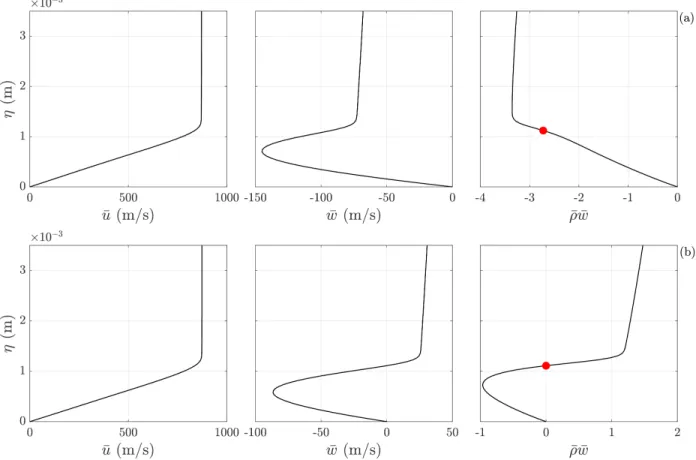
3.3 Basic-stateu, w, and ρw profiles (a) in the down-geometry direction and (b) oriented in the direction of marching along a stationary crossflow vortex path . 31 3.4 Method for finding surface curvature . . . 32
3.5 Flattened geometries for surface marching . . . 34
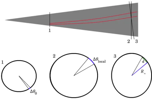
4.1 Visual portrayal of the formulation for the variation of wavenumber perpen-dicular to the marching path . . . 37
5.1 Purdue compression cone . . . 41
5.2 Purdue compression cone laminar basic-state solution . . . 41
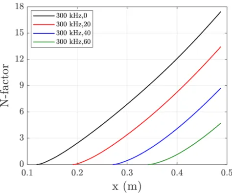
5.3 Second-mode N-factors on Purdue compression cone . . . 43
5.4 Görtler N-factors on Purdue compression cone . . . 44
5.5 Second-mode N-factors for three grid densities . . . 45
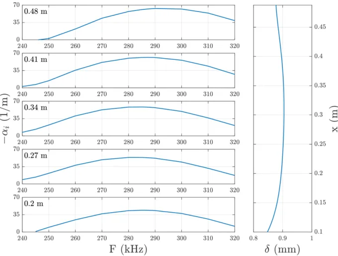
5.6 Local growth rates for LPSE second-mode instabilities and boundary-layer thickness of the Purdue compression cone . . . 46
5.7 N-factors for 2-D and oblique second-mode instabilities . . . 50
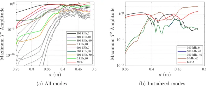
5.8 Maximumu-amplitudes from NPSE for K-type simulation . . . 51
5.9 MaximumT-amplitudes from NPSE for K-type simulation . . . 52
5.10 Stanton number distribution on the surface of the Purdue compression cone . . . 52
5.11 Time averaged skin-friction coefficients along axial slices of the Purdue com-pression cone . . . 54
6.1 Langley 93-10 flared cone . . . 56
6.2 Langley 93-10 laminar basic-state solution . . . 57
6.3 Comparison of ρu mass-flux mode shapes for locally most amplified LPSE frequencies and experimental fluctuating voltage profiles . . . 59
6.4 Second-mode N-factors with Tw = 398 K . . . 60
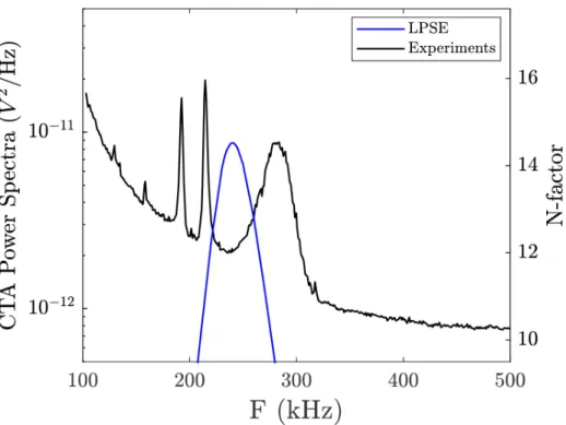
6.5 Peak frequencies of LPSE N-factor compared with RMS of experimental spec-tra atx= 0.5m . . . 61
6.6 Local growth rates for LPSE second-mode instabilities and boundary-layer thickness of the Langley 93-10 cone . . . 62
6.7 Wall temperature distributions for the Langley 93-10 flared cone. Shown are the experimental conditions in the M6QT, the adiabatic distribution, and two computational values with constant Tw. . . 63
6.8 Second-mode N-factors with Tw = 386 K . . . 64
6.9 Most amplified second-mode frequencies from computations and experiments. Black error bars indicate uncertainty in the laser-scan alignment technique. Red error bars provide a notional estimate of the effect of residual out-of-plane misalignment. . . 65
6.10 LPSE results for most unstable second-mode frequency for the Langley 93-10 cone at0.32◦ AoA along the windward plane and azimuthally off windward . . . 66
7.1 Structured grid for the yawed straight cone . . . 68
7.2 Grid topology on nose of yawed straight cone . . . 69
7.3 Yawed straight cone laminar basic-state solution. . . 70
7.4 2-D disturbance N-factors along the leeward plane . . . 71
7.5 Disturbance N-factors along the windward plane . . . 71
7.6 Comparison of inflection-point method (solid lines) vs. DNS vortex trajectories (dashed lines) for 5 paths . . . 72
7.7 Comparison of inflection-point method paths, DNS trajectories from Balaku-mar & Owens, and DNS trajectories from Gronvall et al. . . 73
7.8 Comparison of DNS vortex trajectories (red dots), mass-flux inflection-point paths (black lines), spanwise velocity inflection-point paths (green dashed lines), and inviscid streamlines (blue dashed lines) . . . 74
7.9 Comparison of inflection-point paths (black lines) and paths extracted from the Purdue experiment (red dashed lines) . . . 76 7.10 Varying azimuthal wavenumber for each path . . . 77 7.11 N-factors for stationary crossflow using (a) inflection-point paths and (b)
in-viscid streamlines. The “dot” marks an N-factor of11. The lower, center, and upper dashed lines on the flattened cone represent 30◦, 90◦, and 150◦ from windward, respectively. . . 78 7.12 N-factors for traveling crossflow using inviscid streamlines. The “dot” marks
an N-factor of 11. The lower, center, and upper dashed lines on the flattened cone represent30◦, 90◦, and 150◦ from windward, respectively. . . 79 7.13 Maximumu-amplitudes from NPSE (solid lines) compared withu-amplitudes
calculated from DNS (dashed lines) . . . 82 7.14 Total flow ofu-velocity (basic state combined with perturbation values)
show-ing the development of stationary crossflow vortices at axial locations of (a) 200 mm, (b) 175 mm, (c) 150 mm, and (d)100 mm . . . 83 7.15 (a) LPSE N-factors for frequencies between10−70kHz with a red line marking
x = 0.36 m and (b) N-factors at an axial location of 0.36 m with azimuthal angleθ = 70◦ from windward (maximum N-factor corresponds to33kHz and is shown with the vertical blue line) . . . 85 7.16 Wave angle based on local inviscid direction vs. frequency. The vertical blue
line marks the33 kHz disturbance. . . 86 7.17 u, v, and w mode shapes of disturbances at neutral points for (a) 0 kHz, (b)
10kHz, (c) 20 kHz, and (d) 33 kHz . . . 87 7.18 Growth rates for disturbances with constant wavenumber kc at x= 0.36m . . . . 88 7.19 (a) Inflection-point paths and (b) their varying azimuthal wavenumbers are
provided. Each× marks a location of comparison with experimental results. . . 89 7.20 (a) N-factors along a vortex path intersecting the experiment measurement
location at x = 0.37 m and (b) N-factor vs. number of waves predicted by equation 4.4 at the measurement location . . . 89 7.21 Development of stationary crossflow vortices at an azimuthal angle of 118◦
at x = 360 mm (top), 370 mm (center), and 380 mm (bottom) for NPSE computations (left) and the M6QT experiment (right). Contours are created using normalized ρu mass flux. (Experiment image attributed to Craig & Saric [1]) . . . 91
7.22 Comparison of computational and experimental RMS representing the mode shape of the disturbance. The lines correspond to locations at 118◦ from windward and axial distances of 360 mm (blue), 370 mm (red), and 380 mm
(green). (Experiment image attributed to Craig & Saric [1]). . . 92
8.1 Mach contours of the HIFiRE-5 geometry . . . 94
8.2 2-D N-factors at different frequencies along the attachment line . . . 95
8.3 2-D N-factors at different frequencies along the leeward plane . . . 96
8.4 Ratio variation of local azimuthal wavenumber along HIFiRE-5 geometry . . . 98
8.5 N-factors for stationary crossflow using (a) inflection-point paths and (b) in-viscid streamlines. The s = 0 location on the flattened cone represents the leeward plane. . . 98
8.6 N-factors for traveling crossflow using inviscid streamlines. Thes= 0location on the flattened cone represents the leeward plane. . . 99
8.7 Spanwise wavelengths for stationary crossflow disturbances along inflection-point paths using the global wavenumber kc which produced the largest N-factor for each. Paths pass through the region of highest amplification on the geometry and are compared with the average DNS wavelength. . . 101
8.8 Inflection-point paths for three grid resolutions of the HIFiRE-5 geometry. Global (y, z) coordinates were converted to θ for comparison where 90◦ rep-resents the attachment line along the semi-major axis. . . 103
8.9 Stationary crossflow N-factors for grid resolutions of 49, 96, and 193 million cells . . . 104
8.10 Maximum u-amplitudes from NPSE . . . 105
8.11 Total flow of ρu mass flux showing the development of stationary crossflow vortices at different axial locations and arc lengths (measured from leeward) of the cone. The axial locations in terms ofx/Lare (a)0.95, (b)0.9, (c)0.85, (d) 0.8, (e) 0.75, and (f) 0.7. The flow is from bottom to top. . . 106
LIST OF TABLES
TABLE Page
5.1 Inputs for K-type NPSE . . . 50 7.1 Comparison of various computational and experimental flow variables used in
the present analysis of the yawed straight cone . . . 68 7.2 Effects of spanwise curvature (h3) and wavelength scale factor (χ2) on
max-imum N-factor. The case marked with an asterisk (∗) does not satisfy the irrotationality condition. . . 80 7.3 Inputs for stationary crossflow NPSE . . . 81 8.1 Path designations, axial x locations (in meters), their arc length locations
(in meters) measured from the leeward plane, and the spanwise wavenumbers resulting in the largest LPSE N-factors for stationary crossflow . . . 97
1. INTRODUCTION AND BACKGROUND
1.1 Motivation
Modern research and development continues to focus on new and efficient ways to reduce system drag for aircraft designs. For example, the International Air Transport Association reported that commercial-class aircraft used 18.8% of the operating budget on fuel in 2017 [2]. This is a value that is on the order of billions of dollars, and improvements in vehicle performance can result in substantial savings.
System drag can be decomposed into separate components based on the source of the effect. For a high speed civil transport aircraft, Bushnell [3] states that the drag is approxi-mately on the order of 13 skin-friction drag, 13 wave drag, and 13 vortex drag due to lift. When flow separation occurs, another component deemed pressure drag also becomes a significant contributor. The process of boundary-layer transition heavily impacts drag and produces many other effects on the performance of an aircraft. In addition to reducing skin-friction drag, laminar flow also yields benefits in reducing the heating that occurs at the surface of a vehicle. This becomes even more important when one enters the hypersonic flow regime as turbulent flow can produce heating rates that are higher than those of laminar flow by a factor of six or more. In other instances, turbulent flow can be used as a beneficial tool in the design of an aircraft. One such example occurs at the inlet of a jet engine. Turbulent flow at this location will improve the mixing of the fuel and the oxidizer resulting in a higher efficiency. It can also prevent flow separation in areas that are susceptible under laminar flow conditions and help to maintain control authority for control surfaces. Additionally, preventing flow separation can reduce the penalties incurred by pressure drag in the aft re-gion of a body. Pressure drag from separation often carries a larger penalty than the increase in skin-friction drag due to turbulent flow.
progress in the field of hypersonics has led to the development and testing of investigative and flight capable vehicles. One such program was the DARPA/Air Force Falcon program [4]. The objectives of the program were to create a reusable vehicle that can take-off and land on modern runways, achieve hypersonic cruise velocities, and reach any location in the world in two hours or less. The test flight of the Hypersonic Technology Vehicle #2 (HTV-2) required a unique combination of integrated technologies. These included the development of lightweight high-temperature materials, optimization of aerodynamic design for high lift to drag ratio, and a sustained propulsion system. Two flights were conducted with the HTV-2 achieving speeds of Mach 20 for both. However, each was only able to sustain flight for approximately 9 minutes out of the 30 minutes designated for the mission before being terminated. It was reported that damage to the outer aeroshell due to the combination of aerodynamic force and heating contributed to this result.
Another program labeled the Hypersonic International Flight Research Experimentation (HIFiRE) program was a joint hypersonic flight test program by the Air Force Research Lab-oratory (AFRL) and the Australian Defense Science and Technology Organization (DSTO) [5]. The main objective was to obtain aerothermodynamic data including the heating cre-ated by a transitional boundary layer. HIFiRE-1 was the first of the flight test series and consisted of an axisymmetric circular cone geometry with a 7◦ half angle. The flight test launched in March 2010 and successfully provided transition measurements in a flight envi-ronment. Later flight tests were organized in order to study boundary layer stability and transition on a non-axisymmetric configuration. This geometry was a 2:1 elliptic cone and focused on leading edge transition and three-dimensional (3-D) instabilities. The first flight, HIFiRE-5a, was tested in April 2012, but did not obtain the intended trajectory or Mach number because the second stage of the sounding rocket failed to ignite. Despite this, useful supersonic data was still obtained. A second flight was completed in May 2016 and desig-nated HIFiRE-5b. This second flight successfully achieved hypersonic speeds and provided extensive data in regions associated with various disturbances including near the centerline,
on the leading edges, and in the highly 3-D region between them [6].
The results of these recent flight tests have spawned a number of studies showing that the development of instabilities in the boundary layer leading to transition to turbulence can create extreme levels of heating which could have devastating effects on a hypersonic vehicle. For this reason, it is vital to understand and predict the behavior of such mechanisms and any influence they might have on the vehicle flight capabilities.
1.2 Objective
This work uses the Euonymous Parabolized Instability Code (EPIC [7]) in combination with a basic-state data processing and extraction code, both developed within the Compu-tational Stability and Transition (CST) laboratory at Texas A&M University. The primary objective of the present work is to develop methods to accurately model the physics of vari-ous mechanisms and, by extension, the transition process for a variety of general hypersonic vehicles. As transition studies are known to be very sensitive, a very important aspect of this work is a close collaboration with high quality experiments providing both crucial validation and a different perspective in the identification of relevant mechanisms.
1.3 Background on Instability Mechanisms
The behavior of a laminar boundary layer exposed to freestream disturbances or surface imperfections is often determined by the growth of an assortment of different instability mechanisms. Much of the foundation and most extensive descriptions of the stability prob-lem are provided by Mack [8] and Federov [9] including an in depth analysis of supersonic boundary layers for speeds up to Mach 10, key differences between disturbances in the su-personic and subsonic regimes, laminar flow control, and receptivity.
Receptivity in particular is an elusive aspect that heavily influences the onset of transition [10, 11, 12, 13] and is the beginning stage for any stability analysis. Receptivity determines how freestream vorticity, freestream noise, and surface roughness affect the initial amplitude of a disturbance as it enters the boundary layer. A close collaboration between computations
and experiments is necessary in order to investigate this multivariable process. Computa-tions will require validation of receptivity models provided from experimental measurements. However, the measurements will have undergone a stage of receptivity as the disturbances enter the boundary layers of the measurement devices themselves, further adding to the complexity of the problem.
A combination of efforts from experiments, computations, and theory have revealed that hypersonic boundary layers are especially vulnerable to the following mechanisms:
1. Attachment-Line Instability 2. Leading-Edge Contamination 3. First Mode 4. Second Mode 5. Görtler Instability 6. Traveling Crossflow 7. Stationary Crossflow 8. Transient Growth
While the focus of this study will involve the development of these mechanisms within hypersonic flowfields, a majority of the existing fundamental research has occurred within the low speed regime. As such, the aforementioned mechanisms will be described using findings acquired from research in both high speed and low speed flow.
The attachment-line instability is one that forms from a perturbation along the leading edge of a vehicle. The flow along this line is entirely spanwise, and if the perturbation causes the attachment-line boundary layer to become turbulent, the boundary layer on all portions aft of this location will also be turbulent [14, 15]. Larger leading edge radii are more
susceptible to this mechanism, and Pfenninger [16] and Poll [17, 18] have developed criteria dictating the maximum allowable radius that will maintain laminar flow. Other means of control consist of reducing the wing sweep of the vehicle or applying suction to the leading edge.
If a wing root is contaminated with turbulent flow from a structure such as a fuselage or other body, this turbulence will travel along the attachment line of the leading edge of the wing. The entire boundary layer over the wing surface will become turbulent as a result. This process is known as leading-edge contamination. Modern hypersonic vehicle design tends to favor vehicles that have a blended wing body or flying wing shape which erases the possibility of having a turbulent wing root. However, this mechanism is still present for systems that have a series of control surfaces impinging on a main body, such as the fins on a missile or rocket. If this mechanism is present, one way to address it is through the use of a Gaster bump [19]. A Gaster bump will create a stagnation region which allows a fresh boundary layer to be formed. A design criterion based on momentum thickness Reynolds number can also be used to help determine whether turbulent structures along the leading edge will be self-sustaining or become dampened [20].
In the presence of a subsonic boundary layer, an inflection point in the flow profile can lead to the first-mode instability. For supersonic flow, this mechanism is instead associated with a generalized inflection point. In contrast to incompressible flow, the most unstable first-mode disturbance in supersonic flow is always oblique. It was found that by cooling the vehicle or model wall, one could stabilize the first-mode mechanism.
Once the freestream velocity for an adiabatic flat plate increases to a point where the Mach number is greater than approximately 4, the two-dimensional (2-D) second mode, or Mack mode, begins to surpass the three-dimensional first mode. The second mode is an acoustic wave that requires an embedded region of flow to be locally supersonic relative to the phase speed of the disturbance. The frequency and growth of this mechanism are highly tuned to the height of the local boundary layer and the maximum of this instability wave is
believed to occur between the vehicle wall and the relative sonic line. These acoustic waves can be stabilized by heating the vehicle wall, which results in a decrease in local relative Mach number coupled with an increase in viscosity, thickening of the boundary layer, decrease in frequency, and decrease in growth rate. Recent investigations, however, have shown Mack modes that travel at supersonic speeds relative to the freestream velocity and radiate out of the boundary layer and into the freestream [21, 22, 23]. The supersonic modes have been seen in flows with highly cooled walls and possess unique features including instabilities over a wider frequency range than their subsonic counterparts and a “slanted” wave pattern outside of the boundary layer [24].
The Görtler instability has a highly dependent and integrated relationship with the ge-ometric shape of the surface itself. In most cases, this instability is destabilized by concave wall curvature and generates streamwise-oriented counter-rotating vortices [25], although it has also been shown to exist in the presence of a wall jet over a convex surface [26]. These vor-tices create a considerable distortion to the mean flow and an identifiable mushroom-shaped distribution.
When the flowfield is predominantly 3-D, the instability mechanisms most important in the transition process also tend to be 3-D. In this case, the streamlines are curved under the action of pressure gradients and wing sweep, and the resulting boundary-layer profile is twisted. This situation may lead to the development of traveling crossflow, which is a moving wave with both a frequency and a spanwise wavelength component. Additionally, the twisted boundary layer may contribute to the growth of the stationary crossflow instability. An imbalance between the centripetal acceleration and the pressure gradient within the boundary layer results in a flow component that is perpendicular to the direction of the local inviscid streamline. For incompressible flow, the combination of this flow component with the streamwise velocity results in the creation of an inflection point, which is highly unstable and a driving force in the growth of co-rotating vortices known as stationary crossflow. In compressible flows, this combination instead leads to the unstable behavior associated with
a generalized inflection point of the mass-flux profiles (figure 1.1). These co-rotating vortices are highly nonlinear in nature and may begin to distort the mean flow as they increase in amplitude. Effective ways of reducing the development of stationary crossflow involve polishing the physical surface, reducing the extent of favorable pressure gradient near the attachment line, and, to a lesser extent, utilizing suction. An additional method that has shown promising results in influencing the growth of crossflow is the use of discrete roughness elements (DREs) [27, 28]. The philosophy behind DREs is that they can be spaced in order to excite the naturally occurring most unstable wavelength or, opposingly, motivate the growth of a smaller non-optimal wavelength which can take energy away from what would have been the most amplified.
(a) Incompressible flow [29] (b) Compressible flow [1] Figure 1.1: Diagrams of typical crossflow profiles
Unlike most of the mechanisms discussed in this section, transient growth is an instability that is non-modal in nature and grows algebraically as opposed to exponentially. This behavior tends to occur in the presence of large surface roughness or freestream turbulence.
When two non-orthogonal, stable modes interact, they may create a resultant disturbance that is unstable. The study of transient growth has become a very important aspect in the analysis of blunt bodies, such as reentry vehicles, which are inherently stable to alternative mechanisms such as streamwise instabilities and stationary crossflow [30, 31, 32].
1.4 Advancement of Stability Methods
Many of the first analysis techniques for boundary-layer stability used empirical data or formulated metrics in order to predict the behavior of various flows. The downfall of these methods is that they do not represent any physical processes. A good example of this is the transition location predicted using the parameter of ReθMe. Reshotko [33, 34] has determined the strong influence that density, and by extension altitude, has for this quantity which might be successfully used in correlating the altitude at which a given reentry vehicle will transition. However, ReθMe does not provide accurate trends involving Mach number and it ignores important effects such as surface roughness, pressure gradients, and surface temperature. For cruise vehicles flying at constant altitude, this quantity is not relevant in helping to determine the x location of transition. A second example of a parameter that uses only the basic-state flowfield around a geometry to predict transition is the crossflow Reynolds number. This quantity is used for 3-D flows that are dominated by the stationary crossflow disturbance, such as on conical shapes. Reed & Haynes [35] emphasize caution when using this parameter to develop a correlation beyond the database involved in its formulation as the crossflow Reynolds number is limited in applicability on general geometries.
The advent of high speed computing allowed the stability community to find direct solu-tions to the formulated linear stability theories based on varying assumpsolu-tions and numerical techniques. Lees & Reshotko [36] and Zaat [37] developed methods for numerical integra-tion of the inviscid stability equaintegra-tions. Finite-difference methods were initially developed by Thomas [38] for use on plane Poiseuille flow who was followed shortly by Kurtz [39]. Orszag [40] used Chebyshev polynomials in order to improve upon spectral methods initially im-plemented by Gallagher & Mercer [41] for Couette flow. In addition, Brown and Sayre [42]
were the first to use shooting methods in their solutions. Many of the solutions computed by Mack [21] at this time compared well to the available experimental data. Mack also used his solutions to compare with the asymptotic theory developed by Lees & Lin [43] and Dunn & Lin [44]. The asymptotic theory attempted to reduce the eighth order system of equations to a sixth order system by an order of magnitude argument. Although early work provided accurate solutions for incompressible flat plate boundary layers, this was not the case above low supersonic Mach numbers, and Mack [8] concluded that the Dunn-Linn equations were not adequate for flow above M = 1.6. It wasn’t until many years later that the methodolo-gies continued to evolve, and as computing power increased, so did the capabilities of these solution methods.
Malik & Orszag [45] began the development of a code capable of computing the stability of three-dimensional compressible boundary layers. The code used matrix finite-differencing in addition to a boundary value method, differing from the initial value method utilized by Mack. Whereas the initial value approach operated using a shooting method with Runge-Kutta integration on a relatively stiff system [46], the boundary value method instead reduced the system of ordinary differential equations into a set of linear algebraic equations. Early forms of shooting methods were susceptible to the growth of parasitic error which would even-tually contaminate the solution and worsened with increasing Reynolds number. To address this, Radbill and Van Driest [47] applied the method of Gram-Schmidt orthonormalization to stability problems involving boundary-layer flows. Gram-Schmidt orthonormalization pu-rifies each integration step by creating two linearly independent solution vectors that can be combined to construct a solution that is fully free of one of the generating vectors and filters the error when the linear independence of these solutions has been destroyed [48]. The new boundary value method proved to be significantly more computationally efficient than the commonly used initial value technique, and Malik [49] gave a thorough description of the numerical schemes and procedures used to address solution accuracy and numerical stability. Efforts were then furthered to accurately formulate and model the disturbances for
com-plex geometries. Many of the existing methods relied on empirical correlations, required extensive effort to tune specific stability parameters, ignored nonlinear effects, or consumed immense amounts of memory and processing time in order to accurately model a complex de-sign. It also became evident that the upstream history of the instability mechanisms needed to be accounted for in order to track the growth of specific modes. Two of the assumptions that were addressed were the linearization of terms in the disturbance equations and the parallel flow approximation, both of which were initially implemented because of the practi-cality of solving the system of equations with limited computational resources. Linearization consisted of using a method of multiple scales argument to drop nonlinear terms with the assumption that they were small compared to other terms in the equation set while parallel flow assumed a boundary layer was locally parallel to the surface and neglected the velocity in the wall-normal direction. To this end, Herbert and Bertolotti [50, 51, 52] developed the modern parabolized stability equations, both linear (LPSE) and nonlinear (NPSE). This method takes advantage of simplifying assumptions about the flowfield in order to reduce the complexity of the equation set and solve for the growth of a disturbance along a marching path.
Linear stability theory (LST) and LPSE are extremely useful in obtaining growth rates and relative amplification as long as the instabilities remain small and behave in a linear manner. However, attempting to accurately predict boundary-layer transition using linear analysis or by creating extrapolations between tunnel experiments and flight will produce large margins of error that tend to become case dependent. Rather, the underlying physics that dominates the transition process must be understood. For computations, the goal is to be able to model the flow such that, given the same initial conditions as a flight or wind tunnel experiment, the predicted behavior will match that seen in an identical physical setting. It has become obvious that to achieve this goal, the nonlinear interactions between different modes coupled with receptivity must be examined in great detail. Nonlinear effects and modal interaction play an important, and sometimes early, role in transition and necessitate
an approach that can capture these effects. The nonlinear parabolized stability equations were formulated to address these requirements and are capable of accurately producing the evolution of different mechanisms with only a fraction of the run time and computational cost of direct numerical simulation (DNS). For hypersonic applications, EPIC and LASTRAC [53] are two of the primary codes in use that are capable of performing linear and nonlinear analysis for 2-D and 3-D flowfields, and Roache [54] provides an excellent description of the modern processes involved in validating and verifying computational solutions. New modifications continue to be added to the PSE methods allowing them to become more robust and proficient. This has led to a wide array of knowledge on a variety of variables in the stability problem including chemistry effects, curvature, nose bluntness, wavepackets, and shock effects [55, 56, 57, 58, 59, 22].
1.5 Outline
In this dissertation, sections 2−4will introduce the details of stability methods applied in the present research. Sections5−6will then provide results centered around the second-mode instability for axisymmetric geometries in a 2-D flowfield. The final set of results is provided in sections 7−8. Here, an analysis is performed for the multiple modes found in 3-D boundary layers, including crossflow and second mode.
2. STABILITY METHOD
Different methods may be applied to model disturbance growth within the boundary layer. This work utilizes linear stability theory and both the linear and nonlinear parabolized stability equations. Furthermore, only the spatial stability of the disturbance mechanisms will be considered.
Under a spatial stability analysis, the wavenumber components α and β are defined as complex while ω is strictly real. This signifies that the growth and amplification of disturbances can only change as they move through space rather than in time.
2.1 Governing Equations
Assuming a calorically perfect gas, the governing equations of fluid flow in a Cartesian coordinate system are comprised of the Navier-Stokes equations, conservation of energy, mass continuity, and equation of state (equations 2.1−2.4). The Navier-Stokes equations define the conservation of momentum in the x, y, and z directions.
ρ [ ∂ ⃗V ∂t + ( ⃗ V • ∇ ) ⃗ V ] =−∇P +∇ [ λ ( ∇ •V⃗)]+∇ • [ µ (( ∇V⃗)+(∇V⃗)T )] (2.1) ρcp [ ∂T ∂t + ( ⃗ V • ∇ ) T ] =∇ •(κ∇T) + ∂P ∂t + ( ⃗ V • ∇ ) P +λ ( ∇ •V⃗)2 +µ 2 [( ∇V⃗)+(∇V⃗)T ]2 (2.2) ∂ρ ∂t +∇ • ( ρ⃗V ) = 0 (2.3) P =ρRgT (2.4)
2.1.1 Viscosity
All computations in the present study will assume air as a calorically perfect gas and use Sutherland’s law to calculate the values for dynamic viscosity(µ). Since it is important that variables in a basic-state flowfield match those in the corresponding stability calculations, this formulation is applied in both the steady-state flow solver and EPIC stability code. Equation 2.5 shows Sutherland’s law and defines the associated constants.
µ= C1T 3/2 T +Sµ C1 = µref Tref3/2 (Tref +Sµ) Sµ= 110.556 K, Tref = 273.111 K, µref = 1.716×10⁻⁵ ( kg m·s ) (2.5) 2.2 Curvature
Since a PSE solution is found along a specified path, stability calculations are performed in a local coordinate system that is aligned with the direction of marching. Additionally, most flight vehicle or model surfaces will not be perfectly flat. To account for surface curvature effects, the coordinate system is transformed into curvilinear coordinates where the metrics h1, h2, andh3 represent the curvature in the ξ,η, andζ directions, respectively
[7]. Curvature terms are defined in equation 2.6
h1,3 =
∂ξ+ y·R∂ξ
2R·sin(2∂ξR) (2.6)
where y is the wall-normal distance of each grid point away from the surface, R is the local radius, and ∂ξ is the constant streamwise step size along a path. Physically, these metrics represent a ratio of the surface distance between two points along a curved geometry versus the straight-line distance. If the surface is flat, then these distances are equal and the metric
coefficient reduces down to a value of 1. The h2 metric corresponds to the wall-normal
grid and thus does not have curvature. In the present formulation, this means that h2 = 1
everywhere in the equation set. Note that the current derivation breaks down as R → 0. This is not a significant concern, however, as this will only occur if the surface approaches a singularity.
2.3 Disturbance Equations
Once the governing equations have been transformed into a curvilinear coordinate system, the full set of disturbance equations can be formulated. To begin, a generic disturbance is considered by decomposing the flow variables into a steady basic-state quantity, which represents the flow that exists in the absence of any environmental disturbances or forcing, plus a disturbance. This formulation is shown in equation 2.7. In addition, it is assumed that the basic state is a solution to the governing equations of motion. Substituting equation 2.7 into the governing equations and subtracting terms defined solely by basic-state quantities yields the disturbance equations. Each stability method considers a different solution form of the disturbance. ϕ(ξ, η, ζ, t) = ¯ϕ ( ˜ ξ, η ) | {z } basic state +ϕ′(ξ, η, ζ, t) | {z } disturbance ϕ = [u, v, w, T, ρ]T (2.7)
Finally, a single matrix representation can be assembled by combining the aforementioned system of individual disturbance equations. This final form is presented as
B0 ∂ϕ′ ∂t +B1 ∂ϕ′ ∂ξ +B2 ∂ϕ′ ∂η+B3 ∂ϕ′ ∂ζ +C1 ∂2ϕ′ ∂ξ2 +C2 ∂2ϕ′ ∂η2 +C3 ∂2ϕ′ ∂ζ2 +D1 ∂2ϕ′ ∂ξ∂η +D2 ∂2ϕ′ ∂ξ∂ζ +D3 ∂2ϕ′ ∂η∂ζ +F0ϕ ′ =N L (2.8)
terms reside on the left side of the equation while nonlinear terms form a(5×1)vector and are represented as N L.
Solving equation 2.8 for external fluid flows requires the specification of boundary con-ditions at the geometry surface and in the freestream. Conceptually, we expect the no-slip condition at the wall to drive all velocity components to zero, including the disturbance quantities. Additionally, a perturbation should asymptotically decay as it approaches the freestream, except in very specific situations. The applied homogeneous boundary conditions are shown in equation 2.9.
η= 0 : u′ =v′ =w′ =T′ = 0 u′ =v′ =w′ = ∂T∂η′ = 0 η→ ∞: u′ =v′ =w′ =T′ =ρ′ = 0 ∂u′ ∂η = ∂v′ ∂η = ∂w′ ∂η = ∂T′ ∂η = ∂ρ′ ∂η = 0 (2.9)
Any perturbation with a frequency component must remain at the mean wall temperature at the surface and hold T′ = 0. For stationary disturbances, such as stationary crossflow, this temperature condition can be replaced with ∂T∂η′ = 0 [8]. Either of the two sets of freestream boundary conditions are a valid option for stability calculations. The current work applies the freestream conditions based on disturbance derivative as this tends to provide a smoother and clearer mode shape when analyzing hypersonic flow.
2.3.1 Linear Stability Theory
LST has been the most widely used approximate method for stability analysis in the aerospace community. In this approach, the basic state is assumed “locally parallel” so that the wall-normal velocity is set to zero, the flow quantities are functions of the wall-normal direction only, ϕ¯(η), and disturbance amplitude is small so that nonlinear terms may be neglected. A separable solution may be sought which results in a disturbance of the normal-mode form
ϕ′(ξ, η, ζ, t) = ˆϕ(η)ei(αξ+βζ−ωt)+c.c. (2.10) whose stability is described by a local generalized eigenvalue problem. Values forω,βr, andβi are specified in order to solve forαr andαi. The entire growth of each disturbance is assigned to the imaginary part ofα, and it is assumed that no growth occurs in the spanwise direction (βi = 0). Different components of the wave equation also describe physical attributes of the disturbance such as phase speed and wave angle (equation 2.11).
ψ =tan−1 ( βr αr ) and c= √ ω α2 r +βr2 (2.11) Equation 2.10 is the result of utilizing a Fourier transform in the ξ and ζ directions and a Laplace transform in time. The presence of a complex disturbance shape function requires the addition of the complex conjugate (c.c.) to create a disturbance ϕ′ that is real. After substituting equation 2.10 into equation 2.8 and implementing all LST assumptions, the stability equation is reduced to equation 2.12.
A∂2ϕˆ ∂η2 +B ∂ϕˆ ∂η +C ˆ ϕ= 0 (2.12)
At this stage,A,B, and C are a set of (5×5)matrices containing only linear terms for each wall-normal point. In the case of cones and other highly curved bodies, the surface curvature terms play a significant role and will therefore be retained in the LST analysis. Appendix B fully describes the components of these linear matrices.
Each LST solution will provide the local growth rate of a disturbance at a single axial location. For linear calculations along a path, the size of a disturbance is generally provided in terms of the natural logarithm of the amplitude ratio with respect to the neutral stability point or initialization point. This relation is commonly referred to as the N-factor. When first introduced for LST, only growth rates were accounted for as shown in equation 2.13. The current work, instead, uses LST to initialize all PSE calculations by providing the solution
at the first marching step. N =ln ( A A0 ) = ∫ ξ ξ0 −αi∂ξ (2.13) 2.3.1.1 Eigenvalue Solution
By applying finite difference methods, the governing system of coupled partial differential equations can be simplified to a system of algebraic equations. Boundary conditions are applied to the first and last wall-normal grid points, setting up a system that can be solved for the unknown complex eigenvalue α. The corresponding eigenvector ϕˆ is comprised of five variables for each wall-normal location. Since the system contains nonlinear terms with respect to α, the eigenvector is expanded to the form seen in equation 2.14.
ˆ Φj = ˆ uj ˆ vj ˆ wj ˆ Tj ˆ ρj ˆ αuj ˆ αvj ˆ αwj ˆ αTj (2.14)
The generalized eigenvalue problem can now be solved as
AΦ =ˆ αBΦˆ (2.15)
where A and B are (9Ny ×9Ny) matrices and Φˆ is a (9Ny ×1) vector. All α terms are set to zero in the development of matrix A while matrix B contains only terms with α and
algorithm, which will provide the complete spectrum of9Ny results, or the iterative Arnoldi method, which provides a reduced set of results centered around an initial guess. Regardless of which method is used, many of the resulting solutions will be spurious and must be removed in order to select the desired mode. Filtering the unwanted modes is performed by cycling through a series of increasingly strict criteria based on physical attributes of the disturbance mechanisms. Examples of these filters include the use of phase speed(c), wave angle(ψ), and number of zero crossings, among others. A high number of zero crossings produces sources of shear that typically remove energy from the disturbance, and the objective of the current study is to analyze the unstable instabilities.
2.3.2 Linear Parabolized Stability Equations
Excellent introductions to the PSE method and summary of its initial development were provided by Herbert [60]. During the early stages of both LPSE and NPSE, much was established related to basic marching procedures, curvature, normalization conditions, and numerical stability of the method itself [51, 52, 61, 62, 63, 64]. In a relatively short time, the field rapidly expanded to include complex geometries, compressible flow, and finite-rate thermodynamics [22, 53, 64, 65, 66, 67, 68, 69, 70, 71, 72, 73].
Similar to LST, the evolution of disturbances in the boundary layer is described using the disturbance equations that are obtained by decomposing the total flow into a basic state plus a disturbance and assuming that the basic state is a solution to the original equations of motion. LPSE, however, removes the parallel flow assumption and becomes a marching solution that incorporates the upstream history of the disturbance. Simplifying assumptions are imposed to take advantage of the properties of the basic-state flowfield. First, the basic state quantities are assumed to vary slowly in the marching direction, ϕ¯
(
˜
ξ, η )
, with slow variableξ˜= Reξ . In addition, the flowfield is assumed to be spanwise invariant. This enables the disturbance to be separated into the product of a slowly varying shape function and a rapidly varying wave function. Each disturbance quantity is transformed spectrally in the ζ direction and in time such that it is periodic in these dimensions. Equation 2.16
shows the disturbance form for LPSE whereα (
˜
ξ )
is the slowly varying complex streamwise wavenumber. ϕ′(ξ, η, ζ, t) = ˆϕ ( ˜ ξ, η ) | {z } shape ei( ∫ α(ξ˜)∂ξ+βζ−ωt) | {z } wave +c.c. (2.16) The presence of a streamwise viscous term allows disturbances to be diffused upstream while, more importantly, the inviscid convection term in the streamwise direction allows acoustic waves to potentially propagate upstream [61]. In order to address the elliptic be-havior of the disturbance equation, the ellipticity is retained for the wave part while a parabolization is applied to the shape function through a scaling analysis that truncates second derivatives of the shape functions with respect to ξ, which are O(Re12
)
. Additionally, the remaining ellipticity can be accounted for through the use of a minimum step size criteria [63] which allows the marching solution to essentially “step over” this upstream influence.
The above decomposition results in an ambiguity in growth between the shape and am-plitude functions. A condition is imposed which absorbs the exponential growth into the fast varying wave function, resulting in a shape functionϕˆwhich varies slowly in theξ direc-tion. To ensure that the shape function is progressing properly in the streamwise direction, a normalization condition is applied. The current work applies equation 2.17 as the nor-malization condition for LPSE and NPSE. Once the magnitude of the complex error is less than a specified tolerance, the solution at the current step is considered converged, and a marching step is taken.
∫ ∞ 0 ( ˆ u†∂uˆ ∂ξ + ˆv †∂vˆ ∂ξ + ˆw †∂wˆ ∂ξ + ˆT †∂Tˆ ∂ξ + ˆρ †∂ρˆ ∂ξ ) dη max ( ˆ ϕ·ϕˆ† ) =errr+ierri (2.17)
It is important to note thatϕˆ(n,k) represents five distinct variables
[ ˆ u(n,k),ˆv(n,k),wˆ(n,k),Tˆ(n,k), ˆ ρ(n,k) ]
, whereas α(n,k) can only be refined by one single quantity. Instead of trying to isolate
the flow are evolving downstream as they should. A Pythagorean normalization parameter [7] is applied to the solution condition so that modes comprised of very small magnitudes do not bypass the tolerance.
Substituting the LPSE disturbance from equation 2.16 into equation 2.8 and removing all ∂ξ∂22 terms results in the LPSE stability equations.
A∂2ϕˆ ∂η2 +B ∂2ϕˆ ∂ξ∂η +C ∂ϕˆ ∂η +D ∂ϕˆ ∂ξ +E ˆ ϕ= 0 (2.18)
The (5×5)matrices A,B,C,D, and E are linear, and the evolution of α (
˜
ξ )
is determined iteratively for the LPSE solution at each marching step. Details of the matrices are provided in appendix C.
First-mode, Mack-mode, and crossflow instabilities in a 3-D boundary layer are analyzed by marching along a predetermined path. For LPSE, a single mode is marched and non-linear interactions are neglected. Unlike LST, LPSE calculations require the inclusion of the disturbance shape function in the evaluation of disturbance amplification. Additionally, experiments performed in supersonic and hypersonic flow typically measure and provide dis-turbance amplitudes with respect to mass flux. N-factors based on variables associated with mass flux are of the form seen in equation 2.19.
N =max [ ei∫αi∂ξ √ ( ¯ρuˆr+ ¯uρˆr)2 + ( ¯ρuˆi+ ¯uρˆi)2 ] (2.19) A point of emphasis of the current work will be the validation of EPIC with multiple hyper-sonic wind tunnels. Therefore, all N-factors will be provided using the derivation presented in equation 2.19.
2.3.3 Nonlinear Parabolized Stability Equations
The NPSE formulation is an efficient and powerful tool for studying the stability and transition of advection-dominated laminar flows in that it includes curvature, nonparallel, and nonlinear effects at a fraction of the resources required for DNS. This is important
when analyzing disturbances such as stationary crossflow which is an inviscid instability that experiences early nonlinear effects.
Numerous efforts in the community have validated and verified NPSE over a range of operating conditions and geometries. Reed et al. [74] provides a list of articles. With appro-priate modeling of the operating and disturbance input conditions, remarkable agreement has been obtained among theory, computations, and experiments.
Like LPSE, the disturbances in the NPSE formulation consists of a slowly varying shape function and rapidly varying wave component. However, multiple modes can now be solved simultaneously. The representation of NPSE disturbances is provided in equation 2.20
ϕ′(ξ, η, ζ, t) = ∞ ∑ n=−∞ ∞ ∑ k=−∞ A0(n,k) 2 ˆ ϕ(n,k) ( ˜ ξ, η ) | {z } shape ei(∫α(n,k)(ξ˜)∂ξ+kβζ−nωt) | {z } wave (2.20)
where each element of the series represents a distinct mode and A0(n,k) is the total initial
amplitude of an individual disturbance. The subscriptsn andk correspond to integer multi-ples of the primary disturbance frequency and spanwise wavenumber, respectively, with each mode having its own unique combination. Note that in practice, this infinite sum is trun-cated at the specified number of harmonics. In order for the disturbances to have a physical meaning, the resulting quantities must also be real. This is done by combining a mode(n, k) with its complex conjugate (−n,−k). Half of the initial amplitude A0(n,k) is applied to both
a mode and its complex conjugate so that the resulting sum is equal to the total amplitude of the disturbance. Mean flow distortion, designated as (0,0), has no complex conjugate and thus must be treated uniquely. Due to the statute that all disturbances must be real, a corollary is established that the shape function ϕˆ(0,0) must be completely real while α(0,0)
must be completely imaginary.
Applying harmonic balancing to identify nonlinear modal interactions and inserting equa-tion 2.20 into equaequa-tion 2.8 produces the system of NPSE stability equaequa-tions
∞ ∑ n=−∞ ∞ ∑ k=−∞ [ A∂2ϕˆ ∂η2 +B ∂2ϕˆ ∂ξ∂η+C ∂ϕˆ ∂η +D ∂ϕˆ ∂ξ +E ˆ ϕ ] (n,k) A0(n,k) 2 e i(∫α(n,k)(ξ˜)∂ξ+kβζ−nωt) =N L (n,k) (2.21)
where the matrix operators on the left side of the equation are the same as those used for LPSE. Through this formulation, each mode is provided its own set of equations. The N L terms are of the form shown in equation 2.22
N L(n,k) = ∑ n1 ∑ n2 ∑ k1 ∑ k2 1 4A0(n1,k1)A0(n2,k2)N L quad (n,k) ei∫[α(n1,k1)(ξ˜)+α(n2,k2)(ξ˜)]∂ξei[(k1+k2)βζ−(n1+n2)ωt] +∑ n1 ∑ n2 ∑ n3 ∑ k1 ∑ k2 ∑ k3 1 8A0(n1,k1)A0(n2,k2)A0(n3,k3)N L cubic (n,k) ei∫[α(n1,k1)(ξ˜)+α(n2,k2)(ξ˜)+α(n3,k3)(ξ˜)]∂ξei[(k1+k2+k3)βζ−(n1+n2+n3)ωt] (2.22)
where integer valuesn1,n2, n3 and k1,k2, k3 span from−∞to∞. Harmonic balancing also
ensures that the integer sum of modes defining the quadratic and cubic terms produces a phase speed that matches the linear terms on the left-hand side of equation 2.21. Numerically, this is represented asn1+n2+(n3) =nandk1+k2+(k3) = kwhere the values in parentheses
are only included for cubic terms. For example, modes defined by an (n, k) combination of (1,−1) and (0,1) can interact with a (1,0) mode. As a result, the system of equations for each individual mode gets coupled with the other specified modes through the nonlinear terms. A full description of nonlinear matrix inputs is detailed by Oliviero [7].
Unlike the previously described linear methods which assume infinitesimally small am-plitudes, NPSE yields finite-amplitude disturbances. These amplitude quantities can be provided using any combination of the primitive variables. Equation 2.23 shows the method used to calculate the maximum u-amplitude of a single mode.
u′max(ξ) = max [ A0 2 uˆ ( ˜ ξ, η ) ei∫α(ξ˜)∂ξ+A † 0 2 uˆ †(ξ, η˜ )e−i∫α†(ξ˜)∂ξ ] (2.23) 2.4 EPIC
EPIC [7], developed within the CST laboratory at Texas A&M, upholds the “spanwise uniform” or “quasi 3-D” assumption. That is, a fully 3-D boundary layer along an arbitrary path may be considered, but the flow is assumed to be uniform in the direction perpendicular to the marching path at each location. The stability code is written in a general orthogonal curvilinear coordinate system and accounts for the curvatures of a generic 3-D geometry. LPSE considers only a single monochromatic wave. For NPSE, harmonic balancing is used to identify nonlinear modal interactions, which are iteratively converged, andα(n,k) for each
mode is independently refined with the above method. The present work holds Prandtl number(P r)andγ = cpcv constant (cp andcv are constant). Additionally, a linear relationship between the second viscosity coefficient (λ¯v
)
and dynamic viscosity (¯µ) is assumed, while perturbations of the thermodynamic quantities are formed by applying a Taylor expansion. Studying the evolution of instabilities by way of either LST or PSE requires a path along which to march as well as a model of the evolution of the spanwise wavenumber along that path. Section 3 talks about the process of determining the appropriate marching path and then acquiring the basic-state data along that path for the stability analysis. Section 4 then discusses the treatment of spanwise wavenumber and how to properly model its evolution along a geometry.
3. BASIC-STATE DATA EXTRACTION∗
As mentioned previously, the PSE methods are marching schemes and thus require a path to march along. In the past, obtaining data along this path was a very cumbersome and time consuming procedure. An external grid was first generated with a Fortran script and imported into Tecplot 360, which is a computational fluid dynamics (CFD) visualization and analysis software used for post-processing flow solver data. The Fortran script contained many variables that defined the geometry, number of axial and wall-normal points, axial grid spacing, growth parameters for the spacing of wall-normal points, and potentially path direction. Additionally, the wall-normal distance between the geometry surface and shock typically varied in an irregular fashion so the mesh was often separated into multiple segments where variables were assigned unique values for each segment. Constants for all of these variables were manually iterated upon until a satisfactory mesh was finally created.
Data was then acquired along the generated mesh by using the interpolation schemes internal to Tecplot. An issue emerged from this practice at the geometry surface if the first point of each wall-normal line was seen to be slightly off of the wall or if off-wall points were used in the interpolation of values. In this instance, the newly interpolated velocity components at the wall would be non-zero. A manual adjustment was applied to these velocity values after the interpolation to ensure that the no-slip condition was satisfied at the wall.
The above procedure had to be repeated for each path and became extremely tedious when acquiring paths from geometries of different sizes, geometries with vastly different flowfields, and especially when obtaining paths that turned as they progressed through a 3-D flowfield. In order to improve the method of data collection, a code has been developed ∗Portions of this section are reprinted from “EPIC: NPSE Analysis of Hypersonic Crossflow Instability
on Yawed Straight Circular Cone” by Nicholas B. Oliviero, Travis S. Kocian, Alexander J. Moyes, Helen L. Reed, 2015. AIAA 2015-2772, Copyright 2015 by Nicholas Oliviero, Travis Kocian, Alexander Moyes, Helen Reed.
that extracts from the basic state all of the necessary information required for EPIC to perform a stability analysis. For a standard PSE computation, this includes a combination of flow variables and geometric features. The global downstream spatial coordinate x, wall-normal distance of points from the surface, relative distance from the downstream oriented
x-axis, and radii of curvature in the marching and spanwise directions represent the geometric components of the extracted data. These terms are used to define the mapping of data to a wall clustered computational normal grid. Additionally, a combination of the procured variables generates the required curvature terms for the stability equations. The remaining components necessary for an EPIC stability calculation include the primitive flow variables ¯
u, ¯v, w¯,ρ¯, and T¯.
The data extraction code requires a structured dataset with indices oriented such that the i-coordinate is downstream, j-coordinate is off-wall, and k-coordinate is in the spanwise direction. This orientation allows the algorithm to take advantage of the structure of the dataset and search through large volumes of data in an efficient and optimal manner. 3.1 Data Preparation
Once the basic-state solver, in this case the Data Parallel Line Relaxation (DPLR) NASA CFD code [75], has finished producing a flowfield solution, the necessary variables need to be exported to one or more data files. These variables include the global coordinates (x, y,
z), structured grid indices(i,j, k), velocity components(¯u,v¯,w¯), density, and temperature. Grids are commonly generated using multiple zones, and each zone to be used in the eventual stability analysis will need to be included. The preparation code is capable of handling zones that divide the geometry in both the i-coordinate and k-coordinate directions.
Separate azimuthal or spanwise zones within eachi-coordinate tier are joined, and dupli-cate points at the zone intersections are identified and removed. Thek-index is also adjusted to span from k = 1 tok =kmax for the full geometry, rather than each zone having its own maximum value. After this process is completed, the remaining axial tiers are joined, and an identical adjustment is applied to the i-coordinate to accommodate for the presence of zone