Universität Bielefeld
Technische Fakultät
Int. NRW Graduate School in
Bioinformatics and Genome Research
Integrative Simulation Framework for Modeling
Dynamic Cellular Phenomena in 3D over Time
Dissertation
zur Erlangung des akademischen Grades
eines Doktors der Naturwissenschaften
(Dr. rer. nat.)
vorgelegt an
der Technischen Fakult ¨at
der Universit ¨at Bielefeld
von
Bjoern Edwin Oleson
November 2008
Acknowledgments
“Writing a book is an adventure. To begin with, it is a toy and an amusement; then it becomes a mistress, and then it becomes a master, and then a tyrant. The last phase is that just as you are about to be reconciled to your servitude, you kill the monster, and fling him out to the public.”
Sir Winston Churchill (1949)
I would like to express my gratitude to all those who gave me the possibility to complete this thesis. I want to thank the International Graduate School in Bioinformatics and Genome Research for giving me permission to commence this thesis, to use the departmental infrastructure, and the generosity in funding my research scholarship.
I am deeply indebted to my supervisors Prof. Dr. Ralf Hofest¨adt as well as Dr. Klaus Prank. Their help, suggestions, and encouragement helped me in all the time of research for as well as writing of this thesis. My sincere gratitude also goes to Prof. Dr. Christoph Sensen from the University of Calgary, Canada, for his guidance and valuable working environment I had the opportunity to enjoy.
I have spent very special years studying for this degree. There are many friends whom I would like to thank. Dr. Leila Taher shared with me not only the same office, but also some scientific ideas and joys of daily life. Dr. Mark M¨oller is one of the best colleagues I can think of. He has an answer for almost everything and can listen to questions considerately! I would like to thank Dr. Dirk Evers, Doris Hengel, and Volker T¨olle for being so patient and helpful all along. Most of all, I would like to thank my parents, Ursula and Robert E. Oleson, as well as my wife, Elke, for all their love, encouragement, and support. Not to forget my cute little daughters, Jennifer and Natalie, who are a bright sunshine in my life. Without all their help and backing this degree would never have been possible.
“We shall not grow wiser before we learn that much that we have done was very foolish.”
Contents
1 Introduction 1
1.1 Motivation . . . 1
1.2 Objectives . . . 3
1.3 Structure . . . 4
2 Dynamics in Systems Biology 5 2.1 Modeling and Simulation . . . 6
2.1.1 Biology as a Model Featurer . . . 8
2.1.2 Computation as a Model Solver . . . 10
2.2 Cellular Calcium Models . . . 12
2.2.1 Calcium Signaling . . . 13
2.2.2 Two Pool Model . . . 15
3 Related Approaches and Tools 19 3.1 Database and Information Retrieval . . . 19
3.2 Modeling and Simulation Software . . . 21
3.2.1 Deterministic . . . 23
3.2.2 Stochastic . . . 25
3.2.3 Frameworks . . . 27
3.2.4 Comparison . . . 28
4 Definitions and Implementation 31 4.1 General Overview . . . 34
4.1.1 Survey of Integral Parts . . . 34
4.1.2 Function Classes . . . 36
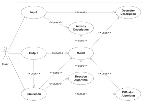
4.1.3 Use-Case Descriptions . . . 39
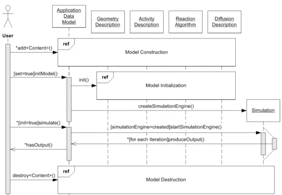
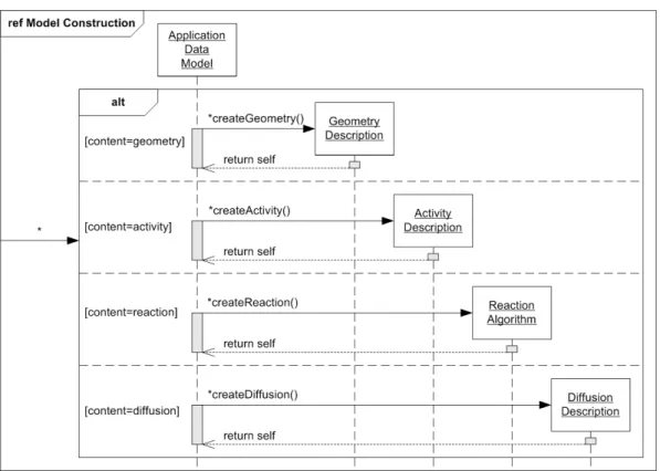
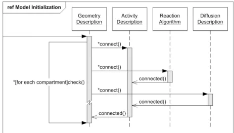
4.1.4 Program Dynamics . . . 41
4.2 Considerations and Definitions . . . 45
4.2.1 Geometry Model . . . 46 4.2.2 Activity Description . . . 55 4.2.3 Algorithm Handling . . . 65 4.2.4 User Interfaces . . . 73 4.3 Application Details . . . 74 4.3.1 User Interfaces . . . 78 4.3.2 Applicability . . . 80 4.3.3 Complexity Considerations . . . 81 4.3.4 Availability . . . 82
5 Applications, Results, and Analysis 83
5.1 Application Development . . . 84
5.1.1 Plug-Ins . . . 84
5.1.2 Programming Languages . . . 86
5.2 Modeling and Simulation . . . 86
5.2.1 Simple Diffusion Simulation . . . 87
5.2.2 Applying Diffusion-Reaction Systems . . . 89
5.3 Comparing Tools . . . 93
5.3.1 Comparison Criteria . . . 94
5.3.2 Comparing Related Works . . . 94
5.3.3 In Comparison to 4DiCeS . . . 100
5.4 Related Work . . . 101
6 Conclusions 103 6.1 Design Decisions . . . 104
6.2 Related Attempts . . . 105
6.3 Challenges and Accomplishment . . . 108
6.3.1 Model Complexity . . . 108
6.3.2 Performance Evaluation . . . 110
6.4 Outlook . . . 110
A Algorithms in Detail 113 A.1 Reaction Algorithms . . . 113
A.2 Diffusion Algorithm . . . 118
B Backus–Naur Form 121 C Unified Modeling Language 123 C.1 Use-Case Diagrams . . . 123 C.2 Class Diagrams . . . 125 C.3 Sequence Diagrams . . . 126 C.4 Component Diagrams . . . 127 List of Abbreviations 129 List of Figures 133 List of Tables 135 Bibliography 137
CHAPTER
1
Introduction
1.1
Motivation
The emerging field of systems biology allows for the application and combi-nation of experimental, theoretical, and modeling techniques. A key goal of systems biology is to understand biological processes as whole systems instead of isolated parts. With such a systems-level analysis, the study of biological phenomena at the molecular, cellular, or behavioral levels becomes more feasi-ble (Kitano, 2002b; Kell, 2004). Improvements in the measurement of molecular interactions and rates have revolutionized our insight into the cell and its dy-namics. An enormous amount of information has been gained over the past decades adding to the already-known mechanisms. This leads to a vast set of parameters making it difficult to evaluate new hypotheses on intuition alone. Thus, applying modeling techniques and computer simulations help to confirm such hypotheses (Kitano, 2002a; Shapiro et al., 2002).
In recent years much progress in the development of cell-biological modeling and simulation tools has been achieved. A multitude of existing programs can already fulfill the major requirements of execution speed and result accuracy. However, often such programs are highly specialized in their methodology and the applications they were designed for. There is no system that allows for the use of more than one algorithm in a simulation at a time. Furthermore, the existing tools are still behind on the development of three-dimensional (3D) visu-alization techniques. In comparison to existing two-dimensional (2D) simulation applications, the 3D approaches are still at their early stages. The additional spatial information allows for a more direct referencing of the model to its real object. Methods applied to 3D share many characteristics with 2D techniques. Many existing 2Dmethods therefore can be either adopted or carried forward. Along with mechanistic models it is often possible for system behavior to be for-malized into solvable differential equations. On the basis of such equations the evolution of time is regarded as predictable as well as continuous and is there-fore a very fast and precise method (Ghosh and Tomlin, 2004). Nevertheless,
deterministic approaches to model and simulate the dynamics of intracellular regulatory processes have their limitations. For the reason of combinatoric in-crease in the number of equations and the number of contained players this process becomes highly impractical. If only small numbers of particles are in-volved, deterministic modeling approaches and simulation might fail. Stochas-tic approaches, using closer knowledge of the subcellular architecture, are more appropriate in these situations (Kiehl et al., 2004).
A significant obstacle with given modeling and simulation tools is that they seem to be able to handle only a small set of applications. They were developed for simulating special models and lack the ability to integrate extra techniques for solving other problems. In fact, often systems focus their attention on handling a special problem to all its details in minimal computational time (Pettinen et al., 2005). The currently used programs therefore vary noticeably in their applicability for specific types of modeling. Moreover the integration of such programs is highly demanding. They are closed systems and often do not offer component interfaces. In practice it could be beneficial to allow for such interfaces to combine various different tools to just one tool only. A compromise to the absence of direct interfaces is the possibility of exchanging information via standardized file formats. For this, many tools use the Systems Biology Markup Language (SBML) as a standard (Hucka et al., 2004). Often, by the use of such standardized formats, important information to the model cannot be handled correctly and might get lost. Especially withSBML, the geometrical information cannot be saved entirely and subsequently has to be reconstructed. Applications for such a modeling and simulation tool that allows for both 3D visualization and concurrent algorithms are imperative. The applications lie in the areas of electrical excitable cells, circadian rhythm, cell cycle, cellular motility, membrane transporters, metabolic pathways, and signal transduction networks. In comparison to 2D methods, the use of a 3D geometry provides considerably more significant data. The possibility of simulating different com-partments of a cell with diverse algorithms can reduce computational effort dramatically. Consequently, this allows for both improved modeling and more information output on the spatio-temporal behavior of a system. Thus it is a scientific challenge to integrate concurrently running algorithms in combination with 3D visualization.
1.2
Objectives
This work addresses the problem of an in silico biology system-level analysis on the base of cellular signaling networks. Grounded on biological observations, computational simulation models for the calcium(II) (Ca2+) signaling pathway were developed in an attempt to understand the non-linear dynamics of the system.
To create this kind of an all-encompassing application, several existing sim-ulation systems were evaluated for their strengths and weaknesses. Current state-of-the-art cell simulation applications are either limited to a 2D represen-tation of a cell or do not use any cellular geometry at all. The only exceptions to this finding are the deterministic simulator “VirtualCell”, the stochastic simulators “MCell” and “SmartCell”, as well as this approach of a hybrid four-dimensional (4D) Cell Simulator (4DiCeS). Despite the great variety of software packages available for modeling, simulation, and analysis of data (Hucka et al., 2004) as described above, there was no application that features the complete and variable integration of different simulation methods in a 3D environment. The key improvement, which4DiCeS has over the other existing systems, is the ability not to be fixed on either deterministic or stochastic modeling and sim-ulation approaches. A system of specialized interfaces therefore was designed to allow the bonding of interchangeable algorithmic modules of various types. The internal representation of the model is designed for the easy exchangeabil-ity of data. Furthermore, the integration of cell model file format standards is permitted by exchangeable plug-ins. The implemented system includes an Ap-plication Programming Interface (API) for writing individual plug-ins to utilize different simulation algorithms. This facilitates the implementation of tailored programs and specific algorithms that can be developed for data mining as well as visualization. The resulting 4DiCeS framework presented in this work describes a concept for the integration of heterogenous data into an easy-to-use software.
1.3
Structure
This thesis is primarily concerned with the simulation of cellular phenomena. An application is provided to utilize hybrid mathematical models and to sim-ulate 4D spatial dynamics within a cell. The work reveals that a 3D cellular geometry holds extended information of importance, and is closest to reality in its model and simulation. Also, an application framework will be shown that allows for the integration of various particle reaction and diffusion algo-rithms. Such algorithms can then be applied to a model either in sole or even in concurrency.
The work is divided into three parts. The first part (Chapters 1, 2, and 3) provides this motivation and an introduction to the topic of cellular dynamics, and its modeling and simulation. Relevant current modeling and simulation application will be introduced. The second part consists of Chapter 4 and focuses on the formal description, design, and the methodology of the 4D cell simulator. The third part (Chapters 5 and 6) presents a comparison of related works with the results of the project, discusses this work, and gives a brief outlook on further improvements to the system.
A condensed summary of all chapters of this work is provided with the following overview:
Chapter 2 reviews biological concepts of systems biology as well as mathe-matical aspects of modeling, simulation, and analysis of cellular dynamics.
Chapter 3 describes a number of existing systems that represent state-of-the-art biochemical modeling and simulation applications.
Chapter 4 focuses on the formal description as a basis for the design of the 4DiCeS framework for systems biology.
Chapter 5 comprises the results that were obtained during development and testing 4DiCeS.
Chapter 6 evaluates and discusses the 4DiCeS platform including some ideas that will illustrate further development and directions.
CHAPTER
2
Dynamics in Systems Biology
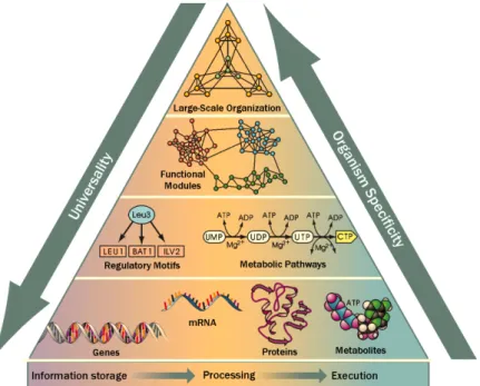
During the past century much progress was achieved in the measurement of cellular processes, molecular interactions, as well as their kinetics. Thus, a revolution was initiated in the understanding of the dynamics within biological cells. The following Figure 2.1 of a pyramid composed of different molecules wants to give insight into the complexity of cellular organization.
Figure 2.1: Life’s complexity pyramid. The genomic information is both stored and translated into functional units such as proteins and metabo-lites. These units form operational molecules, consisting of regula-tory systems or metabolic pathways. On top of these rather small units, large scale organizations implement the characteristic features of an organism. Adapted from Oltvai and Barab´asi (2002).
The fundamental units are arranged to either metabolic and signaling pathways or to motifs in genetic-regulatory networks. Motifs and pathways are linked to operational groups that are responsible for discrete cellular functions (Hartwell et al., 1999). Such groups are then nested hierarchically and characterize the
large-scale organization of a cell (Ravasz et al., 2002).
While creating models of cellular dynamics, one has to understand complex properties. Such properties include the combination of regulatory mechanisms and interlocking transport in and among cells. Electrical activity, signal trans-duction, or other biochemical networks are examples of intricate behaviors tak-ing place on the cellular level. In general such dynamic phenomena refer to arbitrary processes occurring and therefore changing over time. This forms the highly dynamic basis for living cells. To maintain the typical characteristics of a cell’s life such as growth, movement, responsiveness, cell division, and inter-cellular communication, cells must continuously obtain energy from their direct neighborhood. Therefore cells need to act far from static thermal equilibrium as thermodynamically open systems. Hence, cells require a huge amount of energy to sustain the gradients of metabolites and ions in order to function properly (Fall and Keizer, 2002).
The following two Sections 2.1 and 2.2 give an overview on the scope of modeling and simulation of such dynamic systems within cells. By doing so, the need for simulation tools, such as the 4DiCeSsoftware presented here, handling such models becomes apparent.
2.1
Modeling and Simulation
Theoretical methods joined with experimental measuring have offered compre-hensive perception of dynamics for many years (Ortoleva et al., 2003). Comput-ers have demonstrated to be a necessity in assisting the dissection of molecular processes. Yet, the bare amount of quantitative experimental cellular informa-tion allows for the cooperainforma-tion of computer science and biology (Chong and Ray, 2002). The interaction of theory, experiment, and computation succeeds a conceptual formulation analog to successfully proven physical models (see Table 2.1).
Here all modeling is an abstraction of reality. The only exact model of any system is the system itself. So when a model of a system is designed, a choice must be made regarding the level of detail and feature types to be included into that model. To a large extent, this is prescribed by the characteristics of the examined system, the type of experimental data available, and the type of questions that are addressed to modeling (Bolouri and Davidson, 2002).
Step Task Description I Experimental
Work
Figuring out the most plausible out of all possible molecular mechanisms as an initial step.
II Schematic Description
Define a schematic description that characterizes the entire model from such selected mechanisms.
III Mathematical Expressions
Translate the elementary steps of the mechanism into mathematical expressions.
IV Differential Equations
Combine the changes in time described by such ex-pressions into differential equations.
V Analysis Reveal the model’s success for the biological system from the differential equations’ study.
Table 2.1: Conceptual formulation of models. Here, the interdependency of experiment, theory, and computation describe the production of a conceptual formulation of models. All given steps depend highly on a close collaboration with experimentalists working at the same problem. Adapted from Fall and Keizer (2002).
The problems theorists encounter in biology are therefore very alike to that in physical sciences. At this level equations are analyzed, if possible simpli-fied, solved, and, most importantly predictions can be made. These predictions are checked by further experiments. Moreover, such experiments may disclose discrepancies that in turn will require changes to the model (Alvarez-Vasquez et al., 2005). The procedure addressed here is an improving cycle of approxima-tions where the theoretical model acts as a quantitative hypothesis (see Figure 2.2).
The history of simulation and in silico analysis of biological systems dates back to the earliest mechanical and analogue computers in 1940 (Chance, 2004). The recent progress in quantitative simulation and modeling are due to advances in modern information technology and was enhanced by the recent burst of molecular data. It becomes obvious that future progress in the understanding of biological functions will rely on the development and the use of computational methods (Arkin, 2001). Therefore, the following two Sections 2.1.1 and 2.1.2 give a closer look at both, the roles of biology as well as computation to the modeling of biological cellular systems.
Figure 2.2: Systems biology triad. At the center are the complex biological phenomena. Interpretation of observations and data is supported by computational algorithms. The translation of interpretation to understanding is supported by systems science. In turn, systems science provides a framework for understanding. It indicates hy-potheses to be tested and modified in an iterative cycle of experi-mentation. Adapted from Mesarovic et al. (2004).
2.1.1 Biology as a Model Featurer
Cells show very complex and different behaviors. Single cells are able to con-tract, excrete, move, reproduce, send signals, or even respond to them. Fur-thermore, cells accomplish the energy handling required for such activities. In cooperation cells manage all of the various processes required to perpetuate life as is (Hofmeyr, 1986). However, everything that cells do can be represented in the form of basic natural laws. Although the rules of behavior are rather basic, cells comprise huge and complex networks of interacting substrates. An enormous amount of work was used disentangling only very few of such reac-tion schemes, and it is quite obvious that there are many more such interacreac-tion networks yet to be revealed (Keener and Sneyd, 2001). Table 2.2 gives a brief overview of dynamic behaviors happening on a cellular level. Accordingly, the need for powerful modeling and simulation tools, as 4DiCeS, arises very quickly from the study of such phenomena.
In the subsequent sections the dynamical behavior of Ca2+ signaling for its spatio-temporal patterns (see Figure 2.3) will be discussed in more detail. The modeling and simulation of such a phenomenon were used as examples for testing the 4DiCeS software. The role of computational techniques handling such models is going to be presented in the following subsection.
Phenomenon Description Circadian
Rhythm
Regular changes in cellular processes and behavior that have a period of about one day.
Cell Cycle The event of cell division where one cell proliferates into two descendants with full genome.
Cellular Motility
All cellular movement including the remodeling of cell membranes, cellular travel, and contraction.
Membrane Transporters
Transport catalysts at the membrane acting either as car-riers, pumps, or channels for particles.
Electrical Excitable Cells
The display, acceptance, or propagation of electrical poten-tials along or within cells.
Excitable Oscillation
Coupled mechanism of membrane transporters and electri-cal activity resulting in oscillations.
Non-Excitable Oscillation
Self-contained spatio-temporal oscillations of particle con-centrations within a cell.
Table 2.2: Phenomena of cellular dynamics are here depicted, which have trig-ger events in common. There exist theoretical models and simula-tions for each incident. Extracted from Fall et al. (2002).
(a) 0.5min (b) 1min
Figure 2.3: A spiral wave of Ca2+ ions detected from a dye with microinjection of IP3 into an Xenopus laevis oocyte after 30 and 60 seconds. By courtesy of James D. Lechleiter, University of Texas, USA.
2.1.2 Computation as a Model Solver
Techniques applied to research problems in systems biology comprise very much of applied mathematics and computer science. A majority of features in compu-tational modeling of cell biology play an important role. One of these features is the development of algorithms and techniques that give tools for numerical analysis (Takahashi et al., 2002). The computation of mathematical problems on computers is basically an estimation process. The efficiency and accuracy of these methods of estimation are the subjects of intensive study. The work on constructing models is also basically an approximation process. This is due to necessary simplifications that must be used to produce a helpful model. These simplifications must both be valid in terms of the physical process being studied and from a mathematical point of view (Eungdamrong and Iyengar, 2004). Computer models allow for testing conditions that may be difficult to obtain or that have not been examined in the laboratory yet. Therefore, every solution of a mathematical model may offer a simulation of a potential or real experiment. Such simulations can help to estimate parameters, i.e. diffusion or kinetic constants, that are challenging to collect in experiments. Simulations can verify how pharmacological agents may affect a biological process (Mendes and Kell, 1998). Hypothesis about the role of individual mechanistic components can be checked by simulations. Accordingly, predictions made by such simulations then can be tested in the laboratory. It has to be noted that often the most important result of a simulation is a negative one. Therefore, a well-crafted model has to be redefined and tested again (Fall and Keizer, 2002).
Improvements in numerical analysis as well as computer hardware have made the solving of complex deterministic systems accurate and fast. However, mod-els of biological processes almost always comprise nonlinear components in their control mechanisms. By using traditional mathematical methods, as coupled Ordinary Differential Equations (ODEs), often such problems can be solved exactly. But nonlinearities often create difficulties in getting any exact solu-tion. Admittedly, good estimates of nonlinearities can be obtained by using computer implemented numerical methods. Often a major property in cellular mechanisms is spatial variation. Therefore, the analyzing and the solving of spatially explicit Partial Differential Equations (PDEs) is very important. Such PDEs can be more complex and less analytically tractable than ODEs.
Some models need to handle noise and the tracking of single particles instead of particle concentrations. Here stochastic methods such as Monte Carlo (MC) simulations (Metropolis and Ulam, 1949) come into play. Such discrete models
facilitate the qualitative modeling and are based on various different computa-tional approaches (Hofest¨adt and Meineke, 1995). Unlike the different deter-ministic methods, a stochastic approach does not approximate the model as a continuous macroscopic system. In contrast, it treats a model as a discrete and microscopic process. However, this increase in accuracy comes at high costs as each individual chemical entity has to be modeled as a stochastic process. Hence, stochastic simulations are computationally more demanding (Pucha lka and Kierzek, 2004).
Method Description
ODE A relation that contains functions of one independent variable involving its derivatives.
DAE Coupled ODEs with additional algebraic constrains (no deriva-tives).
PDE Differential equations with more than one independent variable involving partial derivatives.
SDE Differential equations including a random term that describes intrinsic noise.
MC A set of discrete quantities and associated probabilities for in-teractions.
Boolean Network
A conversion of a model into a binary representation of only “true” and “false” states.
CA Collection of different elements (cells) with distinct states on a grid of specified shape.
Bayesian Network
Acyclic directed probabilistic graph with random variables (nodes) and conditional independence assumptions (arcs). Petri Net Modeling for concurrent systems with a bi-partial directed
graph. Generalization of the automata theory.
Table 2.3: Important modeling and simulation techniques. The given methods represent the main approaches by which modeling and simulation are handled in systems biology. Applications vary in their support for either a pure method’s implementation or hybrid attempts mixing different techniques. Extracted from Hucka et al. (2004).
Various attempts have been made to construct and simulate biochemical be-haviors. The majority of approaches depend on the use of the before men-tioned deterministic and stochastic techniques (Hucka et al., 2004). Recently other well-established techniques have been applied including boolean networks (Kauffman, 1969), Cellular Automata (CA) (von Neumann, 1966), Bayesian networks (Pearl, 1988), and petri nets (Petri, 1962), to biological applications. Hybrid methods that combine the best features of all approaches exist as well (Lu et al., 2004). Table 2.3 summarizes some highly recognized basic techniques for modeling and simulation in systems biology.
To solve equations that result from a model is only one part of the work. The other side needs to comprehend the model’s behavior. Mathematical methods were developed for the system analysis of models that characterize complex pro-cesses. Such methods disclose the dynamical behavior, properties, and struc-ture of the system. This is very much as molecular biological, physiological, and anatomical techniques uncover the physical basis of the model (Hartwell et al., 1999). Hence, the analysis exposing complicated behaviors within a model may result in further study of these biological phenomena. Admittedly, decisive analysis of complex equations demands skill. This is due to the fact that there are many intricacies that can only be comprehended through intensive train-ing (Mishra et al., 2003). The construction and alteration of simple models is within the reach of cell biologists. Therefore it is necessary for scientists to seek association with mathematicians and computer scientists for the effectual simplification of complex models (Sontag, 2004).
The next section will go into the detail of a well-studied Ca2+ model systems. This model was chosen to test the 4DiCeS software in its functionality and accuracy. The next chapter on the other hand will give insight into the design of the4DiCeSsystem itself. After reading these sections, it will become obvious that the application should be capable of applying any of the before mentioned mathematical techniques. As for now stochastic and deterministic methods are implemented to be used by 4DiCeS (Oleson et al., 2006).
2.2
Cellular Calcium Models
Cellular Ca2+ has an overall very low concentration. At rest it is approximately 0.1µM, and only about 1–10µM at its peak. On the other hand, potassium (K+) and sodium (Na+) show millimolar concentrations. Cells require to keep
cyto-plasmic Ca2+ concentration ([Ca2+]
i) at low levels due to the fact that Ca2+ can modify the enzymatic properties of binding proteins. Hence increases in the cellular Ca2+ level are locally defined and quick to circumvent the runaway activation of enzymatic cascades. Two basic mechanisms hold responsibility for this impoundment and buffering. The buffers are highly specialized Ca2+ -binding proteins that absorb 95–99% of the cytosol’s Ca2+. Ca2+ is impounded to either the sarcoplasmic reticulum (SR) in muscle cells or the endoplasmic reticulum (ER) in all other cell types. Proteins hydrolyze adenosine–3’,5’– triphosphate (ATP) to transportCa2+ against rampant concentration gradients. Such proteins are ATP hydrolases (ATPases) that are classified as SR/ER Ca2+ -transport ATPase (SERCA) pumps. On the other side, plasma membrane (PM) Ca2+-ATPase (PMCA) pumps dispose Ca2+ of the cell. SR and ER membranes have ion channels, which are different from PMCAs, that transports Ca2+ back into the cytoplasm. Therefore, every cell has Ca2+ pumps for homeostasis as well as negative feedback. Some cells have developed ion channels such as the inositol–1,4,5–trisphosphate (IP3) receptor (IP3R), which is activated and in-hibited by Ca2+. The IP
3R is able to give both positive and negative feedback. Thus, brief channel openings may enable oscillations of free cytoplasmic Ca2+ that are utilized for signaling. Interestingly, Ca2+ oscillations were discovered in vitro after they were predicted by a model (Chay and Keizer, 1983).
2.2.1 Calcium Signaling
Ca2+is the most common cellular signals’ carrier. Due to its special adaptability as a ligand, it regulates very many important aspects of cellular activity. This goes from the creation of new life at fertilization to the radical incident of cellular apoptotic suicide. Signaling byCa2+ shows a number of properties that make it unique among all other carriers of signals. An important example is its ability to function both as a first and as a second messenger (Carafoli, 2005). ThenCa2+cannot be metabolized like other second-messenger molecules. Hence cells tightly regulate intracellular levels through numerous bindings as well as specialized extrusion proteins (Clapham, 1995).
Almost all eucaryotic cell types use both intracellular as well as extracellu-lar resources of Ca2+. The responsible regulating mechanisms for the influx of externalCa2+ are already well known to scientists (Carafoli, 2002). As an exam-ple, voltage-operated channels in neurons assist action potentials by triggering the release of neurotransmitters at synaptic junctions. Neurotransmitters can establish an influx of Ca2+ utilizing receptor-operated channels primarily
local-ized postsynaptically. Despite such well-established influx pathways, there is not much known on the mechanism of the intracellular Ca2+ supply of neurons although IP3Rs allocated all over the ER are accountable for the dispense of Ca2+ (Berridge, 2005).
TheERnetwork in cells accounts for the dynamics ofCa2+signaling by operating both as a sink as well as a source of Ca2+. Such an internal storage of Ca2+ is possible to have a far reaching impact on Ca2+ signals in cells. Ca2+ can be localized within compartments in high levels or can spread across cells as widespread Ca2+ waves (Berridge, 1998).
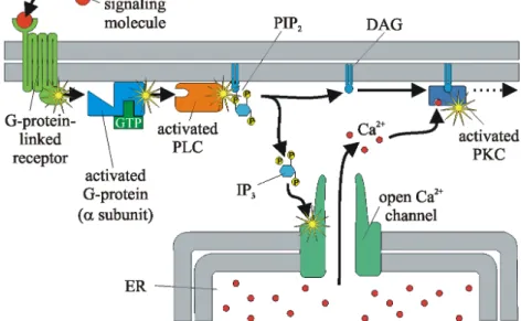
TheIP3signaling network (see Figure 2.4) is highly sophisticated within cell tis-sues. A manifold amount of diverse receptors excite the hydrolysis of phosphat-idylinositol-4,5-bisphosphate (PIP2) into IP3 and sn–1,2–diacylglycerol (DAG). Both are well known second messengers. IP3 then releases Ca2+ from the ER’s IP3Rs (Berridge, 1993).
Figure 2.4: The Ca2+ signaling pathway. When a hormone or neurotransmitter (“first messenger”) interacts with a receptor on the cell membrane, IP3 is released within the cell, causing a calcium response. The ER plays a decisive role in calcium regulation next to the extracellular space as a storage for the cytotoxic Ca2+. Adapted from Alberts et al. (2003).
By the fact that the intracellularCa2+ release byIP
3Rs is sensitive to a diversity of different factors makes it very complex. IP3Rs are most effectively activated
when Ca2+ and IP
3 are both presented at the same time. This dual activation has noteworthy effects for signal transduction mechanisms. Foremost of these is that theIP3receptor may act as a cooccurrence detector due to the requirement for two separate messengers. Small levels of IP3, unable to excite an immedi-ate Ca2+ release, may enhance the IP
3R’s Ca2+ responsiveness. Thereby they change the cytoplasm into a medium capable of producing regenerative Ca2+ waves. An increasing Ca2+ gradient within the ERcan have a positive feedback by sensitizing the IP3Rs’ Ca2+ uptake. The increase of [Ca2+]i represses IP3Rs (Berridge, 2004).
2.2.2 Two Pool Model
The two pool model presented in this section is based on the works of Goldbeter et al. (1990); Berridge (1991). This model shows an oscillating behavior of Ca2+ concentrations very similar to phenomena discovered in living cells. If a diffusion term is applied to the system even 3D wave-fronts can be simulated. The basis of the two pool model is that oscillations are set up through an interaction between two releasable pools of Ca2+. Here it is assumed that the external signal triggers the synthesis of IP3. The effect is simply a discharge of an intracellular pool of Ca2+ leading to a rise of cytosolic Ca2+. A simple assumption is made that a constant influx of Ca2+ from the IP3-sensitive pool occurs as long as the stimulus is present. This affects the probability of the occurrence of oscillations exclusively by the cycling of Ca2+ between the cytosol and the IP3-insensitive pool. The IP3-insensitive pool is therefore considered to remain constant as a result of a fast backfill by the influx of extracellular Ca2+ (Goldbeter et al., 1990). This autoregulatory mechanism is controlled by the content of Ca2+ in the IP3-sensitive pool and by the uptake of cytosolic Ca2+ after a spike. The magnitude of the influx, v
1β, from this IP3-sensitive
pool is assumed to be proportional to the saturation function β of the IP3R. The cooperative nature of this saturation function is expressed implicitly in
β. The level of IP3 is proposed to be caused by stimulation increases with the magnitude of the external signal. IP3 thus controls the flow of Ca2+ into the cytosol. This again assists the IP3-insensitive pool for releasing Ca2+ in oscillatory cycles (Berridge, 1991).
The two variables of this model are the concentration of free Ca2+ in the IP 3-insensitive pool (e.g., the ER or SR) and in the cytosol. These two variables are denoted by Z and Y, respectively. If assumed that buffering is linear with
respect to the Ca2+ concentration, then the time evolution of the system is driven by the following two kinetic equations (Goldbeter et al., 1990):
dZ
dt = v0 +v1β−v2+v3+kfY −kZ, (2.1) dY
dt = v2 −v3−kfY . (2.2)
In the above equations, all rates and concentrations are defined with respect to the total cell volume. Here, v0 and kZ relate to the influx and efflux of
Ca2+ into and out of the cell. This occurs even in absence of external stimuli. These terms are assumed to be constant and linear for simplicity. The rate of ATP-driven pumping of Ca2+ from the cytosol into the IP3-insensitive store is denoted with v2. In contrast v3 represents the rate of transport from this pool
into the cytosol. The term kfY refers to a leaky, non-activated transport from
Y intoZ. This process was found to stabilize the amplitude of Ca2+ transients at different levels of stimulation.
An increase in IP3 is triggered the reception of an external signal. This in turn leads to a rise in the saturation function β and to a subsequent increase of cytosolic Ca2+. The conditions in which this initial rise triggers Ca2+ oscilla-tion can be determined by resorting to phase plane analysis. This is especially possible because the system of equations comprises only two variables. Here, it was indicated that the activation of v3 by Z is most appropriate for inducing
sustained oscillations upon external stimulation. This condition directly corre-sponds to an activation by cytosolic Ca2+ where Ca2+ is transported from the intracellular store into the cytosol. The two pool model predicts that at least in the absence of time delays, such a process does not satisfy the triggering of a sustained oscillatory response. When taking into account the cooperative nature of the pumping process, the Ca2+ release from the intracellular store, and the positive feedback performed by the latter transportation of cytosolic Ca2+, the rates v2 and v3 in the equations 2.1 and 2.2 take the following form
(Goldbeter et al., 1990): v2 =VM2 Zn Kn 2 +Zn , (2.3) v3 =VM3 Ym Km R +Ym × Z p KAp +Zp . (2.4)
In these equations, VM2 and VM3 denote respectively the maximum rates of
Ca2+ pumping into and the release from the intracellular store. These processes are described by Hill functions whose cooperativity coefficients are taken as n
and m. Here, p denotes the degree of cooperativity of the activation process.
K2, KR, as well as KA are threshold constants for activation, pumping, and
releasing.
The equations 2.1, 2.2, 2.3, and 2.4 admit a unique steady-state solution. Linear stability analysis of these equations indicated that the steady state is not always stable. In the absence of stimulation, a situation is considered in which the system is initially in a stable steady state characterized by a low cytosolic Ca2+ level close to 0.1µM. The system reacts to an increase in β up to 30%, due to a rise in IP3 triggered externally. Here, an oscillation of cytosolic Ca2+ occurs. Such repeating spikes are accompanied by a sawtooth variation of the intracellular store’s Ca2+ content. The period of the oscillations is of the order of 1s, as in some experimental systems. Periods of 1min or more are readily obtained if the kinetic parameters are divided by a factor of 10–100 (Kraus and Wolf, 1992). A spatio-temporal extension of the two pool model allows for the modeling of intercellular Ca2+-waves. To make this happen a diffusion term has to be added to the system. In the model it is assumed that the IP3-sensitive Ca2+ pools are only located near the membrane and the IP3-insensitive pools are spread all over the intracellular space.
The mathematical description of the deterministic methods account the system with a coupled set of nonlinear ODEs of first order. Kraus et al. (1992); Kraus and Wolf (1992) derived a stochastic model from this system, which is numer-ically traceable by means of a stochastic simulation. The stochastic method models the system through a master equation. With the first method the pools correspond to particle concentrations and the processes correlate with mathe-matical functions, which move into the pools via fluxes connected with concen-trations. With differentiation of the master equation the pools contain a certain number of particles. Now the process describe transition probabilities between state transitions, which are connected by fluxes. The states are characterized by the overall occupation number of the pools. External entities comply in both cases with externally defined system parameters. While the deterministic method inspects the temporal trend of concentrations, the stochastic method describes changes in particle numbers of every particle species in contrast to that. Each reaction, where the number of particles changes, is simulated di-rectly. The stochastic method therefore constitutes the microscopic view of the system, which is in diametric opposition to the deterministic - and thus
macroscopic - depiction.
The stochastic model was applied to the simulator described in this work for final a testing and comparison purpose of state-of-the-art modeling and simu-lation tools in Section 5.2.2.3. The mathematical formusimu-lation of the stochastic two pool model is displayed in Table 2.4.
Reaction Transition Probability State Transition Ca2+ex k1 −→X k1Ca2+ex ≡v0 X →X+ 1 Y = const X −→k Ca2+ex kX X →X−1 Y = const Ca2+ISCS −→k2β X k2Ca2+ISCSβ ≡v1β X →X+ 1 Y = const Y −→kf X kfY X →X+ 1 Y →Y −1 pX +mY v 0 3 −→(m+p)X v3 =VM3 Y m Km R+Ym × Zp KAp+Zp X →X+m Y →Y −m nX v 0 2 −→nY v2 =VM2 Z n Kn 2+Zn X →X−n Y →Y +n
Table 2.4: Stochastic two pool model. This table specifies the mathematical process of the stochastic two pool model. X and Y describe the number ofCa2+ ions in the cytosol or theIP3-insensitive pool. There is the assumption that the number of Ca2+ ions in the extracellular space and within theIP3-sensitive pools are kept constant. Adapted from Kraus et al. (1992).
Chapter 3 now gives a closer look on currently used simulation software tools. Their architecture and utilized algorithms will be continued and compared in Chapter 5 with a preceding formal description on 4DiCeS (see Chapter 4).
CHAPTER
3
Related Approaches and Tools
The relevance to model as well as to simulate biological systems was discussed in the previous chapter. The following chapters give an overview of the state-of-the-art in modeling and simulation in comparison to the new cell biology framework 4DiCeS. Therefore, some of the inherent problems in characteriz-ing the different facets of biological function are stated. This includes a brief overview of how functional information is currently represented in databases. And also prevailing applications for modeling and simulation of biochemical networks are introduced.
3.1
Database and Information Retrieval
The tremendous but valuable information gathered together in recent years has to be organized and pooled in databases. In this respect databases are widely deployed to store the relationships of biochemical systems. Currently there exist over 1000 biological databases (Galperin, 2008) and about 45 databases supplying cellular signaling pathways at different levels of detail and complexity. Public bio-molecular interaction databases are resources to basic building blocks of biological signaling pathways. Huge clusters of molecular interactions can be generated based only on this information. However, a molecular interaction cluster does not represent a signaling pathway per se. In effect, more infor-mation about each interaction, such as its outcome (e.g. activation as well as inhibition), is required for it to become a trustful component of a signaling pathway (Cary et al., 2005). Both public as well as private database initiatives have taken up the effort of creating biological pathway databases and pro-viding computational biology tools for their analysis. Some of the databases focus on static (manually drawn) representations (Bhalla and Iyengar, 1999; Sivakumaran et al., 2003; Trost, 2002) whereas other systems support dynamic visualizations based on graph drawing algorithms (Fukuda and Takagi, 2001; Fukuda et al., 2004)). There is also a variety of databases specialized in molec-ular pathways with physical parameters as rate constants and concentrations (Igarashi and Kaminuma, 1997). In addition to the previously described
path-way databases, there exist databases containing detailed information regarding characterized enzymatic reactions. Additional links to other databases provide useful information on involved enzymes and biochemical reactions (Gough and Ray, 2002; Gough, 2002).
Currently three simulation model repositories serve actively in the internet – namely the Cell Markup Language (CellML) (Lloyd et al., 2004), the JWS Online (Olivier and Snoep, 2004), and the BioModels (Nov`ere et al., 2006) repository (see Table 3.1).
Designation Web Site
BioModels http://www.ebi.ac.uk/biomodels/ Cellerator http://www.cellerator.info/nb.html CellML Repository http://www.cellml.org/models/ JWS Online http://jjj.biochem.sun.ac.za/
xCellerator http://www.xcellerator.info/examples/index.html
Table 3.1: Model repositories. The simulation model repositories of the two most prominent modeling languagesSBML and CellMLcontain mod-els on metabolic networks, cell cycle and cellular signaling. The (x)Cellerator sites provide example models as Mathematica (*.nb) files. The SBML (Hucka et al., 2004) repository ceased work at the end of 2005. The E-Cell project (Takahashi et al., 2003) has plans for its own model repository, however, there is no concrete data available on the internet at present.
Further information on biological pathway databases can be retrieved from the Nucleic Acids Research database issues (Baxevanis, 2000, 2001, 2002, 2003; Galperin, 2004, 2005, 2006, 2007, 2008) and by the Pathway Resource List (PRL)1 – a database that contains information on over 240 internet
path-way resources. Most of these resources are databases themselves containing protein–protein interactions, metabolic reactions, or cellular signaling. The PRL provides resource links and is building up additional information such as the amount of data and the organism coverage within each pathway resource (Bader et al., 2006).
3.2
Modeling and Simulation Software
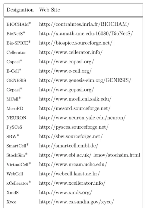
The preceding section gave a brief introduction to an overwhelming amount of data repositories present for use in systems biology. The amount of simulation tools dealing with biochemical reaction and diffusion systems is not quite as huge, but is still plentiful. Therefore, this section deals with the description of only the most important applications of this category (see Table 3.2).
A simulation tool is defined as an application performing time series simulation of predefined mathematical models. In contrast a design or modeling tool is applied for building a model graphically. Often simulation tools bring an attached design tool along. If not then models can either be described by markup or scripting languages (Pettinen et al., 2005).
The simulation software tools can be categorized into either deterministic, stochastic, or hybrid (deterministic and stochastic) programs. Other cate-gories apart from the algorithmic approaches are the modeling of either 2D or3D geometry and the separation of programs into either stand-alone tools or frameworks.
One of the very first programs available for reaction simulations was the GEn-eral PAthway SImulator (Gepasi) (Mendes, 1993). It translates biochemical reaction equations into coupled ODEs which in turn are then solved numeri-cally. Thus the Gepasi system represents a purely deterministic approach such as BIOCHemical Abstract Machine (BIOCHAM) (Calzone et al., 2006), Celler-ator (Shapiro et al., 2003), E-Cell, the Python Simulator for Cellular Systems (PySCeS), and VirtualCell do as well (see Section 3.2.1). The deterministic sim-ulators Genesis and Neuron were originally designed to model neurons and neuronal networks but have shown that cell signaling simulations are just as adequate (Bhalla, 2002). Xyce is actually a deterministic massively parallel simulator for electronic circuits that was used for solving biochemical problems (Schiek and May, 2003). Simulators such as the Stochastic Simulator (StochSim), the MC Simulator of Cellular Microphysiology (MCell) (see Section 3.2.2), and Mesoscopic Reaction Diffusion (simulator) (MesoRD) (Hattne et al., 2005) im-plement stochastic algorithms only. Examples for hybrid simulators are the Bio-chemical Network (stochastic) Simulator (BioNetS) (Adalsteinsson et al., 2004), the PySCeS (Olivier et al., 2005), WebCell(Lee et al., 2006), and xCellera-tor.
Very recently, efforts have been made to mix various approaches in order to obtain either the combination of many tools in one software package (Rost and
Designation Web Site BIOCHAM* http://contraintes.inria.fr/BIOCHAM/ BioNetS* http://x.amath.unc.edu:16080/BioNetS/ Bio-SPICE* http://biospice.sourceforge.net/ Cellerator http://www.cellerator.info/ Copasi* http://www.copasi.org/ E-Cell* http://www.e-cell.org/ GENESIS http://www.genesis-sim.org/GENESIS/ Gepasi* http://www.gepasi.org/ MCell* http://www.mcell.cnl.salk.edu/ MesoRD http://mesord.sourceforge.net/ NEURON http://www.neuron.yale.edu/neuron/ PySCeS http://pysces.sourceforge.net/ SBW* http://sbw.sourceforge.net/ SmartCell* http://smartcell.embl.de/
StochSim* http://www.ebi.ac.uk/ lenov/stochsim.html VirtualCell* http://www.nrcam.uchc.edu/
WebCell http://webcell.kaist.ac.kr/ xCellerator* http://www.xcellerator.info/ XmdS http://www.xmds.org/
Xyce http://www.cs.sandia.gov/xyce/
Table 3.2: Simulation and modeling environments. This table presents a subset of software tools available today for cellular modeling and simulation. Shown here are 20 out of more than 80 applications. The simulators BioNetS, Copasi, MCell, SmartCell, and StochSim are stochastic applica-tions. The SBW and the Bio-SPICE are actually simulation frame-works rather than programs. The remaining applications within this table are based on deterministic modeling and simulation. A special position take XmdS and BioNetS as they are code generators. The
Kummer, 2004), e.g. the Complex Pathway Simulator (Copasi) (see Section 3.2.2) or a tool offering access to many different software packages, e.g. the Systems Biology Workbench (SBW) (see Section 3.2.3). A very special position takes the eXtensible multi-dimensional Simulator (XmdS) and BioNetS as they actually are C++ code generators (Collecutt and Drummond, 2001). If their code is compiled then the resulting programs are simulation applications by their own again. Further information on existing modeling and simulation applications can be retrieved by the SBML Software Guide2 – a matrix that
contains information on software providing support for SBML.
The following three sections give a closer look to ten well reputed applications and two frameworks. The last Section 3.2.4 then defines comparison criteria for the comparison of the ten programs. The 4DiCeS approach, which will be presented in the subsequent Chapter 4, is going to be brought into context with Section 5.3.
3.2.1 Deterministic
This section presents five well known and used deterministic simulation appli-cations. Although Gepasi ceased further development, it is still in use to date and has played a major role in the development of all the other tools discussed here. There are plans to completely replace Gepasi by the newer Copasi (see Section 3.2.2.2). Excepting Gepasi all other described simulators are still under development and have a user community of their own.
3.2.1.1 BIOCHAM
BIOCHAM is a programming environment for modeling biochemical systems, making simulations, and querying the model in temporal logic. It provides a rule-based language for modeling biochemical systems, a simulation engine, and a query language based on temporal logic, Computational Tree Logic (CTL), or Linear Temporal Logic (LTL). A machine learning system is provided for correcting and completing models either by changing rules with respect to aCTL specification or by estimating parameters of an LTL specification. An interface to the symbolic model checker (NuSMV) is provided also. BIOCHAMwas initiated by the Constraint Programming group of The National Institute for Research in Computer Science and Control (INRIA) at Rocquencourt, France.
3.2.1.2 E-Cell
The E-Cell project is based on international research aiming to model and re-construct biological phenomena in silico and to develop necessary theoretical supports, technologies and software platforms to allow precise whole cell sim-ulation (Tomita et al., 1997). The E-Cell Model Language (EML), a subset of the eXtensible Markup Language (XML), is used for describing the models. The SBMLsupport was also included to enable a wide cross-platform model ex-change (Tomita et al., 1999). TheE-Cellproject is managed by the Institute for Advanced Biosciences, Laboratory for Bioinformatics, Fujisawa and the Mitsui Knowledge Industry, Bioscience Division, in Tokyo, Japan.
3.2.1.3 General Pathway Simulator (Gepasi)
The GEneral PAthway SImulator is one of the first software packages for mod-eling biochemical systems. Gepasi simulates the biochemical reaction kinetics, provides a number of tools to fit models to existing data, optimizes the functions of the models, and performs a metabolic control analysis and a linear stability analysis (Mendes, 1993). The application simplifies the task of model-building by assisting the user in automatically translating given reactions into matrices and differential equations transparently (Mendes, 1997). This is combined with a set of numerical algorithms that ensure fast and accurate results (Mendes and Kell, 1998). It was developed at the Virginia Bioinformatics Institute, USA, as a pure deterministic modeling and simulation environment.
3.2.1.4 VirtualCell
The National Resource for Cell Analysis and Modeling at the University of Con-neticut Health Center, in ConCon-neticut, USA, created a remote user simulation and modeling application. A general purpose differential equation solver is used to translate the initial biological description into a set of differential equations (Loew and Schaff, 2001). The generated results are stored on a remote server and can be reviewed and exported into various formats. The compartments represent 3D volumetric regions, while the membranes represent 2D surfaces separating the compartments (Schaff et al., 1997; Schaff and Loew, 1999). The geometry may be captured by various imaging modalities, such as wide field, confocal, or electron microscopy (Slepchenko et al., 2002).
3.2.1.5 xCellerator
The xCellerator is the successor to the Cellerator package, which was designed as an interface to Wolfram Mathematicafor facilitating biological modeling by auto-mated equation generation. It provides tools for generating, translating, and numerically solving a potentially unlimited number of biochemical interactions (Shapiro et al., 2003). xCelleratorsolves the complete set of equations predicted by the law of mass action. The package also contains a number of transcrip-tional regulation models that are not Michaelis-Menten equations. xCellerator may write its results in SBML. TheCelleratorpackage was formerly developed at the National Aeronautics and Space Administration’s (NASA) Jet Propulsion Laboratory, California, USA, and is now privately continued.
3.2.2 Stochastic
The simulation applications shown in this section are stochastic approaches (Kibby, 1969). They either implement proprietary algorithms of their own (MCellandStochSim) or make use of simulation algorithms from literature (BioNetS, Copasi, andSmartCell). BioNetS and Copasi are also utilizing numerical solvers in combination to their stochastic algorithms.
3.2.2.1 Biochemical Network Stochastic Simulator (BioNetS)
BioNetSwas developed at the University of North Carolina at Chapel Hill, USA. It was designed to simulate biochemical network models in a hybrid, stochastic and deterministic manner. The type of used discrete or continuous random variable for each chemical species in the network can be specified individually. The package was implemented to efficiently scale with any network size to allow the study of large systems. BioNetS is available as a stand alone package but runs also as a Bio–Simulation Program for Intra- and Inter-Cell Evaluation ( Bio-SPICE) (see Section 3.2.3.1) agent. The output of the software is portable C/C++ code that may be compiled and run on any system with the appropriate compiler (Adalsteinsson et al., 2004).
3.2.2.2 Complex Pathway Simulator (Copasi)
The Copasi project is based on Gepasi and a program for the automatic pars-ing and STochastic simulation of ODEs (STODE)3 (van Gend and Kummer,
2001). Copasi incorporates a model generator, user-friendly visualization plat-forms, optimization routines, methods from non-linear dynamics, and different simulation techniques. Copasi is supervised by Pedro Mendes (Bioinformatics Institute, Virginia, USA) along with Ursula Kummer of the European Media Laboratory, Heidelberg, Germany. This application is planned to enable the simulation of complex metabolic processes in cells without having to master complex mathematical or computer skills (Rost and Kummer, 2004).
3.2.2.3 MCSimulator of Cellular Microphysiology (MCell)
MCell is a modeling application for simulations of cellular signaling in complex 3Dsubcellular micro-environments. OptimizedMC algorithms are used to track the stochastic behavior of discrete molecules in space and time. These particles diffuse and interact with other heterogeneously distributed molecules within the 3D geometry (Bartol Jr. et al., 1996). All simulation components are defined by using a specific programming language called Model Description Language (MDL) (DeSchutter and Cannon, 2000). The project was initiated by the Computational Neurobiology Laboratory at the Salk Institute for Biological Studies, in California, and by the Pittsburgh Supercomputing Center’s working group for Biomedical Applications, Pennsylvania, USA.
3.2.2.4 SmartCell
SmartCellis a general tool for modeling and simulation of reaction and diffusion pathways within cells. It supports diffusion and localization by using a meso-scopic stochastic reaction model. The SmartCell package should handle various cell geometries, allows the localization of species, supports desoxyribonucleic acid (DNA) transcription and translation, membrane diffusion and multi-step reactions, as well as cellular growth. Moreover, different temporal and spatial constraints can be applied to the model (Ander et al., 2004). It is expected to provide a suitable model description format (Nasi, 2004). SmartCellis a project of the European Molecular Biology Laboratory, Heidelberg, Germany.
3.2.2.5 Stochastic Simulator (StochSim)
StochSim was written by Carl Firth as part of his PhD work at the University of Cambridge (Morton-Firth, 1998). It was developed as part of a study of bac-terial chemotaxis as a more realistic way to represent the stochastic features of this signaling pathway. It is able to handle large numbers of individual reactions encountered (Morton-Firth and Bray, 1998; Morton-Firth et al., 1999). The ap-plication consists of a platform-independent core simulation engine. The pro-gram encapsulates the algorithm described above as well as a separate graphical user interface. StochSimrepresents individual molecules or molecular complexes as individual software objects (Nov`ere and Shimizu, 2001).
3.2.3 Frameworks
This section introduces frameworks rather than applications in comparison to the two previous sections. Such frameworks are developed to accomplish very particular problems. They provide entire workbenches of interfaces that allow for the integration of many tools and methods to interact with each other.
3.2.3.1 Bio–Simulation Program for Intra- and Inter-Cell Evaluation (Bio-SPICE)
The Bio-SPICE toolkit was developed to model and simulate cellular dynamic networks. Contributed modules are organized in the Bio-SPICE dashboard, which is a graphical user environment (Sauro et al., 2003). It permits data sources, models, simulation engines, and output displays provided by different investigators, and running on different machines, to work together across a dis-tributed, heterogeneous network (Garvey et al., 2003). Among several other features, the environment enables users to create a graphical workflow by con-figuring and connecting available Bio-SPICE components (Kumar and Feidler, 2003a,b). The project was initiated by the Defense Advanced Research Projects Agency Information Processing Technology Office, Virginia, USA.
3.2.3.2 System Biology Workbench (SBW)
The SBW enables different tools to interact with each other. The framework supports tools written in different programming languages, which may run on different platforms and physical machines (Sauro et al., 2003). The aim is to
facilitate collaboration among developers of systems biology software. Develop-ers should find it easier to build anSBWinterface than to recreate functionality. They can then concentrate on developing best-of-breed solutions in the areas where they have special expertise (Hucka et al., 2002). Both SBW and SBML are being developed in collaboration with several groups developing simulation packages as described in the last two sections.
3.2.4 Comparison
While the described simulation tools thus have their benefits, none have so far addressed all the currently emerging research problems. The efforts in the field of cellular simulation can be roughly categorized as stand-alone modeling and simulation tools or extendable frameworks. The first can then be divided again into either more or less strict deterministic or stochastic methods. Even though the stand-alone tools often provide software interfaces, frameworks broaden this ability to include new technologies to the system.
Specific interests of research groups often have great influence on the devel-opment of simulation applications. The usability of a tool is highly affected by user requirements (Schwehm, 2001). Here the chosen operating system and the selection of a Graphical User Interface (GUI) versus a scripting or batch mechanism are key features. Programs currently used vary noticeably in their applicability for specific types of modeling (Pettinen et al., 2005). The gen-eral usability indicated by the user’s learning curve and application-provided model designers have here a great impact. Well featured textual or graphical utilities often aid the modeling process significantly. The number and quality of the utilizable algorithms, supported model-exchange formats, and additional features round up such user requirements dramatically. Next to this, it is of major importance to have a tool with reliable and precise results at optimal performance. An extension mechanism for the integration of new features and functionality is then crucial. The support of spacial modeling information is necessary for close to reality simulations. And last but not least it is important to segregate parts of the model and handle such parts differently.
The following Table 3.3 will therefore define 12 comparison criteria extracted form the preceding paragraphs. These criteria are applied to the previously introduced related applications in a three-state manner. The three states range from unsatisfactory to sufficient. This will allow for an easier qualification of the differences among the tools. Table 3.4 is then going to summarize all
comparison findings from that definition.
Criteria Description
Accuracy Simulation results are reliable and precise.
Concurrency Various algorithms can be handled in concurrency. Designer Modeling is supported by textual or graphical utilities. Exchange Models are exchangeable among other applications. Extendability The possibility to add new functionality to the system. Features Additional components of scientific interest.
GUI The availability of a GUI for modeling and simulation. Methodology Algorithms are deterministic, stochastic, or hybrid. Performance The application’s optimization for efficiency.
Scripting The existence of an automating scripting mechanism. Spaciality The support for any sort of spacial information (2Dor3D). Usability Users’ scientific needs and smoothness of learning curve. Table 3.3: Comparison criteria. The defined comparison criteria were extracted
from an objective analysis of state-of-the-art simulation applications and common software quality assurance considerations. They are further on used in a three-state manner (unsatisfactory, average, and sufficient). Table 3.4 will display the three states as circles from empty to filled.
As can be seen there is not one application making up for all defined comparison criteria. The concurrency feature is left out, because it is not supported by any of the comparison candidates. When weighting the three-state [unsatisfactory (#), average (G#and H#), and sufficient ( )] with zero (0), a half (0.5), and one (1) then the given applications range from four to eight criteria points. A new application as of4DiCeS(see Section 5.3.3 for a comparison) should at least have an equal or even higher level to the best to keep up with or even outperform the state-of-the-art.
BIOCHAM BioNetS Copasi E-Cell Gepasi Accuracy G# Designer # G# G# H# G# Exchange G# G# G# Extendability # G# # G# # Features # G# GUI Methodology # # # Performance G# G# Scripting # G# # Spaciality # # G# G# # Usability G# G#
MCell SmartCell StochSim VirtualCell xCellerator
Accuracy G# Designer # H# G# G# Exchange # G# G# G# Extendability # # # # G# Features G# # # G# GUI # G# Methodology G# G# # Performance # G# # G# G# Scripting # # G# Spaciality G# # Usability # G# G# G#
Table 3.4: Comparison of simulators. Filled ( ) circles are generally superior to their half-full (G#) counterparts. Empty (#) circles indicate the need for improvement or a total absence. In methodology hybrid ap-proaches are considered most sufficient. Designers are either defined
CHAPTER
4
Definitions and Implementation
Based on the criteria described in the previous chapter with respect to already existing solutions, a general concept has been designed for the implementation of a 4D Cell Simulator (4DiCeS). The system is developed as a common and extensible framework flexible enough and well suited to serve as a platform in systems biology. The four dimensions describe here the utilization of the three space coordinates and a time axis. Cellular phenomena can therefore be simulated in a 3Dgeometric environment over time. The current project logo is presented in Figure 4.1. It consists of four rolling dice that represent the ability to model and simulate stochastically in 4Dspace.
Figure 4.1: The 4DiCeSlogo. The four rolling dice stand for modeling and sim-ulating by the use of 4D stochastic methods. Also, the dice could be compared to the cubes of the 3D geometry used with 4DiCeS. The aim of this project is to provide a modeling and simulation application to the user that is most adaptive in its functionality. The main features can be roughly summarized as seven main design characteristics (see Table 4.1). The first four features of Table 4.1 have a great impact on the modeling and sim-ulation core itself. First of all 4DiCeS provides a 3D simulation geometry that makes use of either imported or user-defined cellular compartments (Oleson et al., 2003). Thus modeling and simulation will be based on such a geom-etry that in turn can then be easily reduced to a 2D or one-dimensional (1D)
Feature Description Section Geometry Enabling the import and the utilization of3Dcellular
boundaries over time as a basis for simulation.
4.2.1
Solvers Facilitate diverse types of algorithms including both deterministic and stochastic methodologies.
4.2.3
Algorithms Allowing for both reaction and diffusion algorithms within the same simulation model and geometry.
4.2.3
Concurrency Offer the possibility of running different algorithms in concurrency in the same simulation environment.
4.2
Import and Export
Provide a platform of different import as well as ex-port filters to well-known model storage formats.
4.2.2
User Interfaces
Permit the variable access to the system through dif-ferent user interfaces as ofGUIs and batch processing.
4.2.4
Extensions Make the entire system easily extendable by other programming as well as scripting languages.
4.2
Table 4.1: 4DiCeS feature list. These seven features describe the main goal of the design and implementation of 4DiCeS. An eighth feature is the definition of a strong and well-defined software interface system (see Section 4.2). This then should give the application users a modeling and simulation utility that can be easily adopted or even extended to their needs.
model if needed (M¨oller et al., 2002). Possible sources for importing geometrical data could be either cellular image stacks such as from Confocal Laser Scan-ning Microcopy (CLSM) and Multi-Photon Fluorescence Microscopy (MPFM), or topological information such as from Scanning Electron Microscopy (SEM) and Atomic Force Microscopy (AFM). Such data has to be adapted to allow for entirely sealed compartments on which algorithms can work on within simula-tions. This already implies other features as well. Both reaction and diffusion algorithms should be applicable to the system (M¨oller et al., 2003). Diffusion must work for either freely diffusible particles or for membrane-bound parti-cles. This means that it is either possible to apply a free 3D, or a lateral 2D membrane diffusion to simulated particles (Oleson et al., 2002). Additionally definable boundary conditions are essential to reaction and diffusion by other