Incompleteness &
Completeness
Formalizing Logic and
Analysis in Type Theory
Incompleteness & Completeness:
Formalizing Logic and Analysis in Type Theory
Een wetenschappelijke proeve op het gebied
van de Natuurwetenschappen, Wiskunde en Informatica
Proefschrift
ter verkrijging van de graad van doctor
aan de Radboud Universiteit Nijmegen
op gezag van de rector magnificus
prof. mr. S.C.J.J. Kortmann,
volgens besluit van het College van Decanen
in het openbaar te verdedigen op
maandag 5 oktober 2009
des namiddags om 13.30 uur precies
door
Russell Steven Shawn O’Connor
geboren op 19 december 1977
te Winnipeg, Canada
Promotor: Prof. dr. J.H. Geuvers Copromotor: Dr. B. Spitters Manuscriptcommissie: Prof. dr. B. Jacobs
Prof. dr. G. Dowek École Polytechnique, France
Dr. J. Harrison Intel Corportation, Oregon, VS
Dr. N. Müller Universität Trier
Prof. dr. H. Schwichtenberg Ludwig-Maximilians-Universität München
©2009 Russell O’Connor
ISBN: 978-90-9024455-6
Printed by Ipskamp Drukkers B.V., Enschede IPA Dissertation Series 2009-19
The work in this thesis has been carried out under the auspices of the research school IPA (Institute for Programming research and Algorithmics).
This work is licensed under the Creative Commons Attribution 3.0 Netherlands License. To view a copy of this license, visit http://creativecommons.org/licenses/by/3.0/nl/ or send a letter to Creative Commons, 171 Second Street, Suite 300, San Francisco, California 94105, US
Acknowledgements
I would like to first thank my promoter and co-promoter, Herman Geuvers and Bas Spitters. I was able to count on them to listen to my questions and ideas, and they both provided helpful suggestions and ideas. Without their help this thesis would not be possible.
I would like to thank the members of my manuscript committee: Gilles Dowek, John Harrison, Norbert Müller, and Helmut Schwichtenberg for taking the time to review and comment on my draft thesis. In particular, I would like to thank Bart Jacobs for heading my manuscript committee and providing expert comments on my use of category theory.
I would like to thank Henk Barendregt, who holds the chair of the Foundations of Mathematics and Computer Science group at Radboud University Nijmegen. His vision of computer formalized mathematics inspires all members of the group. I would also like to thank all the members of the group that I had the privilege of working with: Dick van Leijenhorst, James McKinna, Freek Wiedijk, Venanzio Capretta, Pierre Corbineau, Olga Tveretina, Tonny Hurkens, Milad Niqui, Dan Synek, Cezary Kaliszyk, Lionel Mamane, Iris Loeb, Dimitri Hendriks, and Jasper Stein. I would especially like to thank Nicole Messink for helping me navigate both the university and the Dutch immigration administrations.
From the Logic and Methodology of Sciencegroup at the University of California at Berkeley, I would like to thank Leo Harrington for being my adviser and providing advice on the incompleteness theorem. I would also like to thank the other post-graduate students who provided lots of tea time discussion: Johanna Franklin, Peter Gerdes, John Goodrick, Alice Medvedev, Kenny Easwaran, and many others. I would like to give a big thank you to Robert Tupelo-Schneck for introducing me to dependent type theory and to Coq as a way of formalizing mathematics. I would like to thank Nikita Borisov for letting me use some of his computer resources, and I would like to thank Lila Patton Herbst for helping me copy edit my thesis.
Finally, I would like to thank the Natural Sciences and Engineering Research Council of Canada (NSERC) for providing me with funding during my work devel-oping my formal proof of the incompleteness theorem.
This thesis has been written using the GNU TEXMACS text editor (see
www.texmacs.org). The cover design was generated using Gnofract 4D version 3.9.
Table of Contents
Acknowledgements . . . vii
List of Figures . . . xiii
1 Introduction . . . 1
1.1 Main Topics and Contributions . . . 1
1.1.1 Part I . . . 2
1.1.2 Part II . . . 2
2 Preliminaries . . . 3
2.1 Dependently Typed Functional Programming . . . 5
2.1.1 Evaluation . . . 7
2.1.2 Formalizing Mathematics with a Computer . . . 7
2.2 A Brief Introduction to Type Theory . . . 8
2.2.1 Inductive types . . . 9 2.2.2 Constructive Functions . . . 9 2.2.3 Curried Functions . . . 9 2.2.4 Anonymous Functions . . . 10 2.2.5 Extensional Equality . . . 10 2.2.6 No Subtypes . . . 10
2.2.7 Predicates Instead of Sets . . . 10
2.2.8 Setoids Instead of Quotients . . . 11
2.2.8.1 Rewrite Automation . . . 11
2.2.9 Apartness Instead of “Not Equal” . . . 11
2.2.10 Classical Propositions Have One Proof . . . 11
2.2.11 Omitted Parameters . . . 12
2.3 Coq Specific Issues . . . 12
2.3.1 Intensional Equality . . . 12
2.3.2 Prop versusSet . . . 12
2.3.3 Opaque Objects . . . 13
2.3.4 Coq Notation . . . 14
I Incompleteness Theorem
. . . 153 Introduction . . . 17
4 First-Order Classical Logic . . . 19
4.1 Data Structures forLanguage . . . 19 ix
4.2 Data Structures forTerm andFormula . . . 19
4.3 Definition ofsubstituteFormula . . . 23
4.4 Definition ofPrf . . . 24
4.5 Definition ofSysPrf . . . 25
4.6 The Deduction Theorem . . . 26
4.7 Substitution Lemmas . . . 27
4.8 Languages and Theories of Number Theory . . . 29
5 Representing Functions . . . 31
5.1 Coding . . . 31
5.2 Primitive Recursive Functions . . . 32
5.3 Creating Primitive Recursive Functions . . . 33
5.3.1 codeSubFormula is Primitive Recursive . . . 33
5.3.2 checkPrfis Primitive Recursive . . . 36
5.3.3 Efficiency of Primitive Recursive Functions . . . 36
5.4 Representing Primitive Recursive Functions . . . 36
6 The Incompleteness Theorem . . . 39
6.1 Statement of the Incompleteness Theorem . . . 39
6.2 The Fixed Point Theorem . . . 41
6.3 Provability Predicate . . . 41
6.4 Essential Incompleteness of NN . . . 42
6.5 Essential Incompleteness of Peano Arithmetic . . . 42
6.6 Model Theory . . . 43
7 Remarks . . . 45
7.1 Trusting the Proof . . . 45
7.2 Creating a Constructive Proof . . . 45
7.3 Extracting the Sentence . . . 46
7.4 Robinson’s System Q . . . 46
7.5 Comparisons with Shankar’s 1986 Proof . . . 46
7.6 Gödel’s Second Incompleteness Theorem . . . 47
7.7 Proof Development . . . 48
7.8 Statistics . . . 49
II Exact Real Arithmetic
. . . 518 Introduction . . . 53
8.1 Notation . . . 54
8.2 Rational Numbers . . . 55
8.3 Regular Functions of Rationals . . . 56
9 Metric Spaces . . . 59
9.1 Uniform Continuity . . . 60
9.2 Prelength Spaces . . . 61
9.3 Classification of Metric Spaces . . . 62
9.4 Completion of a Metric Space . . . 63
9.5 Remarks . . . 66 9.5.1 Infinite Distance . . . 66 9.5.2 Dedekind Cuts . . . 66 9.5.3 Identity of Indiscernibles . . . 67 9.5.4 Modulus of Continuity . . . 67 9.5.5 Prelength Space . . . 67
9.5.6 Notation for Projections of Dependent Records . . . 68
10 Completion Is a Monad . . . 69
10.1 Monad Laws . . . 72
10.2 Lifting Binary Functions . . . 74
10.3 Remarks . . . 78
10.3.1 Curried Uniformly Continuous Functions . . . 78
10.3.2 Cartesian but not Closed . . . 78
10.3.3 Errors Found During Formalization . . . 79
11 Real Numbers . . . 81
11.1 Binary Functions of Real Numbers . . . 82
11.2 Inequalities . . . 83 11.3 Reciprocal . . . 83 11.4 Power Series . . . 84 11.4.1 Summing Series . . . 86 11.4.2 π . . . 88 11.5 Improving Efficiency . . . 89 11.5.1 Compression . . . 89 11.5.2 Square Root . . . 89
11.5.3 More Efficient Polynomials . . . 91
11.5.3.1 Implementing More Efficient Polynomials . . . 92
11.5.4 More Efficient Power Series . . . 93
11.5.5 More Efficient Periodic Functions . . . 93
11.5.6 Summing Lists . . . 93
11.6 Correctness . . . 94
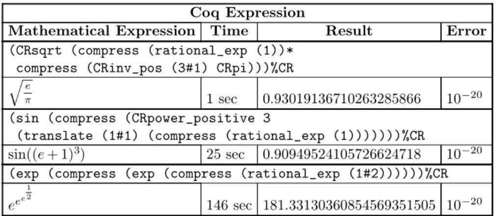
11.7 Timings . . . 95
11.8 Solving Strict Inequalities Automatically . . . 95
11.9 Remarks . . . 96
11.9.1 Using this Development . . . 96
11.9.2 Reworking Power Series . . . 97
11.9.3 Regular Functions vs Cauchy Sequences . . . 97
11.9.4 Haskell Prototype . . . 97
11.9.5 Comparisons With Other Implementations . . . 98
11.9.5.1 Comparison with Classical Reals . . . 99
12 Integration over R . . . 101
12.1 Informal Presentation of Riemann Integration . . . 101
12.1.1 Step Functions . . . 102
12.1.2 Step Functions Form a Monad . . . 104
12.1.3 Applicative Functors . . . 104
12.1.4 The Step Function Applicative Functor . . . 105
12.1.5 Two Metrics for Step Functions . . . 106
12.1.6 Integrable Functions and Bounded Functions . . . 108
12.1.7 Riemann Integral . . . 109
12.1.8 Stieltjes Integral . . . 110
12.1.9 Distributing Monads . . . 111
12.2 Implementation in Coq . . . 111
12.2.1 Glue and Split . . . 111
12.2.2 Equivalence of Step Functions . . . 112
12.2.3 Common Partitions . . . 112
12.2.4 Combinators . . . 113
12.2.5 Lifting Theorems . . . 114
12.2.6 The Identity Bounded Function . . . 115
12.2.7 Correctness . . . 116 12.2.8 Timings . . . 116 12.3 Remarks . . . 116 13 Compact Sets . . . 119 13.1 Product Metrics . . . 120 13.2 Hausdorff Metrics . . . 121 13.2.1 Finite Enumerations . . . 122
13.2.2 Mixing Classical and Constructive Reasoning . . . 123
13.3 Metric Space of Compact Sets . . . 123
13.3.1 Correctness of Compact Sets . . . 124
13.3.2 Distribution of FoverC . . . 126
13.3.3 Compact Image . . . 126
13.4 Plotting Functions . . . 127
13.4.1 Graphing Functions . . . 127
13.4.2 Rasterizing Compact Sets . . . 127
13.4.3 Plotting the Exponential Function . . . 127
13.5 Alternative Hausdorff Metric Definition . . . 128
13.6 Compactness and Computability . . . 129
13.6.1 A Constructive Approach to Filled Julia Sets . . . 132
14 Conclusion . . . 133 Bibliography . . . 135 Glossary of Symbols . . . 141 Index . . . 143 Samenvatting . . . 147 Curriculum Vitae . . . 151
List of Figures
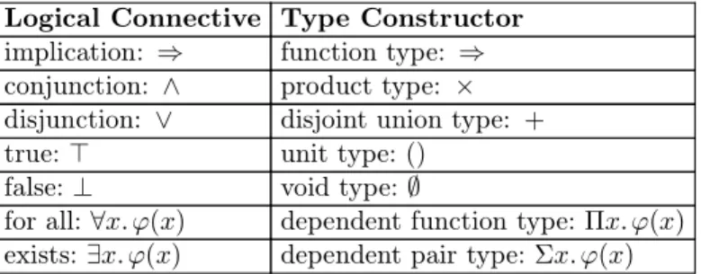
Verifying the trace of the computation of substitution in the case of∀y. ϕ. . . 35 Inductive definition of lazy natural numbers for Coq. . . 87 The Coq functioniterate_positeratesFa given number of times. . . 87 Given two step functions f and g, the step function f ⊲o⊳g is f squeezed into[0,o]and g
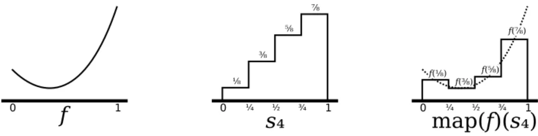
squeezed into[o,1]. . . 102 Given a uniformly continuous function f and a step function s4 that approximates the identity function, the step function map(f)(s4) (or fPs4) approximates f in the familiar Riemann way. . . . 109 A theorem in Coq stating that a plot on a 42 by 18 raster is close to the graph of the exponential function on[−6,1]. . . 128 One of these images represents the computable setK1
4+ǫ
, but which one? . . . 131
Chapter 1
Introduction
In the late nineteenth and early twentieth century, formal systems for mathemat-ical reasoning were developed by pioneers such as Frege [Frege, 1879], Russell, and Whitehead [Whitehead and Russell, 1925]. In principle all mathematical arguments could be written in some formal system and verifying the validity of these proofs would be a simple, but tedious, syntactic check. No person would want to engage in such a task, but modern computers excel at quickly performing simple, tedious tasks. Automated proof checkers have been developed that can quickly verify the validity of mathematical arguments that are written in their formal systems. Proof checkers are an ideal way of verifying mathematical arguments because they are fast and reliable. What remains difficult is converting standard mathematical arguments on paper into a formal language that is suitable for software verification. In a formal proof, no details of an argument can be omitted.
To aid people in the composition of formalized mathematics, proof assistants have been developed. These proof assistants contain an automated proof checker in the kernel of their code. The rest of the software supports the interactive development of formal proofs. They manage what goals remain to be proven and which assump-tions are available to prove those goals. They provide tools for automatically solving or reducing certain goals. However, even with all this assistance, creating formal proofs is a difficult and time consuming task for all but the simplest mathe-matical arguments. In this thesis I will develop some new tools that will lift some of this burden.
1.1 Main Topics and Contributions
This thesis is divided into two parts. In Part I, I discuss my development and veri-fication of the Gödel-Rosser incompleteness theorem, which I undertook in order to better understand the difficulties of creating formal proofs. This new formal proof is more general than the previous formal proof of the incompleteness the-orem [Shankar, 1994]. In Part II, using lessons learned about formalization from Part I, I develop a constructive theory of real numbers. This formalization extends previous work on constructive real analysis [Cruz-Filipe, 2004] by adding feasible evaluation of approximations of elementary real number expressions. The two parts are independent of each other and can be read separately. The theorems in this thesis have been developed and verified with the Coq proof assistant [The Coq Development Team, 2004].
1.1.1 Part I
I chose to verify the Gödel-Rosser incompleteness theorem because the proof is simple enough that it is covered in undergraduate mathematics courses, and I felt it was an extreme example of a mathematical proof whose details are omitted during its presentation. I tried to follow a traditional mathematical argument, and I mostly succeeded, but I learned that many of the traditional structures and argu-ments for this proof are difficult to encode in a formal proof. I have identified sev-eral aspects of the proof where non-traditional structures and arguments may be easier to use. Another lesson I learned is that one should spend time researching and thinking about how to simplify aspects of a proof before formalizing it. This pressure to invent more general data structures and proofs is a useful side effect of the formalization process.
1.1.2 Part II
In Part II, I develop a new approach to metric spaces. I define the completion of an arbitrary metric space, and I give detailed paper proofs of properties of my metric spaces. The paper proofs were written before formalization so that I could antici-pate difficulties and adjust definitions. I then develop the real numbers as the ana-lytic completion of the rationals and define common trigonometric operations on them. Because my data structures and functions have reasonable efficiency, the operations are feasible to execute. Formal proofs ensure that the operations are correct.
The primary purpose of developing a completion operation for metric spaces was to create an efficient real number implementation. However, the resulting completion operation is generic and can be used to complete other metric spaces. To illustrate this, I develop two other complete metric spaces: the completion of rational step functions, yielding integrable functions, and the completion of finite sets, yielding the compact sets.
The library I have developed could be used to create a scientific calculator that can evaluate real number expressions to arbitrary precision and guarantee that the results are correct. Furthermore, by using the theory of compact sets, one could create a graphing calculator with provably correct plots of functions. Because the computations are certified with formal proofs, the computations can be used inside proofs.
Using computation inside proofs is a powerful technique. The proof of the four colour theorem [Apple and Haken, 1976] and Kepler’s conjecture [Hales, 2002] both make heavy use of computation in their proofs. Verified computation is an essential ingredient needed to formalize these proofs. Gonthier has successfully used this technique to verify the four colour theorem with the Coq proof assistant [Gonthier, 2005]. I believe that my theory of real numbers provides the tools needed to verify Hales’s proof of the Kepler conjecture as well as other proofs that make use of real number computation, such as the disproof of Mertens conjecture [Odlyzko and teRiele, 1985]. More importantly, I believe the ideas in this part will prove useful for creating the next generation of effective implementations of constructive anal-ysis.
Chapter 2
Preliminaries
Constructive logic is usually presented as a restriction of classical logic where proof by contradiction and the law of the excluded middle are not allowed. However, con-structive logic can also be presented as an extension of classical logic.
Consider formulas constructed from universal quantification (∀), implication (⇒), conjunction (∧), true (⊤), false (⊥), and equality for natural numbers (=N).
Define negation using these primitives. Definition 2.1. ¬ϕ4ϕ⇒ ⊥.
We call a formula ϕstable when¬¬ϕ⇒ϕholds. One can (constructively) prove ϕ is stable for any formula ϕ generated from this set of connectives by induction on the structure of ϕ because m =N n is provably stable, and the connectives listed
above preserve stability. Thus, one can deduce classical results with constructive proofs for formulas generated from this restricted set of connectives.
This set of connectives is not really restrictive though; it can be used to define the other classical connectives.
Definition 2.2. Classical connectives:
ϕ∨˜ψ 4 ¬(¬ϕ∧ ¬ψ) ∃˜x. ϕ(x) 4 ¬(∀x.¬ϕ(x)).
With this full set of connectives, one can produce classical mathematics. The law of the excluded middle (ϕ∨˜ ¬ϕ)has a constructive proof when the classical disjunc-tion is used. As long as we have a stable goal we can do case analysis on the clas-sical disjunction.
Theorem 2.3. Assuming that ϕ ∨˜ ψ holds, we have ϕ⇒ θ and ψ⇒θ, and θ is stable, meaning ¬¬θ⇒θ, then θholds.
Proof. Because θ is stable, it is sufficient to prove that ¬¬θ holds. Assume that ¬θ holds. From this and the contrapositive of ϕ ⇒ θ we can conclude that ¬ϕ holds. Similarly ¬ψholds. But we have that ¬(¬ϕ∧ ¬ψ)holds from the definition of ϕ∨˜ψ. Thus we have a contradiction, as required.
We have a similar theorem for the classical existential.
Theorem 2.4. Assuming that ∃˜x. ϕ(x) holds, we have ∀x. ϕ(x) ⇒ θ, and θ is stable, meaning ¬¬θ⇒θ, then θholds.
Proof. Because θ is stable, it is sufficient to prove that ¬¬θ holds. Assume that ¬θ holds. From this and the contrapositive of ϕ(x) ⇒ θ we can conclude that ∀x.¬ϕ(x) holds. But we have that ¬(∀x.¬ϕ(x)) holds from the definition of ∃
˜x. ϕ(x). Thus we have a contradiction, as required.
So far, these two theorems can always be used because for any given formulaθ, we can prove¬¬θ⇒θ.
Now let us extend this logic by adding two new connectives, the constructive dis-junction (∨) and the constructive existential (∃). These new connectives come equipped with their constructive rules of inference given by natural deduc-tion [Thompson, 1991]. These constructive connectives are slightly stronger than their classical counterparts. Constructive excluded middle (ϕ ∨ ¬ϕ) cannot be deduced in general, and our inductive argument that¬¬ϕ⇒ϕholds no longer goes through if ϕ uses these constructive connectives. Therefore, statements such as
(¬ϕ⇒ ¬ψ)⇒(ψ⇒ϕ)are not general tautologies in constructive logic, but one can prove such statements when ϕis a stable formula.
We wish to use constructive reasoning because constructive proofs have a computa-tional interpretation. A constructive proof of ϕ∨ψ tells which of the two disjuncts hold. A proof of ∃n: N. ϕ(n) gives an explicit value for n that makes ϕ(n) hold. Most importantly, we have a functional interpretation of ⇒ and ∀. A proof of ∀n:N.∃m:N. ϕ(n, m) is interpreted as a function with an argumentn that returns anmpaired with a proof of ϕ(n, m).
The classical fragment also admits this functional interpretation, but formulas in the classical fragment typically end in ⇒ ⊥. These functions take their argu-ments and return a proof of false. Of course, there is no proof of false, so it must be the case that the arguments cannot simultaneously be satisfied. Therefore, these functions can never be executed. It turns out that only trivial functions such as this are created by proofs of classical formulas. This is why constructive mathe-matics aims to strengthen classical results. We wish to create proofs with non-trivial functional interpretations.
Constructive logic turns out to be compatible with classical logic. If one replaces the constructive existential and disjunction with their classical counterparts, then the resulting formula is a theorem if the original theorem was. In fact, the deduc-tive rules of construcdeduc-tive logic are a subset of the deducdeduc-tive rules of classical logic when connectives are reinterpreted this way. This means that constructive rea-soning can be understood by classical mathematicians, although classical mathe-maticians may find some of the reasoning unusual at times because they have a dif-ferent interpretation of the connectives.
Constructive mathematics is mathematics done with constructive logic. Some care needs to be taken when selecting the non-logical axioms to ensure that the compu-tational interpretation of the logic remains valid. Standard ZFC set theory used in mathematics implicitly assumes a classical logic, so it is not a useful choice; one would be essentially restricted to the classical portion of constructive logic. I will use a type theory called the calculus of (co)inductive constructions (CiC) [The Coq Development Team, 2004] as the mathematical foundation for this thesis. CiC adds inductive and coinductive data structures, such as natural numbers, lists, and streams, to constructive logic in a way that is compatible with the existing natural deduction style rules for constructive logic. In fact, most of the logical connectives are defined as inductive datatypes. Only (∀) remains primitive and (⇒) is defined as a special case of (∀) (see Section 2.2.2).
CiC is the foundation used by the Coq proof assistant, which is the system that I have used to verify the theorems in my thesis. I will attempt to present my work independent of any particular constructive foundation as much as possible so that the ideas can easily be transferred to other systems. However, I will make use of the notation from type theory in my presentation.
From now on, I will generally leave out the word “constructive” from phrases like “constructive disjunction” and “constructive existential” and simply write “dis-junction” and “existential”. This follows the standard practice in constructive math-ematics of using names from classical mathmath-ematics to refer to some stronger con-structive notion. I will explicitly use the word “classical” when I wish to refer to classical concepts. Rather than saying a statement is true in constructive logic, which suggests atrue/false dichotomy, I will say a statement holds or is proved. I may also say a statement is constructed, but I will usually reserve this term for constructive theorems outside the classical subset.
2.1 Dependently Typed Functional Programming
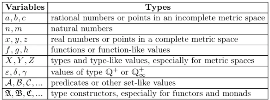
This computational interpretation of constructive deductions is given by the Curry-Howard isomorphism [Thompson, 1991]. This isomorphism associates formulas with dependent types, and proofs of formulas with functional programs of the associated dependent types. For example, the identity function λx:A. x of typeA⇒A repre-sents a proof of the tautologyA⇒A. Table 2.1 lists the association between logical connectives and type constructors.
Logical Connective Type Constructor implication: ⇒ function type: ⇒ conjunction: ∧ product type: × disjunction: ∨ disjoint union type: +
true:⊤ unit type:()
false:⊥ void type:∅
for all:∀x. ϕ(x) dependent function type:Πx. ϕ(x)
exists:∃x. ϕ(x) dependent pair type:Σx. ϕ(x)
Table 2.1. The association between formulas and types given by the Curry-Howard iso-morphism.
In dependent type theory, functions from values to types are allowed. Using types parametrized by values, one can create dependent pair types, Σx: A. ϕ(x), and dependent function types, Πx: A. ϕ(x). A dependent pair consists of a value x of typeA and a value of type ϕ(x). The type of the second value depends on the first value,x. A dependent function is a function from the typeAto the type ϕ(x). The type of the result depends on the value of the input.
The logical connectives and the type constructors from Table 2.1 mean the same thing, and I will use them interchangeably; however, I will usually prefer to use the logical connectives. Note that Coq has a sort of distinction between the two classes of connectives (see Section 2.3.2).
The association between logical connectives and types can be carried over to con-structive mathematics. We associate mathematical structures, such as the natural numbers, with inductive types in functional programming languages. We associate atomic formulas with functions returning types. For example, we can define equality on the natural numbers,x=Ny, as a recursive function:
0 =N0 4 ⊤ S(x) =N0 4 ⊥
0 =NS(y) 4 ⊥ S(x) =NS(y) 4 x=Ny
One catch is that general recursion is not allowed when creating functions. The problem is that general recursion allows one to create a fixed point operator fix : (ϕ⇒ϕ)⇒ϕthat corresponds to a proof of a logical inconsistency. To prevent this, we allow only well-founded recursion over an argument with an inductive type. Because well-founded recursion ensures that functions always terminate, the lan-guage is not Turing complete. However, one can still express fast-growing func-tions, such as the Ackermann function, without difficulty by using higher-order functions [Thompson, 1991].
Because proofs and programs are written in the same language, we can freely mix the two. For example, I will represent the real numbers (see Definition 9.16 and Definition 11.1) by the type
∃f:Q+
⇒Q.∀ε1ε2.|f(ε1)−f(ε2)| ≤ε1+ε2. (2.1)
A value of this type is a pair of a function f: Q+ ⇒ Q and a proof of
∀ε1ε2.|f(ε1)−f(ε2)| ≤ε1+ε2. The idea is that a real number is represented by a
function f that maps any requested precisionε:Q+ to a rational approximation of the real number. Not every function of type Q+ ⇒ Q represents a real number. Only those functions that have coherent approximations should be allowed. The proof object paired with f witnesses the fact that f has coherent approximations. This is one example of how mixing functions and formulas allows one to create pre-cise datatypes.
2.1.1 Evaluation
This computational interpretation of constructive mathematics is more than a nice theoretical feature. The algorithms contained inside constructive proofs can actu-ally be executed inside the type theory. One can view this as part of Bishop’s pro-gram to see constructive mathematics as a propro-gramming language. For example, the expression 2 + 2 and the expression 4 are considered equivalent. They can be substituted for each other in any context, and the system will evaluate (2 + 2)to 4 when necessary.
A technique called reflection [Barendregt and Geuvers, 2001] uses this evaluation mechanism to allow one to create proofs by using computation. One example of this technique is used in Section 11.4.2 to prove the correctness of my definition of π. Thus the computational and logical parts of type theory enhance each other. Correct algorithms can be used to create proofs, and proofs verify the logical cor-rectness of algorithms.
2.1.2 Formalizing Mathematics with a Computer
There are several different approaches to formalizing mathematics on a com-puter [Wiedijk, 2006]. Often people use a system that provides classical logic. Many systems implement classical higher-order logic, such as HOL Light, Isabelle/HOL, and PVS. A few systems implement classical set theory, such as Mizar and Isabelle/ZF.
One of the main benefits of formalizing mathematics with a computer, aside from providing high assurance of correctness, is the ability for the computer to automate reasoning that would be too tedious to formalize by hand. This automated rea-soning can range from the mundane, automatically differentiating an expression, to the extreme, the huge case analysis needed in the four colour theorem [Gonthier, 2005].
Systems based on classical logic must perform this computation outside the logic, whereas a constructive system, such as Coq, can perform computation both on the outside, as Coq does with its tactic system, and on the inside, as Coq does with its evaluation mechanism.
To prove the correctness of an algorithm using a classical system, generally one writes out the function first. Once the function is defined, one can use classical rea-soning to prove properties about that function. In a constructive system, one has the option to mix proofs into the definition of the function. This allows one to prove properties of a function as the function is defined. However, one still has the option of writing the function first and then reasoning about it.
One can see the classical approach to correctness as taking a constructive theorem and Skolemizing the constructive existentials (and constructive disjunctions). The functions one initially writes become the instances of the Skolem functions in the transformed theorem. The resulting theorem is in the classical fragment of con-structive logic and classical arguments can be used to prove it.
I do not believe that there is anything to be gained by forcing a separation between the (classical) logical aspects and the algorithmic aspects when proving properties of algorithms. Sometimes this separation is a useful way to proceed, but usually the “flow” of the proof follows the “flow” of data in the algorithm. It makes sense to attach proof objects to values inside the algorithm, particularly when one wants to express an invariant of a datatype. I feel working with data and proofs together clarifies the development of algorithms and makes proving properties easier. Some-times one wants to prove a property of how two or more functions interact; for example, when proving one function distributes over another. In this case, it is usu-ally best to provide a proof separate from either function.
When working in a constructive system, one has the option to avoid algorithmic development entirely and simply write a constructive proof. By its constructive nature, this proof can be executed to compute constructive witnesses. However, if no attention is paid to the construction, the resulting algorithms are often ineffi-cient. Therefore, it is wise to think of creating a constructive proof as a program-ming task as well as a mathematical task. One should take the same algorithmic considerations into account that one would when writing any other functional pro-gram.
2.2 A Brief Introduction to Type Theory
Types in type theory are similar to sets in set theory in that they are a collection of values. One important difference between type theory and set theory is that in type theory every value belongs to a unique type. I write a: A when a value a belongs to a type A. This means that the natural number 1N:N is distinct from
the rational number 1Q:Q because they belong to different types. However, I will
often just write1 and leave the distinction implicit. Values are also called “objects”; the two terms are synonymous.
Quantifiers always range over some type; for example,∀x:N.x= 0∨ ∃y:N.x=S(y). Sometimes I will omit writing the type for the quantified variable when it is clear from context.
One can form new types from existing types. Given typesA and B, one can create the disjoint union type,A+B, the Cartesian product type, A×B, and the type of functions from A to B, A⇒B. These types are the same as the logical connectives (∨), (∧), and (⇒) respectively. The functions π1:A×B⇒A and π2:A×B⇒B
are the first and second projection functions of the Cartesian product type.
In type theory, proofs are objects, and propositions are types. This is known as the propositions-as-types interpretation. Propositions are types whose objects consist of all of their proofs. Therefore, one writes p: ϕ when p is a proof of ϕ. When a proposition has no proofs, it has no members. Thus it is the inhabited propositions that are the valid propositions. Propositions are also values that belong to the type of propositions. In Coq, the type of propositions is called Prop (see Section 2.3.2); however I will denote this type as ⋆ and writeϕ:⋆. Predicates can be seen as func-tions whose codomains are proposifunc-tions. For example, predicates over the natural numbers will have the typeN⇒⋆.
2.2.1 Inductive types
CiC has inductive and coinductive types, so standard inductive types such as Booleans, natural numbers, integers, lists, binary trees, etc. are available as well as coinductive types such as infinite streams. I will use standard mathematical nota-tion for such types.
A record is an inductive data type that has only one constructor. Coq has special notation for defining records that allows one to create the inductive type and the projection functions for its fields at the same time.
A value of an inductive data type can be consumed by a structurally recursive function. These recursive functions can be evaluated inside type theory as men-tioned in Section 2.1.1.
In addition to inductive types, inductive type families (also called inductive predi-cates) can be defined. In this case, the inductive definition produces not a type but a predicate. See Section 4.4 for an example of an inductively defined type family.
2.2.2 Constructive Functions
In classical mathematics, a classical function is a type of binary relation F satis-fying the property
(∀x.∃˜y.F(x, y))∧(∀xyz.F(x, y)∧F(x, z)⇒y=z).
In constructive mathematics, a (constructive) function is a value of type A⇒ B, where ⇒ is a primitive connective. This ⇒ connective used in the function type is identical to the implication logical connective. In type theory, values of this con-structive function type are formed by specifying how the output is constructed from the input, usually using a lambda expression (see Section 2.2.4). Constructive functions can be evaluated internally in type theory as mentioned in Section 2.1.1. Additionally there is the dependent function type, written ∀a: A. B(a), which is identical to the universal quantifier. In this case the codomain of the function can depend on the input parameter. Like the regular function type, values of a depen-dent function type are specified by lambda expressions and can be evaluated inter-nally in type theory. In fact, A⇒B is simply notation for ∀a:A.B where B does not depend ona.
2.2.3 Curried Functions
A multi-argument function in mathematics is typically represented as a function whose domain is a Cartesian product. For example, a binary function would have the type A × B ⇒ C. It is traditional in functional programming to use curried functions. A curried binary function has type A⇒B⇒C (meaningA⇒(B⇒C)
by the usual associativity rule for ⇒), which can easily be shown to be isomorphic to A×B⇒C. When applying a curried binary function it would be more techni-cally accurate to write f(a)(b), but for clarity I will sometimes write f(a, b) as if the function were not curried.
2.2.4 Anonymous Functions
I will on occasion use anonymous functions. Anonymous functions—common in functional programming—are declared using the λsymbol. For example, the recip-rocal function can be written as λx.x−1 and can be applied to arguments, as in
λx.x−12
3
is equal to 32.
2.2.5 Extensional Equality
In this thesis I will use the equality sign (=) for extensional equality. Two func-tions f , g of the same type are considered extensionally equal when, for any input given to both functions, the outputs of the functions are extensionally equal:
f=g4∀a. f(a) =g(a)
Two values of an inductive type are extensionally equal when their constructors are the same and all parameters are extensionally equal.
Extensional equality is the finest equality we will need in my thesis. However, Coq uses a finer equality called intensional equality (see Section 2.3.1) for its funda-mental equality.
Another sort of equality that we will frequently use is setoid equality (see Sec-tion 2.2.8), which is generally coarser than extensional equality.
2.2.6 No Subtypes
Coq does not have subtyping.2.1 This means thatZ cannot be considered as a
sub-type of Q. Functions, usually injections, are instead used to change data from one type to the other type. Coq has a coercion mechanism that will automatically infer many of these injections and hide the injections from being printed. Defining a coercion fromZtoQallows one to use values of Zas if they were values ofQ.
2.2.7 Predicates Instead of Sets
Sets do not exist as such in type theory. Usually sets are replaced by predicates over a particular type. For example, subsets of the natural numbers are identified with N⇒⋆, predicates on the natural numbers. A value xsatisfies a predicate P when P(x) is an inhabited type. Often I will use set theoretic notation to denote membership of a predicate:
x∈P 4 P(x)
∀x∈P .ϕ 4 ∀x.P(x)⇒ϕ ∃x∈P .ϕ 4 ∃x.P(x)∧ϕ
Similar quantifier notation will be used for inequalities such as ∀i < n. ϕ and ∃i≥n. ϕ.
2.1. Technically, Coq has subtyping in its universe levels, but we will not concern ourselves with universe levels in this thesis.
2.2.8 Setoids Instead of Quotients
A quotient type is a type modulo a given equivalence relation on that type. For instance, the type Q is often considered as a quotient of the type Z× N+. CiC does not have quotient types. One instead passes around the equivalence relation in question. To do this, one often uses a data structure called a setoid. A setoid
(A, ≍A) is a type paired with an equivalence relation on that type. Functions
between setoids that preserve their equivalence relations are called respectful. Proving that a function is respectful consists of the same work in traditional math-ematics needed to prove that a function over quotients is well-defined. Respectful functions are also calledmorphisms.
2.2.8.1 Rewrite Automation
Coq has special support for reasoning about setoids through its setoid_rewrite and setoid_replace tactics [Coen, 2004]. These tactics will automatically create the deductions for substitution of setoid equivalent terms into respectful functions and relations. This support makes reasoning about setoid equivalence almost as easy as reasoning about equality in Coq.
Furthermore, Coq has the ability to define a database of rewrite lemmas. These lemmas have terms of the form a≍Ab for their conclusions. When they are added
to the database the user indicates which way substitution should be performed (the same lemma can be added to different databases with different directions). The user can then use the database as a rewrite system to process a hypothesis or goal. The autorewrite <database> tactic will repeatedly try to use the lemmas in the
named database to rewrite the goal. Well crafted rewrite databases can be used to quickly transform or simplify expressions.
2.2.9 Apartness Instead of “Not Equal”
In analysis, when considering Hausdorff spaces, it is often the case that being “not equal” is a non-stable atomic formula [Bauer and Taylor, 2008]. However, x y is notation for ¬x=y, and it is always stable. Therefore, constructive analysis uses a relation called apartness, written x#y, which is not necessarily stable. For example, the apartness relation for real numbers,x#y4x < y∨y < x, is not prov-ably stable. In these cases ac-setoid (a constructive setoid) data structure is often used instead of a setoid. A c-setoid(A,#A)is a type paired with an apartness
rela-tion. In this case, arespectful function from a c-setoid Ato a c-setoid B, is a func-tionf:A⇒B such that ∀x, y:A. f(x)#Bf(y)⇒x#Ay.
2.2.10 Classical Propositions Have One Proof
All classical propositions have at most one proof, meaning that if p:ϕand q:ϕ are two proof objects of the same classical proposition ϕ, then we can prove that pand q are (extensionally) equal, p=q. In general, I will denote all the unique proofs of classical propositions as∗ (e.g. ∗:⊤and∗:⊥ ⇒ϕ).
2.2.11 Omitted Parameters
Throughout this thesis there are many places where I formally need to provide proofs of propositions as arguments to functions. However, to allow for a clearer presentation, I will usually omit these parameters. For example, the logarithm on rational numbers, lnQ(a), requires a proof object showing that0<Qa, but I do not
show this parameter (see Section 11.4).
2.3 Coq Specific Issues
The previous section detailed the properties of the type theory I will be informally working in for this thesis. Although I made reference to the Coq system at times, the type theory I describe is fairly generic and should be easily adapted to work in many different implementations of type theory. However, my formal work has been done in the Coq proof assistant, so below I address some specific properties of Coq that are relevant to my formalization.
2.3.1 Intensional Equality
In type theory, functions are represented by the program that does the computa-tion. In Coq, two functions can only be proven equal if after normalization they are the same program. This means that if two functions are extensionally equal, they may not be intensionally equal in Coq.
For inductive data types without functions as parameters to constructors, inten-sional equality coincides with exteninten-sional equality, so much of the time this distinc-tion does not matter. On those occasions where I need to deal with extensional equality between functions in Coq, I can often just expand out the definition of extensional equality. Thus, rather than trying to prove f = g, I prove ∀a. f(a) =g(a)instead.
2.3.2
Prop
versus
Set
The Coq system has a special universe calledProp. The Prop universe is like ⋆ in that it has types as members. The regular type universe is called Setand also has types as members, like ⋆.2.2 These two universes behave largely the same. Both
universes have inductive types and function/implication types. When defining an inductive type, one specifies which universe the inductive type will inhabit. Func-tions in both universes can be evaluated inside Coq, as long as the funcFunc-tions are not opaque (see Section 2.3.3).
2.2. There is also an infinite number of universe levels containingSetandProp, but we can safely
ignore this for our needs.
Generally the two universes serve to divide up types that are otherwise identical according to whether their values are intended to play a logical or functional role (recall Table 2.1). For each entry in Table 2.1, Coq has at least two operators, one for the logical side and one for the functional side. For example, Coq has one pro-duct for logical conjunction and another propro-duct for propro-duct types. Inpro-ductive types for both universes can have parameters whose types belong to either universe. In this way types from both universes can be mixed together. The only major differ-ence between thePropandSetuniverses is in the way that case analysis for induc-tive types behave. Case analysis on an inducinduc-tive type from thePropuniverse is not allowed to result in a value in the Set universe. This prevents information from flowing from the Propuniverse to the Set universe. This restriction allows Coq to optimize program extraction by throwing away all values from the Prop universe during program extraction [Paulin-Mohring, 1989]. This is safe because the case analysis restriction means that no value from the Set universe can depend on choices made in thePropuniverse.
There is an important exception to this case analysis rule. For the special case of inductive types declared in the Prop universe that have at most one constructor whose parameters are all from the Prop universe, case analysis is allowed to return values in the Set universe. Case analysis is safe in this instance because inductive types with at most one constructor provide no information; There will be only one branch in the case analysis. During program extraction, the case analysis is simply replaced by the code of this one branch. Since all the parameters are from theProp universe, no parameters from the case analysis will occur in the code extracted from the one branch.
Generally I only put inductive types in theProp universe if they satisfy this special condition.2.3 This allows me to enjoy unrestricted case analysis and still allow for
efficient program extraction.
I will not be making a Prop/Set distinction in my general discussion; however, I may refer to it when making comments specifically about the Coq implementation.
2.3.3 Opaque Objects
Theorems and definitions can be marked as opaque in Coq. Opaque definitions cannot be unfolded during computation. In this sense they behave much like axioms in Coq. Generally I make all objects in theProp universe opaque and leave all objects in the Set universe as transparent. This usually works well because I ensure that all my objects from the Prop universe have no information (see Sec-tion 2.3.2).
2.3. There are some cases when I would put inductive type families inProp, even if they have mul-tiple constructors. However, all inductive type families in this thesis will be put in theSet uni-verse.
One notable exception to making all Prop objects opaque would be a proof that a relation is well-founded. Even though the accessibility predicate is in the Prop uni-verse and satisfies the one constructor rule given in Section 2.3.2, it generally needs to be transparent so that well-founded induction over the relation can proceed. The other notable exception is that proofs of equality occasionally need to be trans-parent to allow “safe type-casts”2.4to be evaluated.
Declaring objects as opaque is useful because it can prevent computation from expanding irrelevant definitions during evaluation. This is so useful that Coq also has a mechanism to temporarily mark certain definitions as opaque and make them transparent again later.
2.3.4 Coq Notation
On occasion I will use Coq’s concrete syntax to clearly specify the formal theorems I have proven. For those not familiar with Coq syntax, here is a short list of nota-tion.
• ->,/\,\/, and ~are the logical connectives⇒,∧, ∨, and¬.
• A + B, A * B, and A -> B form disjoint union types, Cartesian product types, and function types.
• *, +, and S are the arithmetic operations of multiplication, addition, and successor.
• inl and inr are the left and right injection functions of types A -> A + B andB -> A + B.
• ::, and++are the list operations cons and append. • _is an omitted parameter that Coq can infer itself.
Function application is indicated by juxtaposition. Thus f(x) is written simply as f xin Coq. For more details see the Coq 8.0 reference manual [The Coq Develop-ment Team, 2004].
2.4. A safe type-cast allowsa:Ato be transformed into a value of typeB when given a proof of
A=B.
Part I
Chapter 3
Introduction
In this part, I discuss my formal proof of the Gödel-Rosser incompleteness theorem for arithmetic. The proof shows that any complete first-order theory of a suitable axiom system using only the symbols +, ×, 0, S, and < is inconsistent. The
axiom system must contain the nine axioms of a system called NN. These nine axioms define the five symbols. The axiom system must also be expressible in itself. This restriction prevents the incompleteness theorem from applying to axioms sys-tems such as the true first order sentences inN. Finally, the axiom system must be decidable, so that it is constructively decidable what is and is not a proof. This restriction is subtly, but significantly, different from requiring the axiom system to be computable. The difference is discussed later in Section 6.1.
A computer-verified proof of Gödel’s incompleteness theorem is not new. In 1986 Shankar created a proof of the incompleteness of Z2, hereditarily finite set theory, in the Boyer-Moore theorem prover [Shankar, 1994]. My work is the first computer-verified proof of the essential incompleteness of arithmetic. Harrison recently com-pleted a proof in HOL Light [Harrison, 2000] of the essential incompleteness of Σ1
-complete theories, but has not shown that any particular theory isΣ1-complete.
My proof was developed and checked in Coq 7.3.1 using Proof General under XEmacs. It is part of the user contributions to Coq and can now be checked in Coq 8.0 [The Coq Development Team, 2004]. Examples of source code in this docu-ment use the new notation introduced in Coq 8.0.
This part points out some of the more interesting problems I encountered formal-izing the incompleteness theorem. My proof loosely follows the presentation of incompleteness given in my undergraduate logic textbook, An Introduction to Mathematical Logic by Hodel [Hodel, 1995]. I use a more standard Hilbert-style deduction system rather than the one defined by Hodel. I referred to the supple-mentary text for the book Logic for Mathematics and Computer Science [Burris, 1997] to construct Gödel’s β-function, and I take some inspiration from Shankar’s work as described in Metamathematics, Machines, and Gödel’s Proof [Shankar, 1994]. I also use Caprotti and Oostdijk’s contribution of Pocklington’s criterion [Caprotti and Oostdijk, 2001] to prove the Chinese remainder theorem. My proof is entirely constructive.
In this part, I first discuss my formalization of first-order classical logic over an arbitrary language (Chapter 4). This is followed by the definition of an axiom system called NN and the axiom system for Peano arithmetic. Then I discuss coding formulas and proofs as natural numbers followed by a discussion about primitive recursive functions operating on these codes (Chapter 5). Next I give the statement of the essential incompleteness of NN (Chapter 6). I discuss the fixed point theorem, Rosser’s incompleteness theorem, and the incompleteness of Peano arithmetic. Finally, I give some general remarks about my experience and how to extend my work in order to formalize Gödel’s second incompleteness theorem (Chapter 9.5).
This part is an expansion of my publication, “Essential Incompleteness of Arith-metic Verified by Coq” [O’Connor, 2005a].
Chapter 4
First-Order Classical Logic
The first step to prove the incompleteness theorem is to develop a theory of first order logic inside Coq. In essence Coq’s logic is a formal metalogic to reason about this internal logic. I created inductive types of well-formed terms and formulas parametrized over a first order language. I then created an inductive definition of Hilbert-style deductions for classical logic.
I make essential use of Coq’s dependent type system. Terms and Formulas are types that depend on the language. Also, dependent types are used in the defini-tion of funcdefini-tion and reladefini-tion symbols so that the type system enforces that all terms and formulas be well-formed. This approach differs from Harrison’s definition of first order terms and formulas in HOL Light [Harrison, 1998a] because HOL Light does not have dependent types.
4.1 Data Structures for
Language
I defined Language to be a dependent record of types for symbols and an arity function from symbols toN. The Coq code is:
Record Language : Type := language {Relations : Set;
Functions : Set;
arity : Relations + Functions -> nat}.
In retrospect it would have been slightly more convenient to use two arity functions instead of using the disjoint union type.
The entire development of first-order logic is parametrized over this structure by using Coq’s section mechanism.
4.2 Data Structures for
Term
and
Formula
For any language, a Term is either a variable indexed by a natural number or a function symbol plus a list of n terms where n is the arity of the function symbol. My first attempt at writing this in Coq failed.
Variable L : Language. (* Invalid definition *) Inductive Term0 : Set := | var0 : nat -> Term0
| apply0 : forall (f : Functions L) (l : List Term0), (arity L (inr _ f))=(length l) -> Term0.
Some people may think that the occurrence of the List Term0 type in apply0 causes Coq to reject this definition; however, this is actually not problematic. It is the type (arity L (inr _ f))=(length l) that fails to meet Coq’s positivity requirement for inductive types. Expanding the definition of length reveals a hidden occurrence of Term0 which is passed as an implicit argument to length. It is this occurrence that violates the positivity requirement.
My second attempt met the positivity requirement, but it had other difficulties. First, one creates the well-known inductive family of types lists of length n, usually calledVector.
Inductive Vector (A : Set) : nat -> Set := | Vnil : Vector A 0
| Vcons : forall (a : A) (n : nat), Vector A n -> Vector A (S n). Using this I could have definedTermas follows. Variable L : Language.
Inductive Term1 : Set := | var1 : nat -> Term1
| apply1 : forall f : Functions L,
(Vector Term1 (arity L (inr _ f))) -> Term1.
My difficulty with this definition was that the induction principle generated by Coq is too weak to work with. The generated induction principleTerm1_indis:
Term1_ind
: forall P : Term1 -> Prop, (forall n : nat, P (var1 n)) -> (forall (f : Functions L)
(v : Vector Term1 (arity L (inr (Relations L) f))), P (apply1 f v)) -> forall b : Term1, P b.
Term1_indrequires showing P (apply1 f v) for all fandv without any inductive hypothesis about v. If, for instance, one wants prove that a particular variable is not used in a term, one will need to verify that this holds for each term in the vector v; however, the inductive hypothesis for each term of the vector v is not available.
Instead I created two mutually inductive types:TermandTerms. Variable L : Language.
Inductive Term : Set := | var : nat -> Term
| apply : forall f : Functions L, Terms (arity L (inr _ f)) -> Term with Terms : nat -> Set :=
| Tnil : Terms 0
| Tcons : forall n : nat,
Term -> Terms n -> Terms (S n).
Again the automatically generated induction principle is too weak, but theScheme command generates suitable mutual-inductive principles. For example, the com-mand
Scheme Term_Terms_rec := Minimality for Term Sort Set with Terms_Term_rec := Minimality for Terms Sort Set. generates a term of the following type.
Term_Terms_rec
: forall (P : Set) (P0 : nat -> Set), (nat -> P) ->
(forall f : Functions L,
Terms (arity L (inr (Relations L) f)) -> P0 (arity L (inr (Relations L) f)) -> P) -> P0 0 ->
(forall n : nat, Term -> P -> Terms n -> P0 n -> P0 (S n)) -> Term -> P.
In this case we have two “result” types. P is the result of evaluating onTerm, while P0is the result of evaluation onTerms.
The disadvantage of this approach is that useful lemmas about Vectors must be reproved for Terms. Some of these lemmas are quite tricky to prove because of the dependent type. For example, proving forall x : Terms 0, Tnil = x is surpris-ingly difficult.
It turns out that the Term1 definition would have been adequate. One can explic-itly make a sufficient induction principle by using nested Fixpoint functions [Marche, 2005].
Section RecursionDef. Variable P : Set.
Variable P0 : nat -> Set. Variable varcase : nat -> P. Variable applycase :
forall f : Functions L, Vector Term1 (arity L (inr _ f)) -> P0 (arity L (inr _ f)) -> P.
Variable nilcase : P0 0. Variable conscase :
forall n : nat, Term1 -> P -> Vector Term1 n -> P0 n -> P0 (S n). Fixpoint Term1_rec_new (t : Term1) : P :=
let fix Terms1_rec (n : nat)(vec : (Vector Term1 n)) {struct vec} : P0 n :=
match vec in (Vector _ n) return (P0 n) with | Vnil => nilcase
| Vcons term m terms =>
conscase m term (Term1_rec_new term) terms (Terms1_rec m terms) end
in
match t with
| var1 n => varcase n
| apply1 f terms => applycase f terms (Terms1_rec _ terms) end.
End RecursionDef.
I would recommend using something like theTerm1 definition with Term1_rec_new in future work.
The definition ofFormula was straightforward. Inductive Formula : Set :=
| equal : Term -> Term -> Formula
| atomic : forall r : Relations L, Terms (arity L (inl _ r)) -> Formula
| impH : Formula -> Formula -> Formula | notH : Formula -> Formula
| forallH : nat -> Formula -> Formula.
I defined the other logical connectives in terms ofimpH,notH, and forallH. Definition orH (A B : Formula) := impH (notH A) B.
Definition andH (A B : Formula) := notH (orH (notH A) (notH B)). Definition iffH (A B : Formula) := andH (impH A B) (impH B A). Definition existH (x : nat) (A : Formula) :=
notH (forallH x (notH A)).
The equals relation is part of the definition of Formula, so it does not occur as a relation symbol in the language. The natparameter of forallHis the index of the variable being quantified. The Terms parameter occurring in atomic would be replaced with (Vector Term1) if the definition of Term1 were used. The H at the end of the logic connectives, such asimpH, stands for “Hilbert” and is used to distin-guish them from Coq’s connectives.
For example, the formula¬∀x0.∀x1.x0 =x1is represented by:
notH (forallH 0 (forallH 1 (equal (var 0) (var 1))))
There are two common alternatives to handle variable binding. One alternative is to use higher order abstract syntax to handle bound variables by giving forallH the type (Term -> Formula) -> Formula. I would represent the above example as:
notH (forallH (fun x : Term =>
(forallH (fun y : Term => (equal x y)))))
This technique would require additional work to disallow “exotic terms” that are created by passing a function into forallH that does a case analysis on the term and returning entirely different formulas in different cases. Despeyroux and Hirschowitz [Despeyroux and Hirschowitz, 1994] address this problem by creating a complicated predicate that only valid formulas satisfy. Recently, Chlipala [Chlipala, 2008] has created an elegant solution for using higher order abstract syntax.
Another alternative is to use de Bruijn indices to eliminate named variables. How-ever dealing with free and bound variables with de Bruijn indices can be diffi-cult [McBride and McKinna, 2004a].
Using named variables allowed me to closely follow the standard way of writing for-mulas in mathematics. Using named variables is also helpful to persuade people of the correctness of the statement of the incompleteness theorem, which refers to the notion of provability and hence formulas.
Renaming bound variables turned out to be a constant source of work during devel-opment, because variable names and terms were almost always abstract. In prin-ciple the variable names could conflict, so it was constantly necessary to consider this case and deal with it by renaming a bound variable to a fresh one. Perhaps it would have been better to use de Bruijn indices and a deduction system that only deduced closed formulas, or perhaps one of the alternative implementations of vari-ables that I discuss in Section 7.7.
4.3 Definition of
substituteFormula
I defined the function substituteFormulato substitute a term for all occurrences of a free variable inside a given formula. While the definition ofsubstituteTerm is simple structural recursion, substitution for formulas is complicated by quantifiers. Suppose we want to substitute the term s for xi in the formula ∀xj. ϕ and i j. Supposexj is a free variable of s. If we naïvely perform the substitution, then the
occurrences of xj in sget captured by the quantifier. One common solution to this
problem is to disallow substitution for a termswhen sis not substitutable forxiin
ϕ. The solution I took was to rename the bound variable in this case:
(∀xj. ϕ)[xi/s]4 ∀xk.(ϕ[xj/xk])[xi/s]wherekiandxkis not free inϕors
Unfortunately this definition is not structurally recursive. The second substitution operates on the result of the first substitution, which is not structurally smaller than the original formula. Coq will not accept this recursive definition as is; it is necessary to prove the recursion will terminate. I proved that substitution preserves the depth of a formula, and that each recursive call operates on a formula of smaller depth.
One of McBride’s mantras says, “If my recursion is not structural, I am using the wrong structure” [McBride, 1999, p. 241]. In this case, my recursion is not struc-tural because I am using the wrong recursion. Stoughton shows that it is easier to define substitution that substitutes all variables simultaneously because the recur-sion is structural [Stoughton, 1988]. If I had used this definition, I could have defined substitution of one variable in terms of it and many of my difficulties would have disappeared.
4.4 Definition of
Prf
I defined the inductive type(Prf Gamma phi) to be the type of proofs ofphi, from the list of assumptions Gamma. Originally (Prf Gamma phi) was a member of the Prop universe. It seemed natural to considerΓ⊢ϕas a proposition, but it is impor-tant in this work to be able to distinguish between different proofs of the same statement. To get the ability to distinguish between different proofs requires that (Prf Gamma phi)be inSet.
Inductive Prf : Formulas -> Formula -> Set := | AXM : forall A : Formula, Prf (A :: nil) A
| MP : forall (Axm1 Axm2 : Formulas) (A B : Formula), Prf Axm1 (impH A B) -> Prf Axm2 A ->
Prf (Axm1 ++ Axm2) B
| GEN : forall (Axm : Formulas) (A : Formula) (v : nat), ~ In v (freeVarListFormula L Axm) -> Prf Axm A ->
Prf Axm (forallH v A)
| IMP1 : forall A B : Formula, Prf nil (impH A (impH B A)) | IMP2 : forall A B C : Formula,
Prf nil (impH (impH A (impH B C))
(impH (impH A B) (impH A C))) | CP : forall A B : Formula,
Prf nil (impH (impH (notH A) (notH B)) (impH B A)) | FA1 : forall (A : Formula) (v : nat) (t : Term),
Prf nil (impH (forallH v A) (substituteFormula L A v t)) | FA2 : forall (A : Formula) (v : nat),
~ In v (freeVarFormula L A) -> Prf nil (impH A (forallH v A)) | FA3 : forall (A B : Formula) (v : nat),
Prf nil
(impH (forallH v (impH A B))
(impH (forallH v A) (forallH v B))) | EQ1 : Prf nil (equal (var 0) (var 0)) | EQ2 : Prf nil (impH (equal (var 0) (var 1))
(equal (var 1) (var 0))) | EQ3 : Prf nil
(impH (equal (var 0) (var 1))
(impH (equal (var 1) (var 2)) (equal (var 0) (var 2)))) | EQ4 : forall R : Relations L, Prf nil (AxmEq4 R)
| EQ5 : forall f : Functions L, Prf nil (AxmEq5 f).
AxmEq4 and AxmEq5 are recursive functions that generate the equality axioms for relations and functions. AxmEq4 Rgenerates
x0= x1⇒ ⇒ x2n−2= x2n−1 ⇒(R(x0,x2,,x2n−2)⇔ R(x1,x3,,x2n−1)) andAxmEq5 fgenerates
x0 = x1⇒ ⇒ x2n−2= x2n−1⇒ f(x0,x2,,x2n−2)= f(x1,x3,,x2n−1) I found that replacing ellipses from informal proofs with recursive functions was one of the most difficult tasks. This case was easy, but in general, the informal proof does not contain information on what inductive hypothesis should be used when reasoning about these recursive definitions. Figuring out the correct inductive hypotheses was not always easy.
4.5 Definition of
SysPrf
There are some problems with the definition of Prf given. It requires the list of axioms to be in the correct order for the proof. For example, if we have Prf Gamma1 (impH phi psi) and Prf Gamma2 phi then we can conclude only Prf Gamma1++Gamma2 psi. We cannot conclude Prf Gamma2++Gamma1 psior any other permutation of the axioms. If an axiom is used more than once, it must appear in the list more than once. If an axiom is never used, it must not appear. Also, the number of axioms must be finite because they form a list.
One possible solution would be to add permutation, weakening, and contraction rules for axioms to the inductive definition of Prf. However, this would further complicate the definition of Prf, which we would like to keep as simple as possible, and it would still not allow the number of axioms to be infinite. To solve this problem, I instead defined System to be Ensemble Formula and SysPrf T phi to be the proposition that the systemTprovesphi.
Definition System := Ensemble Formula. Definition mem := Ensembles.In.
Definition SysPrf (T : System) (f : Formula) : Prop := exists Axm : Formulas,
(exists prf : Prf Axm f,
(forall g : Formula, In g Axm -> mem _ T g)).
The type Ensemble A represents subsets of A by predicates of type A -> Prop. Recall that a : A is considered to be a member of T : Ensemble A if and only if the type T a is inhabited. I also defined mem to be Ensembles.In so that it does not conflict withList.In.
The separation between the notions of Prf and SysPrf is useful. Each member of Prf is a finite value that can easily be encoded by a natural number (see Sec-tion 5.1), whileSysPrfallows one to work with infinite axiom systems.
4.6 The Deduction Theorem
The deduction theorem states that if Γ ∪ {ϕ} ⊢ ψ then Γ ⊢ ϕ ⇒ ψ. In Coq its formal statement is:
Theorem DeductionTheorem :
forall (T : System) (f g : Formula) (prf : SysPrf (Add _ T g) f), SysPrf T (impH g f).
There is a choice of whether the side condition for the ∀-generalization rule, ~In v (freeVarListFormula L Axm), should be required or not. If this side con-dition is removed, then the deduction theorem requires a side concon-dition on it. Usu-ally all the formulas in an axiom system are closed, so the side condition on the∀ -generalization is easy to show. I therefore decided to keep the side condition on the ∀-generalization rule.
Originally my proof of the deduction theorem relied on an assumption that the lan-guage is decidable, meaning that the function and relation symbols form decidable types.
• forall x y : Functions L, {x=y} + {x<>y} • forall x y : Relations L, {x=y} + {x<>y}
The classical proof of the deduction theorem at one point considers whether ϕ∈F or ϕ F for a finite list of axioms F. This disjunction is provable under the assumption that the language is decidable. Because most reasonable languages are decidable, this extra assumption was not much of a burden; however, I regularly used the deduction theorem to prove general logical validities. Each time I did this I knew that there must be a way of proving the theorem without resorting to the deduction theorem, and that these theorems did not require the assumption that the language be decidable. There was good reason for this: the deduction theorem does not require that the language be decidable.
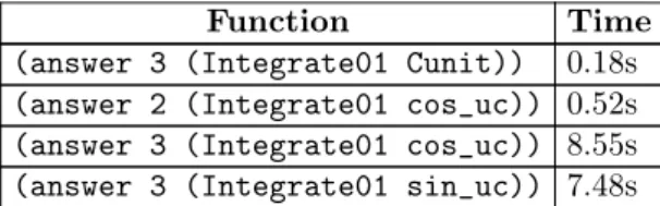
![Figure 12.1. Given two step functions f and g, the step function f ⊲ o ⊳ g is f squeezed into [0,o] and g squeezed into [o,1].](https://thumb-us.123doks.com/thumbv2/123dok_us/1898289.2777538/116.722.197.526.594.890/figure-given-step-functions-step-function-squeezed-squeezed.webp)

![Figure 13.1. A theorem in Coq stating that a plot on a 42 by 18 raster is close to the graph of the exponential function on [−6, 1].](https://thumb-us.123doks.com/thumbv2/123dok_us/1898289.2777538/142.722.119.610.79.430/figure-theorem-stating-raster-close-graph-exponential-function.webp)