Real Business Cycles in Emerging Countries?

NBER WORKING PAPER SERIES

REAL BUSINESS CYCLES IN EMERGING COUNTRIES? Javier García-Cicco

Roberto Pancrazi Martín Uribe Working Paper 12629

http://www.nber.org/papers/w12629

NATIONAL BUREAU OF ECONOMIC RESEARCH 1050 Massachusetts Avenue

Cambridge, MA 02138 October 2006

We thank for comments Stephanie Schmitt-Grohé, Vivian Yue, Viktor Todorov, Andy Neumeyer, Alejandro Gay, and seminar participants at the Federal Reserve Bank of San Francisco, the International Monetary Fund, HEC Montreal, Universidad de San Andrés (Buenos Aires), and the XI Workshop in International Economics and Finance held at Universidad Torcuato Di Tella. The views and conclusions presented in this paper are exclusively those of the authors and do not necessarily reflect the position of the Central Bank of Chile, its Board members, or the National Bureau of Economic Research. © 2006 by Javier García-Cicco, Roberto Pancrazi, and Martín Uribe. All rights reserved. Short sections of text, not to exceed two paragraphs, may be quoted without explicit permission provided that full credit, including © notice, is given to the source.

Real Business Cycles in Emerging Countries?

Javier García-Cicco, Roberto Pancrazi, and Martín Uribe NBER Working Paper No. 12629

October 2006, Revised December 2009 JEL No. F41

ABSTRACT

We use more than one century of Argentine and Mexican data to estimate the structural parameters of a small-open-economy real-business-cycle model driven by nonstationary productivity shocks. We find that the RBC model does a poor job at explaining business cycles in emerging countries. We then estimate an augmented model that incorporates shocks to the country premium and financial frictions. We find that the estimated financial-friction model provides a remarkably good account of business cycles in emerging markets and, importantly, assigns a negligible role to nonstationary productivity shocks.

Javier García-Cicco Duke University

Department of Economics 213 Social Science Building Box 90097 Durham, NC 27708 [email protected] Roberto Pancrazi Department of Economics Duke University Durham, NC 27708 [email protected] Martín Uribe Department of Economics Columbia University

International Affairs Building New York, NY 10027

and NBER

1

Introduction

Recently, a number of studies have departed from the mainstream view that in order to explain economic fluctuations in emerging markets theoretical models must take explicitly into account the role of policy and market failures. This line of research argues that business cycles in emerging countries can be explained well using a neoclassical model featuring no distortions and driven solely by shocks to total factor productivity. Finn Kydland and Carlos Zarazaga (2002), for instance, adopt a strong view by arguing that the RBC model can replicate satisfactorily the ‘lost decade’ of the 1980s in Argentina. More recently Mark Aguiar and Gita Gopinath (2007) have suggested that an RBC model driven primarily by permanent shocks to productivity can explain well business cycles in developing countries. These authors acknowledge the fact that shocks impinging upon emerging countries are numerous and of different natures, but argue that their combined effect can be modeled as an aggregate shock to total factor productivity with a large nonstationary component. In addition, they argue that the neoclassical model is an adequate framework for understanding the transmission of such shocks.

In this paper, we undertake an investigation of the hypothesis that an RBC model driven by a combination of permanent and transitory shocks to total factor productivity can account satisfactorily for observed aggregate dynamics in developing countries. To this end, we conduct an econometric estimation of the parameters of a small open economy RBC model using Argentine and Mexican data over the period 1900-2005. Our use of long time series is motivated by what we believe is an important drawback of existing studies advocating the ability of the RBC model driven by permanent technology shocks to explain business cycles in developing countries. Namely, the use of short samples both for the characterization of observed business cycles and for the estimation of the parameters of the theoretical model, particularly those defining the stochastic process of the nonstationary productivity shock.

We find that, when estimated over the long sample, the RBC model driven by perma-nent and transitory productivity shocks does a poor job at explaining observed business cycles in Argentina and Mexico along a number of dimensions. One such dimension is the trade-to-output ratio. Specifically, the RBC model predicts that the trade balance-to-output ratio is a near random walk, with a flat autocorrelation function close to unity. By contrast, in the data, the highest autocorrelation coefficient of the trade balance-to-output ratio takes place at the first order and is less than 0.6, with higher-order autocorrelations converging quickly to zero. In addition, we find that the RBC model fails to match several other important features of the business cycle in emerging countries. In particular, in Ar-gentina and Mexico, as well as in many other emerging countries, consumption is significantly

more volatile than output. The RBC model fails to capture the observed excess volatility in consumption, and in the case of Mexico it actually predicts consumption to be significantly less volatile than output. Also, the model predicts the trade balance to be significantly more volatile than its corresponding empirical counterpart. Furthermore, the RBC model does poorly at matching the correlation of the trade balance with the domestic components of aggregate absorption.

To gauge the role of nonstationary productivity shocks in explaining business cycles in emerging countries, we estimate using Bayesian methods an augmented version of the baseline RBC model that incorporates preference shocks, country-premium shocks and a realistic debt elasticity of the country premium. The latter two features are meant to capture in a simplified form an economy facing international financial frictions. We find that the augmented model mimics remarkably well the observed business cycles in Argentina over the period 1900-2005. In particular, the model replicates the downward-sloping autocorrelation function of the trade-balance-to-output ratio, the excess volatility of consumption, the high volatility of investment, and a volatility of the trade-balance-to-output ratio comparable to that of output growth. Importantly, the estimated model assigns a negligible role to permanent productivity shocks lending little support to the hypothesis that the cycle is the trend.

The remainder of the paper is organized as follows: Section 2 analyzes empirical regulari-ties of business cycles in emerging countries. It argues that, contrary to the moderation that took place in developed countries after the second world war, the amplitude and frequency of business cycles in emerging countries has been stable over the past century. Section 3 presents the RBC model. Section 4 describes the econometric estimation of the model using Bayesian methods and Argentine data from 1900 to 2005. It also evaluates the per-formance of the RBC model. Section 5 develops, estimates, and evaluates a version of the model that incorporates financial frictions, country spread shocks, preference shocks, and domestic-spending shocks. Section 6 estimates the model using Mexican data over the pe-riod 1900-2005 and relates the results to those obtained in the related literature that uses shorter samples. Section 7 concludes.

2

Business Cycles in Emerging Countries: 1900-2005

Our joint analysis of pre- and post-world-war-two data represents a departure from the usual practice in studies of the developed-country business cycle. Typically, these studies concentrate either on the pre-world-war-two period—often emphasizing the Great Depression years—or on the post-world-war-two period—as do most of the many papers spurred by the

work of Finn Kydland and Edward Prescott (1982). There is a good reason for separating the pre- and post-world-war-two periods when examining developed-country data. For the volatility of business cycles in industrialized countries fell significantly in the second half of the twentieth century. In sharp contrast, in emerging countries business cycles do not appear to moderate after the second world war. This fact is clearly illustrated in figure 1, which depicts the evolution of output in Argentina (panel a) and the United States (panel b) over the period 1900-2005. Data sources are presented in the appendix. The figure shows with solid lines the logarithm of GDP per capita and with broken lines the associated cubic trend. In the United States, the first half of the twentieth century is dominated by the Great Depression and appears as highly volatile. By comparison, the half century following the end of World War II appears as fairly calm, with output evolving smoothly around its long-run trend. On the other hand, in Argentina output fluctuations appear equally volatile in the prewar period as in the postwar period.1 _{More specifically, over the period 1900-2005 the}

United States and Argentina display similar volatilities in per-capita output growth of about 5 percent. However, in the United States the volatility of output growth falls significantly from 6.4 percent in the prewar period to 3.4 percent in the postwar period. By contrast, in Argentina the volatility of output growth falls insignificantly from 5.7 in the earlier half of the twentieth century to 5.2 percent in the later half.

The patterns of aggregate volatility observed in Argentina and the United States extend to larger sets of developed and emerging countries. Figure 2 displays the cyclical component of the log of real GDP per capita for seven Latin American countries and thirteen small developed countries over the period 1900-2005. In the figure, the cycle is computed as percent deviations of GDP from a cubic trend. Three main conclusions emerge from the data presented in figure 2. First, over the period 1900-2005, business cycles are equally volatile in the group of Latin American countries as in the group of developed countries. The average standard deviation of detrended output is about 10 percent for both groups. Second, in the group of Latin American economies, business cycles are as volatile in the period 1900-1945 as in the period 1946-2005, with average standard deviations of 10.1 and 9.8 percent, respectively. By contrast, in the group of developed countries business cycles are significantly more volatile in the period 1900-1945 than in the period 1946-2005, with average standard deviations of 12.7 percent versus 7.2 percent, respectively. Third, the period

1980-1_{Susanto Basu and Alan M. Taylor (1999) also find no differences in output volatility in Argentina in}

the prewar and postwar eras (see their table A3). Using data from Argentina for the period 1884 to 1990, Adolfo Sturzenegger and Ramiro Moya (2003) find that business cycles in the pre world war II period were more volatile than in the postwar period. This different result is due to the fact that their sample does not include the years 1991-2005, which are among the most volatile of the postwar era and that their sample includes the period 1884-1900, which was particularly volatile (see Basu and Taylor, 1999, table A3).

(a) Argentina 19000 1910 1920 1930 1940 1950 1960 1970 1980 1990 2000 0.2 0.4 0.6 0.8 1 year Log gdp per capita

Cubic trend (b) United States 19000 1910 1920 1930 1940 1950 1960 1970 1980 1990 2000 0.2 0.4 0.6 0.8 1 1.2 1.4 1.6 1.8 2 year Log gdp per capita

Cubic trend

(a) Latin America 1900 1910 1920 1930 1940 1950 1960 1970 1980 1990 2000 −0.8 −0.7 −0.6 −0.5 −0.4 −0.3 −0.2 −0.1 0 0.1 0.2 0.3 Argentina Brazil Chile Colombia Mexico Peru Uruguay Venezuela

(b) Small Developed Economies

1900 1910 1920 1930 1940 1950 1960 1970 1980 1990 2000 −0.8 −0.7 −0.6 −0.5 −0.4 −0.3 −0.2 −0.1 0 0.1 0.2 0.3 Australia Austria Belgium Canada Denmark Finland Iceland Netherlands New Zealand Norway Portugal Spain Sweden Switzerland

Figure 2: Business Cycles in Small Economies: 1900-2005

Note. Percent deviations of real GDP per capita from a cubic trend.

Source: Data base compiled by R. Barro and J. Urs´ua, available on line at http://www.economics.harvard.edu/faculty/barro/data sets barro.

2005 contains only between one and a half and two cycles for most of the Latin American economies included in the figure. This fact suggests that if one is to uncover the importance of permanent productivity shocks as drivers of business cycles in emerging countries , limiting the empirical analysis to the post 1980 period—as do many recent related studies—may be problematic. The empirical evidence presented thus far serves as motivation for our focus on a long sample for the analysis of business cycles in emerging countries.

2.1

The Autocorrelation Function of the Trade-Balance-To-Output

Ratio

At center stage in virtually every study of the business cycle in emerging economies is the trade balance. Examples of strands of the literature in which this variable features prominently include the literatures on balance of payments crises, sudden stops, sovereign debt, and exchange-rate-based stabilization. One reason for the interest in understanding the behavior of this variable is that typically the onset of economic crises in emerging countries are characterized by large reversals in the trade balance. It is therefore natural to ask whether the RBC model can capture observed movements of the trade balance over the business cycle. More specifically, one of the dimensions along which we will scrutinize the empirical performance of the RBC model is the autocorrelation function of the trade-balance-to-output ratio.

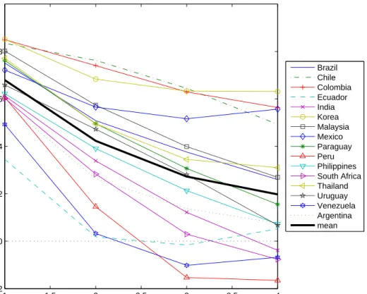
Figure 3 displays the autocorrelation function of the trade-balance-to-output ratio of sixteen emerging countries. Although there is some variation across countries, the pattern that emerges is that of a downward-sloping function with a first-order autocorrelation of about 0.65 and that approaches zero monotonically at the fourth or fifth order.

2.2

Second Moments: Argentina 1900-2005

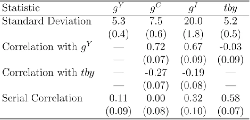
Table 1 displays empirical second moments of output growth, consumption growth, invest-ment growth, and the trade-balance-to-output ratio for Argentina over the period 1900-2005. Argentina is one of two countries for which we constructed long time series for the four vari-ables considered in the table. The other country is Mexico, which we analyze in section 6.

Notably, unlike in developed countries, per-capita consumption growth in Argentina is significantly more volatile than per-capita output growth. The excess volatility of consump-tion relative to output is more than two percentage points. Others have documented this fact for Argentina and other emerging countries using post-1980 data (Pablo A. Neumeyer and Fabrizio Perri, 2006, Aguiar and Gopinath, 2007, and Mart´ın Uribe, 2006). Here, we show that the high volatility of consumption relative to output remains present after augmenting

1 1.5 2 2.5 3 3.5 4 −0.2 0 0.2 0.4 0.6 0.8 order Emerging Countries Brazil Chile Colombia Ecuador India Korea Malaysia Mexico Paraguay Peru Philippines South Africa Thailand Uruguay Venezuela Argentina mean

Figure 3: The Autocorrelation Function of the Trade Balance-to-Output Ratio in Emerging Countries

Note: The data are annual. The samples are: Argentina, 1900-2005; Brazil, 1947-2007; Chile, 1967-1947-2007; Colombia, 1925-1947-2007; Ecuador, 1950-2006; India, 1950-1947-2007; South Korea, 2006; Malaysia, 1955-2007,; Mexico, 1900-2005; Paraguay, 1953-2008; Peru, 1950-2007; Philippines, 1948-2007; South Africa, 1950-2006; Thailand, 1950-2007; Uruguay, 1955-2007; and Venezuela, 1950-2007. The source is IFS, except for Brazil (IBGE), Colombia (Departamento Nacional de Planeacion), and Argentina and Mexico (see the appendix).

Table 1: Second Moments: Argentina 1900-2005 Statistic gY _gC _gI _tby Standard Deviation 5.3 7.5 20.0 5.2 (0.4) (0.6) (1.8) (0.5) Correlation withgY _{— 0.72 0.67 -0.03} — (0.07) (0.09) (0.09)

Correlation withtby — -0.27 -0.19 —

— (0.07) (0.08) —

Serial Correlation 0.11 0.00 0.32 0.58

(0.09) (0.08) (0.10) (0.07)

Note: gY, gC, andgI denote the growth rates of output per capita, consumption per capita, and investment per capita, respectively, and tby denotes the trade balance-to-output ratio. Standard deviations are reported in percentage points. Standard errors are shown in parenthesis. The data is annual, and the sources are given in the appendix.

the sample to include the first three quarters of the twentieth century. Gross investment growth is enormously volatile. Its standard deviation is about four times as large as that of output growth. At the same time, the trade balance-to-output ratio is about as volatile as output growth. The observed correlation between the trade balance-to-output ratio and output growth is negative but insignificantly different from zero. By contrast the domestic components of aggregate demand, private consumption growth and investment growth, are significantly negatively correlated with the trade balance. Finally, the bottom row of table 1 shows that the first-order autocorrelation of output growth is positive but small and not significantly different from zero.

3

The RBC Model

The theoretical framework is the small open economy model presented in Stephanie Schmitt-Groh´e and Uribe (2003) augmented with permanent productivity shocks as in Aguiar and Gopinath (2007). The production technology takes the form

Yt =atKtα(Xtht)1−α, (1)

whereYtdenotes output in periodt,Ktdenotes capital in periodt,htdenotes hours worked in

periodt, andat andXtrepresent productivity shocks. Our interpretation of these two sources

disturbances that may affect total factor productivity, such as terms-of-trade shocks. We use upper case letters to denote variables that contain a trend in equilibrium, and lower case letters to denote variables that do not contain a trend in equilibrium.

The productivity shock at is assumed to follow a first-order autoregressive process in logs.

That is, lnat+1 =ρalnat +at+1; a t ∼N(0, σ 2 a).

The productivity shock Xt is nonstationary. Let

gt ≡

Xt

Xt−1

denote the gross growth rate ofXt. We assume that the logarithm of gt follows a first-order

autoregressive process of the form

ln(gt+1/g) =ρgln(gt/g) + g t+1; g t ∼N(0, σ 2 g).

The parameter g measures the deterministic gross growth rate of the productivity factorXt.

The parameters ρa, ρg ∈[0,1) govern the persistence of at and gt, respectively.

Household face the following period-by-period budget constraint:

Dt+1 1 +rt =Dt−Yt+Ct+It + φ 2 Kt+1 Kt −g 2 Kt, (2)

where Dt+1 denotes the stock of debt acquired in period t, rt denotes the domestic interest

rate on bonds held between periods t and t+ 1, Ct denotes consumption, It denotes gross

investment, and the parameterφ introduces quadratic capital adjustment costs. The capital stock evolves according to the following law of motion:

Kt+1 = (1−δ)Kt+It, (3)

where δ∈[0,1) denotes the depreciation rate of capital.

In order to induce independence of the deterministic steady state from initial conditions, we assume that the country faces a debt-elastic interest-rate premium as in Schmitt-Groh´e and Uribe (2003). Specifically, the domestic interest rate is assumed to be the sum of the world interest rater∗ _{>0, assumed to be constant, and a country premium that is increasing}

in a detrended measure of aggregate debt as follows:

rt =r∗+ψ

eDet+1/Xt−d¯_−1,

Table 2: Calibration

Parameter γ δ α ψ ω θ β d¯

Value 2 0.1255 0.32 0.001 1.6 2.24 0.9224 0.007

The variable ˜Dt denotes the aggregate level of external debt per capita, which the household

takes as exogenous. In equilibrium, we have that ˜Dt =Dt.

Consumers are subject to a no-Ponzi-scheme constraint of the form limj→∞Et

Dt+j

Qj

s=0(1+rs)

≤

0. The household seeks to maximize the utility function

E0 ∞ X t=0 βt[Ct−θω −1 Xt−1hωt] 1−γ −1 1−γ , (4)

subject to (1)- (3) and the no-Ponzi-game constraint, taking as given the processes at, Xt,

and rt and the initial conditions K0 and D−1. The household’s optimality conditions and

the complete set of equilibrium conditions in stationary form are presented in Garc´ıa-Cicco, Pancrazi, and Uribe (2009).

4

Estimation and Evaluation of the RBC Model:

Ar-gentina 1900-2005

The time unit in the model is meant to be a year. We assign values to the structural parameters using a combination of calibration and econometric estimation techniques.

We calibrate the parameters α, δ, ψ, ¯d, θ, ω, and γ using long-run data relations from Argentina as well as parameter values that are common in related business-cycle studies. Table 2 presents the calibrated parameter values. We set the parameter ¯d to induce a small steady-state trade balance-to-output ratio of about 0.25 percent, as observed on average in Argentina over the period 1900-2005. We follow Schmitt-Groh´e and Uribe (2003) and assign a small value to the parameter ψ, measuring the sensitivity of the country interest-rate premium to deviations of external debt from trend, with the sole purpose of ensuring independence of the deterministic steady state from initial conditions, without affecting the short-run dynamics of the model. The value assigned to the depreciation rate δ implies an average investment ratio of about 19 percent, which is in line with the average value observed in Argentina between 1900 and 2005. The value assumed for the discount factor

β implies a relatively high average real interest rate of about 8.5 percent per annum, which is empirically plausible for an emerging market like Argentina. There is no reliable data on

factor income shares for Argentina. We therefore set the parameter α, which determines the average capital income share, at 0.32, a value commonly used in the related literature. We set θ = 2.24, to ensure that in the steady state households allocate about 20 percent of their time to market work. The parameter γ, defining the curvature of the period utility function, takes the value 2, which is standard in related business-cycle studies. Finally, ω

is calibrated at 1.6, which implies a labor-supply elasticity of 1/(ω−1) = 1.7. This value is frequently used in calibrated versions of small open economy models (see Mendoza, 1991; and Schmitt-Groh´e and Uribe, 2003).

We estimate the remaining parameters of the model using Bayesian methods and Ar-gentine data on output growth, consumption growth, investment growth, and the trade-balance-to-output ratio over the period 1900-2005. Specifically, we estimate six structural parameters, namely, the five parameters defining the stochastic process of the productivity shocks, g, σg, ρg, σa, and ρa and the parameter governing the degree of capital adjustment

costs, φ. We also estimate four nonstructural parameters representing the standard devia-tions of i.i.d. measurement errors on the observables, σy,σc,σi, andσtby. We impose uniform

prior distributions on all estimated parameters. Measurement errors are permitted to absorb no more than 6 percent of the variance of the corresponding observable time series. Table 3 presents key statistics of the prior and posterior distributions. The reported posterior sta-tistics are computed from a two-million MCMC chain from which the first one million draws were discarded. The estimation delivers quite persistent processes for both productivity shocks (i.e., high values of ρg and ρa) and a relatively large value for the adjustment-cost

parameter φ.

4.1

The Performance of the RBC Model

Figure 4 displays with a circled line the autocorrelation functions of the trade balance-to-output ratio implied by the RBC model. To facilitate comparison with the data, the figure reproduces with a solid line the corresponding estimated autocorrelation function, and with broken lines a two-standard-deviation confidence interval around the point estimate. All four autocorrelations predicted by the RBC model take values close to unity, indicating that in the model the trade balance-to-output ratio behaves as a near random walk. By contrast, the empirical autocorrelation function takes a value slightly below 0.6 at order one and then declines quickly toward zero, resembling a variable with a stationary autoregressive behavior. Further, the theoretical autocorrelation function lies entirely outside the two-standard-deviation band around the empirical point estimate.

The result that the autocorrelation function of the trade balance to output ratio

Table 3: Prior and Posterior Distributions

Posterior Distribution

Prior Distribution Financial-Frictions Model RBC Model

Parameter Min Max Median 5% 95% Median 5% 95 %

g 1 1.03 1.01 1.003 1.017 1.005 1.001 1.012 σg 0 0.2 0.0071 0.00057 0.027 0.03 0.019 0.042 ρg -0.99 0.99 0.35 -0.66 0.83 0.828 0.743 0.919 σa 0 0.2 0.033 0.028 0.038 0.027 0.024 0.032 ρa -0.99 0.99 0.87 0.79 0.93 0.765 0.621 0.888 φ 0 8 4.6 3 6.5 3.3 2.3 4.9 σν 0 1 0.51 0.37 0.8 ρν -0.99 0.99 0.86 0.74 0.93 σs 0 0.2 0.015 0.0014 0.05 ρs -0.99 0.99 0.29 -0.73 0.92 σµ 0 0.2 0.056 0.034 0.08 ρν -0.99 0.99 0.91 0.83 0.97 ψ 0 5 2.8 1.3 4.6 Measurement Errors σyme 0.0001 0.013 0.00011 0.0001 0.00014 0.0001 0.0001 0.0003 σcme 0.0001 0.019 0.00012 0.0001 0.00019 0.0011 0.0008 0.0014 σme i 0.0001 0.051 0.0012 0.00024 0.0032 0.0216 0.0169 0.0281 σ_tbyme 0.0001 0.013 0.00011 0.0001 0.00013 0.0001 0.0001 0.0002 Log-Marginal Likelihood 600.5854 547.5925

Note: Estimation is based on Argentine data from 1900 to 2005. All prior distributions are uniform. Posterior statistics are based on a two-million MCMC chain from which the first million draws were discarded. The upper bound of the prior distributions of the standard deviations of measurement errors equal 25 percent of the standard deviation of the corresponding empirical time series. The log-marginal likelihood was computed using Geweke’s modified harmonic mean method with truncation parameter 0.1. Differences of log-marginal likelihood across models are stable for different values of the truncation parameter.

Figure 4: The Predicted Autocorrelation Function of the Trade Balance-to-Output Ratio 1 1.5 2 2.5 3 3.5 4 −0.4 −0.2 0 0.2 0.4 0.6 0.8 1 lags RBC Model Financial−Friction Model Data Data ± 2std

dicted by the RBC model is flat and close to unity is not a consequence of the presence of nonstationary productivity shocks. Specifically, shutting off the nonstationary productivity

shock in the RBC model by setting σg equal to zero and keeping all other parameter

val-ues unchanged results in an autocorrelation function that is virtually identical to the one shown with a circled line in figure 4. Given our parameterization of the RBC model, the flat nature of the trade-balance-to-output ratio reflects the endogenous random walk of con-sumption typical of small open economies with incomplete asset markets. Our RBC model does not generate an exact endogenous random walk in consumption because we

incorpo-rate a small debt elasticity of the country interest incorpo-rate (governed by the parameter ψ) that

induces stationarity. However, because the debt-elasticity of the country premium is small, consumption is highly persistent in equilibrium. In general, however, the value assigned to

the parameter ψ is not the only determinant of the shape of the autocorrelation function of

the trade-balance-to-output ratio in the small open economy RBC model. In effect, given the

value ofψ, the values assigned to other parameters (such as the degree of capital adjustment

costs or the persistence of the stationary productivity shock, among others) can deliver a low and downward sloping autocorrelation function of the trade-balance-to-output ratio. This is

the case, for instance in the RBC model analyzed by Schmitt-Groh´e and Uribe (2003). The

Schmitt-Groh´e and Uribe model is of particular interest for the present discussion because it

features the same value of ψ as the one used in our parameterization of the RBC model, but

different values for other structural parameters. However, an autocorrelation of the trade-balance-to-output ratio that is flat and close to unity is a robust prediction of the small open economy RBC model in the following sense: Given the values of all other structural parameters of the model, there exists a small enough value of the parameter ψ, governing the debt-sensitivity of the country premium, that, up to first order, ensures stationarity of the equilibrium dynamics and at the same time delivers an autocorrelation function of the trade-balance-to-output ratio that is flat and close to unity.

One way to eliminate the near random walk behavior of the trade balance is to intro-duce financial imperfections as in the sovereign debt literature. In such environments trade deficits that result in increases in the net foreign debt position cause increases in the country premium, because, for instance, of elevated risks of default. In turn, larger country premia tend to incentivate domestic savings and discourage private investment, thereby dampening the increase in trade deficits. An ad-hoc way of capturing this channel in the context of the present model would be to sufficiently raise the value of the parameter ψ governing the debt-elasticity of the country premium. By placing financial frictions at center stage, how-ever, this type of transmission mechanism would represent a significant departure from the RBC paradigm. We explore the empirical relevance of financial frictions in section 5. Alter-natively, a downward-sloping autocorrelation function of the trade-balance-to-output ratio could be obtained by adopting a sufficiently elastic subjective discount factor with respect to consumption or a sufficiently large cost of adjusting the net foreign asset position. Again, assigning to any of these avenues a role larger than that of merely inducing stationarity, would imply a departure from the RBC paradigm.

Table 4 reports second moments implied by the RBC model. To facilitate comparison, the table reproduces the empirical counterparts and their associated standard errors from table 1. In the RBC model, consumption growth is slightly more volatile than output growth. This prediction is qualitatively in line with the data, but falls short quantitatively, as the RBC model predicts the excess volatility of consumption to be about half a percentage point, whereas in the data it is more than two percentage points. The insufficient excess volatility of consumption comes about not because consumption is predicted to be too smooth, but because output is predicted to be too volatile. In effect, the RBC model overestimates the volatility of output growth by about 2 percentage points. More importantly, the modest excess volatility of consumption predicted by the RBC model comes at the cost of an enor-mous implied volatility of the trade balance to output ratio of about twenty times the value observed in the data.

To a large extent, both the excess volatility of consumption relative to output and the volatility of the trade-balance-to-output ratio are the consequence of a high estimated value

Table 4: Comparing Model and Data: Second Moments Statistic gY gC gI tby Standard Deviation – RBC Model 7.2 7.6 12.9 106.6 – Financial-Frictions Model 6.3 8.4 17.7 5.1 – Data 5.3 7.5 20.4 5.2 (0.4) (0.6) (1.8) (0.6) Correlation withgY – RBC Model 0.88 0.77 -0.02 – Financial-Frictions Model 0.79 0.35 -0.02 – Data 0.72 0.67 -0.04 (0.07) (0.09) (0.09) Correlation withtby

– RBC Model -0.02 -0.03 – Financial-Frictions Model -0.28 -0.24 – Data -0.27 -0.19 (0.07) (0.08) Serial Correlation – RBC Model 0.28 0.13 0.06 0.99 – Financial-Frictions Model 0.04 -0.01 -0.09 0.53 – Data 0.11 -0.01 0.32 0.58 (0.09) (0.08) (0.10) (0.07)

Note: Empirical moments are computed using Argentine data from 1900 to 2005. Standard deviations are reported in percentage points. Standard errors of sample-moment estimates are shown in parenthesis. Model sample-moments are computed as the median based on 400,000 draws from the posterior distribution.

for the parameter ρg, measuring the persistence of the growth rate of the nonstationary

component of total factor productivity, Xt/Xt−1. In effect, if one lowers the value of ρg

from its posterior median level of 0.82 to 0 holding all other parameter values equal (so that the growth rate of the nonstationary component of productivity becomes both less persistent and unconditionally less volatile), consumption becomes significantly less volatile than output and the trade-balance-to-output ratio becomes about eighty percentage points less volatile (although still several times more volatile than in the data). The intuition behind this result is as follows. When the growth rate of the nonstationary component of productivity is highly persistent, a positive permanent innovation in productivity (gt > 0)

generates positive growth rates in productivity not only in the current period but also in the future. As a consequence, the trend level of productivity becomes steeper. Faced with this upward-sloping revision in the path of productivity, agents decide to smooth consumption by borrowing against future income. Thus, current consumption increases beyond current output and the trade balance deteriorates. So the volatilities of consumption growth and the trade balance move hand in hand with changes in the persistence of productivity growth. This is problematic because although a reduction in ρg improves the performance of the

RBC model by making the trade balance less volatile, it worsens its performance by making consumption less volatile relative to output.

The intuition provided in the previous paragraph suggests that another parameter that may play a significant role in determining both the excess volatility of consumption and the volatility of the trade balance is σg, the standard deviation of the innovation in the growth

rate of the nonstationary component of productivity. This is indeed the case. Shutting off the nonstationary productivity shock by setting σg equal to zero lowers the volatility of

the trade-balance-to-output ratio to about 25 percent but it also results in a volatility of consumption growth significantly lower than that of output growth. As in the case of ρg,

lowering σg improves the performance of the RBC model along one dimension (the volatility

of the trade balance) but in detriment of another important dimension (the excess volatility of consumption relative to output).

The RBC model significantly underpredicts the volatility of gross investment (12.9 in the model versus 20.4 percent in the data). A higher volatility of the nonstationary productivity shock would contribute to narrowing this difference, but at the expense of exacerbating the immense overestimation of the volatility of the trade-balance-to-output ratio.

Finally, the RBC model correctly predicts a near-zero correlation between output growth and the trade balance-to-output ratio. However, it significantly underpredicts the negative correlations of the trade-balance-to-output ratio with consumption growth and investment growth. The fact that the trade-balance share is more correlated with the domestic

com-ponents of aggregate demand than with output growth may be an indication that shocks other than movements in total factor productivity could be playing a role in driving business cycles in Argentina. We explore this possibility next..

5

Financial Frictions and Country-Spread Shocks

The goal of this section is to build and estimate a model in which the sources of uncertainty and the transmission mechanism invoked by the RBC model compete with additional shocks and frictions. To this end, we augment the RBC model with a simple form of financial friction, and with shocks to the country premium and to domestic absorption. Specifically, we now allow the parameter ψ, governing the debt elasticity of the country premium, to be econometrically estimated, rather than fixing it at a small number. In this way, the role of the debt elasticity of the country premium is no longer limited to simply inducing stationarity, but to potentially act as the reduced form of a financial friction shaping the model’s response to aggregate disturbances. The additional sources of uncertainty include a domestic preference shock, a spending shock, which may be interpreted as a government purchases shock, and a country premium shock. We interpret the shock to the country premium as possibly stemming from financial imperfections that open the door to stochastic shifts in the country premium that are uncorrelated with the state of domestic fundamentals. Uribe and Vivian Yue (2006) find that this type of disturbance explain about two thirds of movements in country premia in emerging countries. To distinguish it from the standard RBC model studied thus far, we will refer to the model presented in this section as a ‘model with financial frictions.’

Formally, in the augmented model households seek to maximize

E0 ∞ X t=0 νtβt [Ct−θω−1Xt−1hωt] 1−γ −1 1−γ ,

subject to the sequential resource constraint

Dt+1 1 +rt =Dt−Yt+Ct+St +It + φ 2 Kt+1 Kt −g 2 Kt,

and to the no-Ponzi-game condition given above. The variablesνt and St represent,

respec-tively, an exogenous and stochastic preference shock and a domestic spending shock following the AR(1) processes

lnνt+1 =ρνlnνt +νt+1; ν t ∼i.i.d. N(0, σ 2 ν). 17

and ln(st+1/s) =ρsln(st/s) +st+1; s t ∼i.i.d. N(0, σ 2 s),

where st ≡St/Xt−1. The country premium takes the form

rt =r∗+ψ

eDet+1/Xt−d¯₋₁

+eµt−1_−1,

where µt represents an exogenous stochastic country premium shock following the AR(1)

process lnµt+1 =ρµlnµt+ µ t+1; µ t ∼i.i.d. N(0, σ 2 µ).

All other elements of the model, including the production technology, the evolution of the stationary and nonstationary productivity shocks, and the evolution of the capital stock are as in the baseline RBC model presented above. Note that the present model nests the baseline RBC model of section 3.

We estimate the model using Bayesian methods and Argentine data on output growth, consumption growth, investment growth, and the trade-balance-to-output ratio over the period 1900-2005. We estimate 13 structural parameters, σg, ρg, σa, ρa, σν, ρν, σs, ρs,

σµ, ρµ, φ, ψ, and g, and 4 nonstructural parameters representing the standard deviations

of i.i.d. measurement errors on the observables, σy, σc, σi, and σtby. We impose uniform

prior distributions on all estimated parameters. Table 3 shows key statistics of the prior and posterior distributions. We highlight the following features: First, the posterior distributions of the parametersσg andρg defining the nonstationary productivity shock are quite disperse,

with 90-percent probability intervals of (0.0006,0.03) and (−0.66,0.83), respectively. This result suggest a weak identification of the trend shock to productivity. Second, the median of

σg takes the value 0.007, which is four times smaller than the corresponding point estimate

in the baseline RBC model, suggesting a reduced importance of the permanent technology shock under the present specification. Third, the estimated distribution of the parameter

ψ implies a high sensitivity of the country premium to the level of external debt. The posterior median of this parameter is estimated to be 2.8, which implies that if the stock of external debt increases by one percentage point of GDP then the country premium increases by over half a percentage point. This finding indicates that the data assign a nonnegligible role to financial frictions. Fourth, the estimated volatility of the country-premium shock is large. The median value of σµ of 0.056 implies that a one-standard-deviation innovation

in µt raises the interest rate at which the country borrows from world financial markets by

about 5 percentage points. The bottom panel of table 3 presents the log-marginal likelihoods associated with the RBC and financial-friction models. These statistics indicates that the

data favor the financial-friction model over the RBC specification.

Figure 4 displays with a crossed line the autocorrelation function of the trade-balance-to-output ratio predicted by the model. In producing this autocorrelation function, the structural parameters are set at the median of their posterior distributions. The figure shows that the model augmented with financial frictions is highly successful at replicating the downward-sloping autocorrelation function of the trade-balance-to-output ratio observed in Argentina over the period 1900-2005. This success is due to three features of the model. One is the financial friction captured by the parameter ψ, governing the sensitivity of the country premium to movements in the stock of external debt. When ψ is relatively high, deviations of the trade-balance ratio below its long-run level cause the external debt to increase, which, by the presence of a debt-elastic interest-rate premium, produces a rise in the country interest rate. In turn, elevated interest rates tend to curb the growth rates of consumption and investment, thereby inducing the trade balance to revert to its long-run level. A similar intuition applies to deviations of the trade-balance ratio above its long-run level. It follows that the larger is ψ the more trend reverting is the trade-balance ratio, and therefore the more downward-sloping is its autocorrelation function. Indeed, lowering the value of ψ from its median value of 2.8 to the small value of 0.001 imposed in the calibration of the baseline RBC model causes the autocorrelation function of the trade-balance-to-output ratio to become flat and close to unity as in the RBC model. The other two elements of the model that are important in mimicking the observed autocorrelation function of the trade-balance-to-output ratio are country-premium shocks and preference shocks. Shutting down these two shocks by setting σµ = σν = 0, while keeping all other

parameter values at their posterior medians, causes the autocorrelation function of the trade-balance-to-output ratio to lie entirely above the upper limit of the two-standard-error band around the empirical point estimate. On the other hand, productivity shocks are not essential for the model’s ability to match the autocorrelation function of the trade-balance-to-output ratio. In effect, shutting off both productivity shocks by setting σg =σa = 0 one obtains a

predicted autocorrelation function of the trade-balance-to-output ratio that matches quite well its empirical counterpart.

Table 4 displays second moments predicted by the model with financial frictions. The table shows that the augmented model overcomes a number of difficulties faced by the RBC model. First, the model with financial frictions captures the fact that in Argentina over the period 1900-2005, as in most other developing countries, consumption growth is significantly more volatile than output growth. Specifically, in accordance with the data, the financial-friction model predicts that consumption is about 2 percentage points more volatile than output. By contrast, the RBC model predicts that the excess volatility of

consumption is less than half a percentage point. In the financial-friction model the bulk of the predicted excess volatility of consumption is explained not by nonstationary productivity shocks—as maintained by the hypothesis that ‘the cycle is the trend’—but by domestic preference shocks. This observation will become apparent shortly when we present predicted variance decompositions. Second, the model with financial frictions corrects the RBC model’s severe overestimation of the volatility of the trade-balance-to-output ratio as well as the underestimation of the volatility of investment growth. Finally, as in the data, the model with financial frictions predicts a significant negative correlation of the trade-balance ratio with consumption and investment growth. By contrast, the RBC model predicts virtually no correlation between the trade balance and the components of domestic absorption.

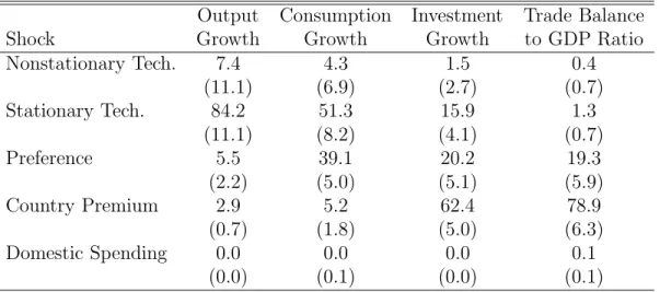
Table 5 presents the variance decomposition predicted by the model with financial

fric-Table 5: Variance Decomposition Predicted by the Model with Financial Frictions Output Consumption Investment Trade Balance

Shock Growth Growth Growth to GDP Ratio

Nonstationary Tech. 7.4 4.3 1.5 0.4 (11.1) (6.9) (2.7) (0.7) Stationary Tech. 84.2 51.3 15.9 1.3 (11.1) (8.2) (4.1) (0.7) Preference 5.5 39.1 20.2 19.3 (2.2) (5.0) (5.1) (5.9) Country Premium 2.9 5.2 62.4 78.9 (0.7) (1.8) (5.0) (6.3) Domestic Spending 0.0 0.0 0.0 0.1 (0.0) (0.1) (0.0) (0.1)

Note: Means based on 400,000 draws from the posterior distribution. Standard devi-ations are in parenthesis. The estimated contribution of all four measurement errors (not shown) is negligible for all four variables.

tions. The most remarkable result that emerges from this exercise is that the contribution of nonstationary productivity shocks to business cycles is predicted to be virtually nil. That is, the model gives little credence to the hypothesis that ‘the cycle is the trend.’ This result is in line with the findings of Javier Garc´ıa-Cicco (2008), in the context of a model with a richer set of shocks and frictions and using the same set of observables, and Roberto Chang and Andr´es Fernandez (2008), in a model with additional financial frictions and using Mexican data post 1980. By contrast, the stationary component of total factor productivity explains most of the predicted movements in output growth.

Disturbances in productivity, whether permanent or temporary, play virtually no role in explaining movements in investment growth or the trade balance-to-output ratio. These two variables are to a large extent driven by innovations in country interest rates. In addition, private consumption growth is explained in equal parts by domestic preference shocks and stationary productivity shocks. Importantly, preference shocks are responsible for most of the excess volatility of consumption growth over output growth. This result is in stark contrast with the hypothesis according to which the excess volatility of consumption observed in emerging countries is due to permanent movements in productivity. Finally, domestic spending shocks are estimated to have a negligible role in explaining business cycles.

6

Mexico 1900-2005

The case of Mexico is of interest because it has been used in earlier studies to test the potential of the RBC model driven by trend shocks to productivity to explain business cycles in emerging countries. We begin by estimating the RBC model using a long annual sample of Mexican data ranging from 1900 to 2005. We then compare the results with those obtained in related studies that use shorter samples for the estimation and the evaluation of the RBC model. To make the comparison with related studies a step closer, we estimate the model by GMM. Specifically, we estimate the parametersg,σg,ρg,σa,ρa, and φof the RBC

model using annual data on output growth, consumption growth, investment growth, and the trade-balance-to-output ratio from Mexico over the period 1900-2005 (see the appendix for data sources). In the GMM estimation, we include 16 moment conditions: the variances and first- and second-order autocorrelations of output growth (gY_{), consumption growth}

(gC_{), investment growth (g}I_{), and the trade balance-to-output ratio, (tby), the correlation}

of gY _{with g}C_{, g}I_{, and tby, and the unconditional mean ofg}Y_{. (See Garc´ıa-Cicco, Pancrazi,}

and Uribe, 2009, for more details.)

All calibrated parameters are set as in the Argentine case (table 2), except for d and

δ, which were set at 0.05 and 0.082, respectively, to match the Mexican average trade-balance-to-GDP ratio (1.25 percent) and average investment-to-GDP ratio (14.7) over the sample period. Table 6 displays point estimates and associated standard errors of the six structural parameters estimated by GMM. Table 7 displays empirical and theoretical second moments. The RBC model estimated using Mexican data counterfactually predicts that output is more volatile than consumption. In addition, the model overpredicts the volatilities of investment and the trade balance and underpredicts the volatility of consumption. The high volatility of investment growth predicted by the model is a consequence of the fact that the GMM estimate of the parameter φ governing the degree of capital adjustment costs is

Table 6: Mexico 1900-2005: Estimated Parameters Point Standard

Parameter Estimate Error

g 1.001 0.001 σg 0.017 0.003 ρg 0.247 0.096 σa 0.019 0.001 ρa -0.019 0.028 φ 0.000 0.002 Overidentifying

Restrictions Test pvalue 0.070

Table 7: Mexico 1900-2005 Statistic gY _gC _gI _tby Standard Deviation —Model 5.17 3.12 50.28 9.80 —Data 4.09 6.15 19.86 4.28 (0.64) (1.08) (2.91) (0.42) Correlation withgY —Model 0.98 0.08 -0.02 —Data 0.66 0.55 -0.20 (0.14) (0.08) (0.13) Correlation withtby

—Model -0.13 -0.44 —Data -0.29 -0.07 (0.07) (0.09) Serial Correlation —Model -0.38 -0.27 -0.55 0.62 —Data 0.09 -0.07 0.23 0.72 (0.10) (0.08) (0.13) (0.10)

Note: Standard deviations are reported in percentage points. Standard errors of sample-moment estimates are shown in parenthesis.

virtually zero. The model also overestimates the cyclicalities of consumption and the trade balance and overestimates the cyclicality of investment. Further, the RBC model severely underestimates the serial correlations of output, consumption, and investment. The model predicts a first-order autocorrelation of the trade-balance-to-output ratio significantly less than unity and close to its empirical counterpart. This result is due to the behavior of gross investment. The virtual absence of adjustment costs induces firms to bunch investment rather than spread this type of expenditure over time. As a result, investment growth is highly negatively serially correlated. In turn, the negative serial correlation of investment growth has a depressing effect on the first-order serial correlation of the trade balance. However, this effect represents only a parallel downward shift in the autocorrelation function of the trade balance, which is counterfactually flat. This point is conveyed graphically by figure 5, which shows that the autocorrelation function of the trade balance predicted by the Figure 5: Mexico 1900-2005: The Autocorrelation Function of the Trade Balance-to-Output Ratio 1 2 3 4 5 6 7 8 9 10 0.2 0.3 0.4 0.5 0.6 0.7 0.8 0.9 Model Data

model starts at around 0.6 but, is flat (indeed slightly increasing). To highlight the flatness of the predicted autocorrelation function of the trade-balance-to-output ratio, the figure displays autocorrelations up to order 10. However, the theoretical autocorrelation function remains above 0.6 way beyond order 100. By contrast, the empirical autocorrelation function is strictly decreasing and converges relatively quickly to zero.

We conclude that the RBC model with nonstationary productivity shocks does a poor

job at matching the Mexican business cycle over the period 1900-2005. This result is in stark contrast with the findings of Aguiar and Gopinath (2007) (henceforth AG), namely, that the RBC model driven by permanent shifts to productivity performs well over the shorter period 1980-2003. Why does the RBC model do a good job at matching the short-sample moments but a poor job at matching the long-sample moments? We begin to address this question by establishing that the different results are not due to the application of different econometric techniques in the AG paper and in the present study. This first step is in order because, unlike AG, and guided by our reading of the econometric literature on GMM estimation of business-cycle models with persistent time series, we HP filter neither the empirical nor the theoretical data before estimation. Instead, our estimation procedure uses growth rates of output, consumption, and investment and the trade-balance-to-output ratio. Accordingly, we estimate the RBC model employing the same data set used by AG (a quarterly sample of Mexican data covering the period 1980:Q1 to 2003:Q2), but applying the same GMM technique we used to estimate the model over the sample 1900-2005. We find that over the shorter sample the fit of the RBC model increases significantly. In particular, the model matches the volatilities of output, consumption, and the trade balance quite well. We note especially that the model predicts consumption to be as volatile as output. It overestimates the volatility of investment, but not significantly. Finally, the model estimated over a short sample does a good job at replicating the observed autocorrelation function of the trade-balance-to-output ratio up to the fourth order. (Details of this estimation exercise are available at Garc´ıa-Cicco, Pancrazi, and Uribe, 2009.) This result demonstrates that it is not differences in econometric techniques applied in the AG paper and in our paper that account for our finding that the RBC model performs significantly worse over the long sample.

A salient feature of the Mexican data that is to a large extent responsible for the better fit of the RBC model over the short sample than over the long sample is the higher volatility of consumption relative to output over the long sample. In effect, over the period 1900-2005, consumption growth was almost 50 percent more volatile than output growth, whereas over the shorter period 1980-2003 it was less than 25 percent more volatile than output growth. If appropriately parameterized, the RBC model driven by trend shocks to productivity can indeed generate high relative volatility of consumption. We showed earlier in the paper that this can be achieved by raising the persistence and/or the volatility of the nonstationary productivity shock. However, a byproduct of doing this is a higher implied volatility of the trade-balance-to-output ratio. This would not be a problem if the longer sample were characterized by a relatively more volatile trade-balance-to-output ratio than is the short sample. But this is not the case. On the contrary, over the period 1900-2005, the

trade-balance-to-output ratio was actually less volatile than output growth, whereas over the period 1980-2003 it was 15 percent more volatile than output growth.2 A natural question is therefore whether the long sample or the short sample is more suitable for characterizing business cycles in emerging countries. In section 2 of the paper, we show that for most Latin American economies the period 1980 to 2003 contains only one and a half to two business cycles, whereas the sample period 1900 to 2005 that we consider contains about nine business cycles. There, we also argue that the amplitude and frequency of business cycles in emerging countries has been stable over the past century. Taken together, these observations suggest that the long sample is more representative of business-cycle regularities in emerging countries than is the short sample.

One might argue that an advantage of using a relatively short sample is the possibility of picking a period of relative stability in macroeconomic policy. Arguably, a time span in which policy has been stable could be a more fertile ground for testing the explanatory power of an RBC model—in which, by design, government intervention is completely absent—than a period characterized by frequent policy regime switches. Stability is, however, hardly a characteristic of Mexican macroeconomic policy over the period 1980 to 2003. We briefly point out three policy areas along which Mexico experienced major swings over the period in question. One is financial regulation. The Mexican financial sector was relatively unreg-ulated until 1982 when, in response to the developing-country debt crisis, the government applied severe financial repression, which included the nationalization of the banking sector. Financial policy changed again in the mid 1980s, when these regulations were removed. A second source of policy heterogeneity during this period was monetary policy. High inflation during the period 1982-1987 was followed, as a result of an exchange-rate-based stabilization program, by a period of relative price stability over the period 1987-1994. The so called Tequila crisis rendered the antiinflationary policy unsustainable, causing a resumption of high inflation in 1995 and 1996, which was gradually brought down afterwards. Finally, Mexico also experienced significant changes in trade policy over the period 1980-2003. Until 1985 trade policy displayed a marked protectionist bias. Beginning in 1985, the country engaged in a gradual process of opening to international trade that culminated in the early 1990s with the signing of the North America Free Trade Agreement with the United States and Canada.

2_{To ensure comparability, the figures presented in this paragraph were computed using annual Mexican}

data over the periods 1900-2005 and 1980-2003.

7

Conclusion

The present study scrutinizes the hypothesis that business cycles in developing economies are driven by permanent and/or transitory exogenous shifts in total factor productivity and transmitted through the familiar mechanism of the frictionless RBC model.

The starting point of our investigation is the notion that if permanent shocks are to play an important role in the macroeconomy, then long time series are called both for characteriz-ing business cycles, as well as for identifycharacteriz-ing the parameters defincharacteriz-ing the stochastic processes of the underlying shocks. Accordingly, we build a data set covering more than a century of aggregate data from Argentina and Mexico. We use these data to estimate a battery of sta-tistics that provide a fairly complete picture of the Argentine and Mexican business cycles. We then formulate a standard RBC model of the small open economy driven by permanent and transitory productivity shocks. We estimate the parameters of these productivity shock processes and other structural parameters of the model using our data from Argentina and Mexico.

Comparing the predictions of the model with the data, we arrive at the conclusion that the RBC model does a poor job at explaining business cycles in Argentina and Mexico. One dimension along which the RBC model fails to explain the data is the trade-balance-to-output ratio. In the model, the trade balance-to-output ratio follows a near random walk, with a flat autocorrelation function that is flat and close to one. In the data, the autocorrelation of the trade-balance share is far below unity and converges quickly to zero. Another challenge for the RBC model is the empirical fact that in Argentina and Mexico, as in many other emerging countries, private consumption growth is significantly more volatile than output growth. In both Argentina and Mexico consumption growth is about two percentage points more volatile than output growth. By contrast, the RBC model predicts that consumption growth is less than half a percentage point more volatile than output growth in the case of Argentina and actually less volatile than output growth in the case of Mexico. In order for the RBC model to generate a realistically amount of excess consumption volatility, permanent shocks to productivity must be sufficiently predominant. Our estimates do not assign permanent shocks this predominance. On the other hand, there is a sense in which permanent shocks are too volatile in the model. In effect, the model predicts a volatility of the trade-balance-to-output ratio that is twenty times as large as in the data in the case of Argentina and twice as large in the case of Mexico.

Taken together, our findings suggest that the RBC model driven by productivity shocks does not provide an adequate explanation of business cycles in emerging countries. We fur-ther test this conclusion by estimating, using Bayesian methods and the Argentine data set,

an augmented version of the RBC model that incorporates an empirically realistic debt elas-ticity of the country premium—which aims to capture in a reduced-form fashion the presence of financial frictions—and three additional sources of uncertainty: country-premium shocks, preference shocks, and domestic spending shocks. The augmented model does a remarkable job at explaining the Argentine business cycle. In particular, the model delivers a downward-sloping autocorrelation function of the trade-balance-to-output ratio, excess volatility of consumption, a high volatility of investment, and a volatility of the trade-balance-to-output ratio similar to that of output growth. More importantly, the model predicts that perma-nent productivity shocks explain a negligible fraction of aggregate fluctuations, giving little support to the hypothesis that the cycle is the trend. We interpret these results as suggest-ing that a promissuggest-ing area for future research is to formulate, estimate, and quantitatively evaluate dynamic stochastic models of the emerging economy with microfounded financial imperfections.

References

Aguiar, Mark and Gita Gopinath, “Emerging Market Business Cycles: The Cycle is the Trend,” Journal of Political Economy 115, 1, 2007/ 69-102.

Basu, Susanto and Alan M. Taylor, “Business Cycles in International Historical Perspective,”

Journal of Economic Perspectives 13(2), Spring, 1999/ 45-68.

CEPAL and INDEC, “Estimaciones y proyecciones de poblaci´on. 1950-2015,” Buenos Aires, 2004.

Chang, Roberto and Andr´es Fernandez, “On the Sources of Aggregate Fluctuations in Emerging Economies,” manuscript, Rutgers University, December, 2008.

Direcci´on Nacional de Cuentas Nacionales, “Oferta y Demanda Globales 1980-1995,” Sec-retar´ıa de Programaci´on Econ´omica, Ministerio de Econom´ıa, Buenos Aires, September, 1996.

IEERAL (Instituto de Estudios Econ´omicos Sobre la Realidad Argentina y Latinoamericana, “Estad´ısticas de la Evoluci´on Econ´omica de Argentina 1913-1984,” Estudios 39, July-September, 1986/ 103-185.

Ferreres, Orlando J.,Dos Siglos de Econom´ıa Argentina (1810-2004). Historia Argentina en Cifras, Fundaci´on Norte y Sur: Buenos Aires, 2005

Garc´ıa-Cicco, Javier, “What Drives the Roller Coaster? Sources of Fluctuations in Emerging Countries,” manuscript, Duke University, January, 2008.

Garc´ıa-Cicco, Javier, Roberto Pancrazi, and Mart´ın Uribe, “Appendix to ‘Real Business Cycles in Emerging Countries?’,” available on this journal’s website, September, 2009.

Kydland, Finn E. and Edward C. Prescott, “Time to Build and Aggregate Fluctuations,”

Econometrica 50, November, 1982/ 1345-70.

Kydland, Finn E. and Carlos E. J. M. Zarazaga, “Argentina’s Lost Decade,” Review of Economic Dynamics 5, January, 2002/ 152-165.

Neumeyer, Pablo A. and Fabrizio Perri, “Business Cycles in Emerging Economies: The Role of Interest Rates,” Journal of Monetary Economics 52, March, 2005/ 345-380.

Rep´ublica Argentina, Ministerio de Econom´ıa y Obras y Servicios P´ublicos, “Argentina en crecimiento, 1994- 1996,” Buenos Aires, 1994.

Romer, Christina D., “The Prewar Business Cycle Reconsidered: New Estimates of Gross National Product, 1869-1908,” Journal of Political Economy 97, February, 1989/ 1-37. Schmitt-Groh´e, Stephanie and Mart´ın Uribe, “Closing Small Open Economy Models,”

Jour-nal of InternatioJour-nal Economics 61, October, 2003/ pp. 163-185.

Secretar´ıa de Pol´ıtica Econ´omica, “Informe Econ´omico Trimestral No. 54,” Buenos Aires, 2006.

Sturzenegger Adolfo and Ramiro Moya, “Economic Cycles,” in G. della Paolera and A. Taylor editors, A New Economic History of Argentina,Cambridge University Press, No-vember/ 2003.

Uribe, Mart´ın, “Lectures in Open Economy Macroeconomics,” manuscript, Columbia Uni-versity, Spring , 2006.

Uribe, Mart´ın and Z. Vivian Yue, “Country Spreads and Emerging Countries: Who Drives Whom?,” Journal of International Economics 69, June, 2006/ 6-36.

Appendix: Data Sources

Argentina

GDP, Investment, Exports, and Imports:

1900-1912: Ferreres (2005).

1913 - 1980: IEERAL (1986), table 2.

1981 - 1992: Direcci´on Nacional de Cuentas Nacionales (1996). Available at

http://www.mecon.gov.ar/secpro/dir_cn/ant/contenido.htm. 1993 - 2005: Secretearia de Politica Economica (2006). Available at

http://www.mecon.gov.ar/peconomica/informe/indice.htm.

Private Consumption:

1900-1912: Ferreres (2005).

1980 - 1992: Rep´ublica Argentina, Ministerio de Econom´ıa y Obras y Servicios P´ublicos (1994).

1993 - 2005: Secretearia de Politica Economica (2006). Available at

http://www.mecon.gov.ar/peconomica/informe/indice.htm.

Population:

1900-1912: Ferreres (2005).

1913 - 1949: IEERAL (1986), table 4.

1950 - 2005: CEPAL and INDEC (2004). Available at

http://www.indec.gov.ar/principal.asp?id_tema=165.

United States GDP:

1900 - 1928: Romer, C.D. (1989).

1929 - 2005: Bureau of Economic Analysis. Available at www.bea.gov.

Population:

1900 - 2005: U.S. Census, Statistical Abstract of the United States. Available at

http://www.census.gov/compendia/statab/population/.

Mexico

GDP and Private Consumption per capita:

1900 - 2005: Data base compiled by R. Barro and J. Urs´ua, available at:

http://www.economics.harvard.edu/faculty/barro/data_sets_barro.

Investment:

1900 - 2000: Oxford Latin American Economic History Database (OxLAD), University of Oxford, available at: http://oxlad.qeh.ox.ac.uk/index.php.

2001 - 2005: Instituto Nacional de Estadıistica, Geografıia e Inform´atica (INEGI), avail-able at: http://dgcnesyp.inegi.org.mx/bdiesi/bdie.html.

Trade Balance:

1900 - 2000: INEGI, Estadıisticas Hist´oricas de M´exico, available at:

http://biblioteca.itam.mx/recursos/ehm.html. 2001 - 2005: INEGI, available at:

http://dgcnesyp.inegi.org.mx/bdiesi/bdie.html.