http://siba-ese.unisalento.it/index.php/ejasa/index e-ISSN: 2070-5948
DOI: 10.1285/i20705948v12n1p190
Estimating parameters of Morgenstern type bivariate distribution using bivariate ranked set sampling
By Al Kadiri, Migdadi
Published: 26 April 2019
This work is copyrighted by Universit`a del Salento, and is licensed un-der aCreative Commons Attribuzione - Non commerciale - Non opere derivate 3.0 Italia License.
For more information see:
DOI: 10.1285/i20705948v12n1p190
Estimating parameters of Morgenstern
type bivariate distribution using
bivariate ranked set sampling
Al Kadiri M. A.
∗aand Migdadi M. K.
baDepartment of Statistics,Yarmouk University, Irbid-Jordan
bCommon First Year Department, King Saud University, Riyadh-Saudi Arabia
Published: 26 April 2019
This paper improves estimating parameters of Morgenstern type bivariate distribution by developing bivariate ranked set sampling procedure as an alternative method to simple random sampling. This proposed procedure gives an opportunity to estimate all distribution’s parameters simultaneously which is not investigated in previous studies, yet. Simulation studies are conducted to investigate properties of the new estimators and compare them with some other existed estimators.
keywords: Morgenstern type bivariate distribution, Bivariate Ranked Set Sampling, concomitant ordered statistics, Average relative estimate, Relative efficiency.
1 Introduction
AssumeX andY are bivariate random variables with moderate association. A suitable joint probability density function ”pdf” that can accommodate this association was suggested by Morgenstern (1956) as:
fX,Y(x, y, θ, β) =fX(x, θ)fY(y, β) h 1 +α1−2FX(x, θ) 1−2FY(y, β) i (1) wherefX(x, θ) andfY(y, β) are the pdfs forX andY respectively,FX(x, θ) andFY(y, β) are their correspondence Distribution Functions ”DF”s, and θ, β and α are model pa-rameters. The main parameter for this model is the association parameter α which is
∗
Corresponding author: [email protected]
c
Universit`a del Salento ISSN: 2070-5948
proportionally related to the correlation coefficient between the two variables of interest and its range −1≤α≤1. This joint pdf in (1) known in the literature by Morgenstern Type Bivariate Distribution ”“MTBD””.
Specific examples on this bivariate densities of correlated random variables are Mor-genstern Type Bivariate Uniform Distribution “MTBUD” and MorMor-genstern Type Bi-variate Exponential Distribution “MTBED” . Their pdfs respectively are:
fX,Y(x, y, θ, β) = 1 θ 1 β h 1 +α1−2x θ 1−2y β i ,0< x < θ; 0< y < β (2) and fX,Y(x, y, θ, β) = 1 θ 1 βe (−θx+−βy)h 1 +α1−2e−θx 1−2e −2y β i ,0< x; 0< y. (3) Researchers paid attention on estimating parameters of MTBD for decades. For ex-ample, Scaria and Nair (1999) depended on the concomitant of ordered statistics to estimateβ and α. Concomitant of ordered statistics means ordering values of a random variable made according to corresponding values of another random variable which are ranked perfectly (i.e. ordered statistics).
Chacko and Thomas (2008) and Tahmasebi and Jafari (2014) estimated the same parameters when the underlying distribution is MTBED using a sampling technique called Ranked Set Sampling ”“RSS””. Also, they proposed other modifications on this sampling approach to gain estimation. Singh and Mehta (2016) improved estimating parameters when the underlying distribution is MTBUD using concomitant of ordered statistics.
Beside establishing theory for general concomitant of generalized order statistics from generalized MTBD family, Domma and Giardano (2016) derived moments and recur-rence relations between moments of concomitant of ordered statistics to estimate MTBD’s parameters. Genest et al. (1995), Abo-Eleneen and Nagaraja (2002) and Stefanescu and Turnbull (2009) investigated estimating the association parameter in MTBD using maxi-mum likelihood approach or one of its modifications while Al Kadiri and Migdadi (2018) proposed the same approach to estimate the association parameter using a modified maximum likelihood approach.
Ranked sampling, such as RSS and BVRSS, are used as alternative sampling methods to Simple Random Sampling ”SRS”. Mainly, ranked sampling depends on ordering a small set of sample units visually or by a cheap method then measure only a subset of the ordered units.These sampling techniques improve properties of the produced estimators as well as can reduce sampling costs, Wolfe (2012). Modifications on RSS can potentially facilitate method of selection as well. Al-Saleh and Al Kadiri (2000) and Al-Saleh and Al-omari (2002), for example, made spots on similar issues.
In this paper, we develop BVRSS procedure then we examine the usefulness of these modifications to improve estimating all MTBD parameters. We divide this sampling method into two phases. The first phase produces copies of concomitant of ordered statistics while the second phase produces the regular BVRSS units. As known, BVRSS depends on sample units of the second phase to achieve estimation while in this paper,
we apply both phases to gain parameter estimation. Additionally, we build theoretical infrastructure needed to investigate properties of new estimators.
BRSS was introduced by Al-Saleh and Zheng (2002) as a bivariate version of the usual RSS to be used when we deal with two characteristics jointly.
In the following, we describe this procedure.
Suppose (Xi, Yi) is a bivariate random variables with a joint probability density func-tion fX,Y(x, y). To generate a BVRSS sample, we need to do the following steps:
Step 1: For a set of size m, select a “SRS” of sizem4 from the population and divide it randomly into m2 pools, each pool has m×m units. The elements in the first pool are denoted by (Xij(1), Yij(1)), i= 1,2, ..., m;j = 1,2, ..., m, where Xij(1) and Xij(1) are the jth element of the ith row in the first pool for the first characteristic and the second characteristic, respectively.
Step 2: For each row in the first pool, identify the minimum value based on first characteristic by judgment. In symbols (Xi(1)(j), Yi[(1)j]), i= 1,2, ..., m;j = 1,2, ..., m. This step produces the first phase sampling in our paper such thatYi(1)[j] is concomitant of the ordered statisticXi(1)(j). The round brackets on the lower subscripts of the letters means that the ranking is perfect (i.e. ordered statistics) while square brackets means ordering corresponds to the perceived orders that match the other variable (i.e. concomitant ordered statistics).
Step 3: For the m minima obtained in Step 2, choose the pair that corresponds to the minimum value of the second characteristic, identified by judgement, for actual quantification. This pair labelled by (1,1) in the second phase BVRSS.
Step 4: Repeat Steps 2 and 3 for the second pool, but in Step 3, the pair that corresponds to the second minimum value with respect to the second characteristic is chosen for actual quantification. This pair labelled by (1,2).
Step 5: The process continues until the label (m, m) is selected from the mth (last) pool. In symbols (X[(ik]()j), Y((i)[k)j]), i= 1,2, ..., m;j = 1,2, ..., mandk= (j−1)m+i.
Step 6: For sampling comparison purposes, larger sample size is possibly required. So we can repeat the above steps r times to obtain a sample of size n=rm2. Here, n represents the SRS sample size.
The above method produces an independent but not identically distributed BVRSS sample of size m2, which its units are denoted by (X[(ik]()j), Y((ik)[)j]). Note that m4 units are selected to measurem2 for actual quantification. Considerably, them4 sample units contribute the information tom2 quantified units.
This paper is established as follows. Section (2) builds a theoretical infrastructure needed to achieve parameter estimation in this paper. Then, Section (3) improves esti-mating parameters of MTBD in general and for a few specific examples while Section (4) presents simulation studies to illustrate properties of estimators. A brief discussion and conclusions come in Section (5).
2 Basic theory setups
Let (Xi, Yi) be a sequence of bivariate SRS sample with joint MTBD pdf in (1) where i= 1,2, ..., n. ConsiderµX and µY are population means andvarX(x) andvarY(y) are population variances.
Also, let (Xi((kj)), Yi([jk])) be the produced first stage BVRSS sample from the kth pool wherei= 1,2, ..., mandj= 1,2, ..., m. Consider their correspondence meansEX(j:m)(x) =
µX(j:m), EY[j:m](x) = µY[j:m] and correspondence variances varX(j:m)(x) and varY[j:m](x).
The produced samples from this stage are copies of concomitant of ordered statistics where each pool contains mcopies.
Scaria and Nair (1999) defined pdf of the first stage concomitant variable Y[j:m] for
MTBD as follows: fY(y, β) =fY(y, β) h 1 +α Aj,m 1−2FY(y, β) i whereAj,m= m−2j+ 1 m+ 1 . Note that the pdf ofX(j:m) is the usual pdf of thejth ordered statistic (see for example
Ehsanullah et al. (2013); page 19).
Similarly, assume (X[(ik:m)](j), Y((ik:m))[j]) be the produced second stage BVRSS sample from the kth pool such that i= 1,2, ..., m and j = 1,2, ..., m. Consider means of these random variables areEX[i:m](j)(x) =µX[i:m](j),EY(i:m)[j](x) =µY(i:m)[j] and their variances
arevarX[i:m](j)(x) and varY(i:m)[j](x) respectively.
Note that the pdf of X[(ik:m)](j) is the density of the ith concomitant random variable when it is selected from a set of ordered statistics with rank j (i.e. not SRS sample). Also, the pdf of Y((ik:m))[j] is the density of the ith ordered statistics when this random variable is selected from a set of concomitant variables with rank j. Marginal and joint pdfs of these two random variables are settled in the following result.
Result 2.1. The marginal pdf of the random variable X[(ik:m)](j) can be expressed as
fX[i:m](j)(x, θ) =fX(j)(x, θ)[1 +α Ai,m(1−2FX(j)(x, θ))] (4) where fX(j)(x, θ) and FX(j)(x, θ) are the pdf and DF of the ordered statistic X(j)
respec-tively. Furthermore, the marginal pdf of the random variable Y((ik:m))[j] can be written
as
fY(i:m)[j](y, β) =Cm,i[FY[j:m](y, β)]
i−1[1−F
Y[j:m](y, β)]
m−if
Y[j:m](y, β) (5) where FY[j:m](y, β) is the DF of the j
th concomitant variable and the constant
Ca,b= (b−1)!(a!a−b)!. Also, the joint density can be written as
fX[i:m](j),Y(i:m)[j](x, y;θ, β, α) = Cm,ifX(j:m)(x, θ)[FY[j:m](y, β)]
i−1[1−F
Y[j:m](y, β)]
m−i
fY|X(y|x) (6)
where the conditional density in (6) is:
Definition 2.1. 1) Under general distribution assumption, Mclntyre (1952) estimated the population meanµX by the unbiased estimator ˆµ(1)X = m1
Pm
j=1X (k)
(j:m). While Scaria
and Nair (1999) estimated the population mean µY for specific MTBD by the unbiased estimator ˆµ(1)Y = m1 Pm
j=1Y (k) [j:m].
2) Al-Saleh and Zheng (2002) proposed the following unbiased estimators for popula-tion means: ˆµ(2)X = m12 Pm i=1 Pm j=1X (k) [i:m](j)and ˆµ (2) Y = m12 Pm j=1 Pm i=1Y((ik:m))[j].
The previous definition, in its two parts, comes from basic identities of pdfs which are summarized in the following remark.
Remark: 1) (Takahasi and Wakimoto (1968)) fX(x) = m1 Pjm=1fX(j:m)(x) and simi-larly fY(y) = m1 Pmj=1fY[j:m](Y).
2)(Scaria and Nair (1999))fY(y) = 12(fY[j:m](y)+fY[m−j+1:m](y)) for MTBD specifically.
3)(Al-Saleh and Zheng (2002)) fX,Y(x, y) = m12
Pm i=1 Pm j=1fX[i:m](j),Y(i:m)[j](x, y) and therefore,fX(x) = m12 Pm i=1 Pm j=1fX[i:m](j)(x) andfY(y) = 1 m2 Pm i=1 Pm j=1fY(i:m)[j](y).
Lemma 2.1. According to Domma and Giardano (2016), we can state that the
con-comitant variable Y[j:m], from any arbitrary pool, which originally comes from MTBD
has the following mean and variance:
1) EY[j:m][y] =µY[j:m] =µY +αAj,mEY[y(1−2FY(y, β))].
2)varY[j:m](y) =
varY(y)+α Aj,mEY[y2(1−2FY(y, β))]−2αAj,mµYEY[y(1−2FY(y, β))]−α2A2j,mEY2[y(1− 2FY(y))].
According to this lemma, Domma and Giardano (2016) suggested the following ex-pression to represent the association parameterα
ˆ
α= Y[m−s+1:m]−Y[s:m] 2As,mEY[y(1−2FY(y, β))]
(7)
at specific s such that s = (
1,2, ...., m+1
2
−1 ifmis odd
1,2, ...., m2+1 ifm is even . Here the operation [a] means the greatest integer less than or equala.
Theorem 2.1. Analogous to Lemma (2.1), we can state the following mean and vari-ance for the concomitant variables of the second stage BVRSS:
1) The meanEX[i:m](j)(x) =µX(j:m)+α Ai,m
µX(j:m) −2Cm,j Pm k=j m k 1 C2m,k+jµX(k+j:2m) where µX(k+j:2m) =EX(k+j:2m)(x). 2) The variance varX[i:m](j)(x)
= varX(j:m)(x) +αAi,m EX(j:m)[x
2(1−2F X(j:m)(x))]−2EX(j:m)[x(1−2FX(j:m)(x))]× µX(j:m) +α Ai,mEX(j:m)[x(1−2FX(j:m)(x))] !
where FX(j:m)(x) is the DF of the ordered statisticsX(j:m).
Proof: 1) We can define expectation for random variableX[i:m](j) as E[X[i:m](j)] =EX(j:m)(x) +αAi,mEX(j:m)[x(1−2FX(j:m)(x))].
By re-expressing the last term in the above equation as EX(j:m)[x(1−2FX(j:m)(x))] =µX(j:m)−2EX(j:m)[xFX(j:m)(x)]
and by using the result by David and Nagaraja (2003), Chapter (2), which is: FX(j)(x) = Pm k=j m k FX(x)k(1−FX(x))m−k we can conclude that,
EX(j:m) h x1−2FX(j:m)(x) i =µX(j:m)−2Cm,j Pm k=j m k R xfX(x)FX(x)k+j−1[1−FX(x)]2m−k−jdx =µX(j:m)−2Cm,j Pm k=j m k 1 C2m,k+jµX(k+j:2m).
Thus, part 1) of this theorem is straightforward.
2) Proof the second part of this theorem is similar to part (2) of Lemma (2.1)
Lemma 2.2. Variances of the unbiased estimatorsµˆ(2)X andµˆ(2)Y , can be expressed under MTBD as: 1) var(ˆµ(2)X ) = varX(x) m2 − m14 Pm j=1 Pm i=1(µX[i:m](j)−µX) 2. 2) var(ˆµ(2)Y ) = varY(y) m2 −m14 Pm j=1 Pm i=1(µY()i:m)[j]−µY)2.
Proof two parts of the above lemma for general distribution assumption can be found in Al-Saleh and Zheng (2002) however, we need variance formulas to include the association parameter of MTBD. So, we develop the following result.
Result 2.2. Variances of the unbiased estimatorsµˆ(2)X andµˆ(2)Y can be re-expressed under MTBD as 1)var(ˆµ(2)X ) = 1 m4 m X j=1 varX(j:m)(x)−α 2 (m−1) 3m3(m+ 1) m X j=1 EX2 (j:m)[x(1−2FX(j:m)(x))] 2)var(ˆµ(2)Y ) = 1 m4 m X j=1 varY[j:m](y)−α 2 (m−1) 3m3(m+ 1) m X j=1 EY2 [j:m][y(1−2Fy[j:m](y))].
Proof: We prove the first part of the above result while proof of the second part can be done similarly. Since all BVRSS units are independent, we can write:
var(ˆµ(2)X ) = m14
Pm j=1
Pm
var(ˆµ(2)X ) = 1 m4 m X j=1 m X i=1 varX(j:m)(x) + 1 m4 m X j=1 m X i=1 αAi,mEX(j:m)[x 2(1−2F X(j:m)(x))] − 2α 1 m4 m X j=1 m X i=1 Ai,mEX(j:m)[x 2(1−2F X(j:m)(x))]µX(j:m) − 1 m4 m X j=1 m X i=1 α2A2i,mEX2 (j:m)[x(1−2FX(j:m)(x))]. Since Pm
i=1Ai,m = 0 andPmi=1A2i,m=
m(m−1) 3(m+1), we get var(ˆµ(2)X ) = m14 Pm j=1 Pm i=1varX(j:m)(x)−α 2 (m−1) 3m3(m+1) Pm j=1EX2(j:m)[x(1−2FX(j:m)(x))]
Theorem 2.2. The pdf for the random variable X[i:m](j) can be written in terms of DF
of SRS as fX[i:m](j)(x) =fX(j:m)(x) h 1 +αCm,iκ(i, j, m) [1−2FX(x)]−Aj,m i
where the constant
κ(i, j, m) = Z fY(y) h 1−2FY(y) ih FY[j:m](y) ii−1h 1−FY[j:m](y) im−i dy.
3 Estimating Model parameters
In this section, we improve estimating parameters of MTBD distribution that we defined in (1) then, we applied these improved estimators for some specific examples. These examples are: MTBUD and MTBED. As we noted from previous literature, α and β of MTBD were estimated however θ was not. So, in this paper we suggest improving BVRSS to estimate all model parameters.
We start estimating the association parameter α. Similar to Domma and Giardano (2016) estimator in (7), we suggest the following new estimators for α.
Definition 3.1. We develop the following estimators for the association parameter α in (1) by using the first stage BVRSS units Y[i:m] (i.e copies of concomitant of ordered
statistics): 1) ˆα1=
Y[i:m]−µˆY
Ai,mEY[y(1−2FY(y, β))]
at specific i. 2) ˆα2=
ˆ
µY[i:m] −µˆY
Ai,mEY[y(1−2FY(y, β))]
at specific i where ˆµY [i:m] = 1 m Pm ω=1Y[i:m]ω. To achieve computing estimators in the above definition, we suggest formulas for ˆµY that introduced in Definition (2.1) or the SRS estimator, ˆµY = m1 Pmi=1Yi. Hence, in this paper, we consider the SRS estimator.
Theorem 3.1. The estimators in Definition 3.1 are unbiased with variances:
var( ˆα1) =
varY[i:m](y) +
1
mvarY(y) A2i,mEY2[y(1−2FY(y))]
and
var( ˆα2) = 1
m[varY[i:m](y) +varY(y)]
A2i,mEY2[y(1−2F(y))] ,respectively.
Proof: We prove this theorem when the SRS average; ˆµY = m1 Pmi=1Yi; is assumed to define ˆα1 and ˆα2. We prove the first part of this theorem while the second part can
be proved in a similar way.
Proof unbiasedness property of the first estimator, ˆα1, can be achieved by noting that
the parameter α can be rewritten as α = µY[j:m]−µY
Aj,mEY[y(1−2FY(y,β))], from part 1 of Lemma
(2.1). This simply leads to writeE( ˆα1) =α.
Likewise, proof variance property of ˆα1 is straightforward.
Similar proofs can be done when other estimators of µY in Definition (2.1) are used to define ˆα1and ˆα2. Considerably, when assuming ˆµY = m1
Pm
j=1Y[j:m], the proof can be
achieved by using Lemma (2.1) part 2) while when assuming ˆµY = m12
Pm
i=1
Pm
j=1Y(i:m)[j],
the proof can be achieved using Theorem (2.1) part 2)
Definition 3.2. Using the second stage BVRSS units, we define the following estima-tors for the association parameter of MTBD:
1) αˆ3 =
X[m−s+1:m](j)−X[s:m](j)
2Am−s+1,mEX(j)[x(1−2FX(j)(x))]
at specificj ands wheres was defined un-der (7).
2) αˆ4 = µˆX[i:m](j)−µˆX(j:m)
Am−i+1,mEX(j:m)[x(1−2FX(j:m)(x))]
at specific i and j where ˆ µX (j:m) = 1 m Pm ω=1X(j:m)ω and ˆµX[i:m](j) = 1 m2 Pm i=1 Pm j=1X[i:m](j). Theorem 3.2.
1) The estimator in Definition (3.2), part 1), is unbiased with variance:
var( ˆα3) = varX(j:m)(x)−α 2A2 s,mEX2(j:m)[x(1−2FX(j:m)(x))] 2A2 s,mEX2(j:m)[x(1−2FX(j:m)(x))] .
2) The estimator in Definition (3.2), part 2), is unbiased with variance:
var( ˆα4) = 1 m2[varX[i:m](j)(x)−varX(j:m)(x)] A2i,mEX2 (j:m)[x(1−2FX(j:m)(x))] .
Proof of this theorem is straightforward
In the following section, we continue estimating other model parameters that are θ and β. We propose two distribution examples to achieve estimation which are MTBUD and MTBED. These two distributions were defined in (2) and (3) respectively.
3.1 Estimating parameters for specific examples
Scaria and Nair (1999) estimated α and β for MTBD and proved their properties. For MTBUD, they proposed the following unbiased estimators forβ:
ˆ
β =Y[m−s+1:m]+Y[s:m] (8)
at specifics with variancevar( ˆβU) = β
2 6 1−1 3α 2A2 s,m
. They also proposed a ”quick estimator” forα which was originally defined by David and Nagaraja (2003).
For MTBED, Scaria and Nair (1999) proposed the following unbiased estimator forβ: ˆ
β = Y[m−s+1:m]+Y[s:m]
2 (9)
at specific s with variance var( ˆβU) = β
2
2
1− 14α2A2s,m
and they also gave a quick estimator for α. Note that both estimators in (8) and (9) depend on concomitant of ordered statistics.
Next, our purpose is to estimate θ and β for MTBUD and MTBED densities as well as summarize their properties. We improve estimation by using first and second stage samples of BVRSS. It is worth mentioning that our developed estimators of α above are still available for these specific distributions. For the MTBUD specific density, we suggest the following estimators forβ:
For MTBUD, ˆ βU(1)= 2 m m X j=1 Y[j:m] (10) and ˆ βU(2)= 2 m2 m X j=1 m X i=1 Y(i:m)[j]. (11)
Lemma 3.1. The estimators in (10) and (11) are unbiased with variances:
var( ˆβ(1)U ) = β 2 3m 1− (m−1) 9(m+ 1)α 2 and var( ˆβ(2)U ) = 4 β2 12m2 − 1 m4 m X j=1 m X i=1 (µY[i:m](j) − β 2) 2 respectively.
Proof unbiasedness property of these estimators is straightforward while proof vari-ances can be concluded from Lemma (2.1) and part 2) of Result (2.2), respectively
Parallel, we consider second stage BVRSS samples to estimate θ for MTBUD as fol-lows: ˆ θ(1)U = 1 m m X j=1 X[s:m](j)+X[m−s+1:m](j) (12)
at any suitable s that similarly defined as in (7). ˆ θU(2)= 2 m2 m X j=1 m X i=1 X[i:m](j). (13)
Lemma 3.2. The estimators in (12) and (13) are unbiased with variances:
var(ˆθU(1)) = 6θm2 2 (m+1) −α2A2s,m12m Pm j=1 h j (m+1) −2Cm,j Pm k=j m k 1 C2m,k+j (k+j) (2m+1) i2 and var(ˆθU(2)) = 3m2θ(m2+1) 1−α2 2(m3m−1)Pm j=1 h j (m+1) −2Cm,j Pm k=j m k 1 C2m,k+j (k+j) (2m+1) i2 , respectively.
Proof unbiasedness property of these estimators is straightforward while proof vari-ances can be achieved depending on Theorem (2.1) and using the following remark:
EX(i)(x) =µX(i)(x) =
jθ
(m+1) andvarX(i) =
j(m−j+1)θ2
(m+1)2(m+2)
Analogously, we can develop estimatingθandβfor MTBED. The following estimators are unbiased forβ:
ˆ β(1)exp= 1 m m X j=1 Y[j:m] (14) and ˆ βexp(2) = 1 m2 m X j=1 m X i=1 Y(i:m)[j] (15)
where their variances are var( ˆβexp(1)) = β 2 m 1− (m−1) 12(m+ 1)α 2 and var( ˆβexp(2)) = β 2 m2 − 1 m4 m X j=1 m X i=1 (µY(i:m)[j]−β) 2.
The following estimators are unbiased for θ ˆ θ(1)exp = Pm j=1 X[s:m](j)+X[m−s+1:m](j) 2m (16) ˆ θ(2)exp = 1 m2 m X j=1 m X i=1 X[i:m](j) (17)
where their variances are
var(ˆθexp(1)) = θ 2 2m2 Pm j=1 Pj k=1 1 (m−k+1)2 −α2A2s,mPm j=1 h Pj k=1 1 (m−k+1) −2Cm,j Pm k=j m k 1 C2m,k+j Pk+j i=1 1 (2m−i+1) i2
and var(ˆθexp(2)) = θ 2 m3 m1 Pm j=1 Pj k=1 1 (m−k+1)2 −α23m(m(m−+1)1) Pm j=1 " Pj k=1 (m−1k+1)−2Cm,j Pm k=j m k ! 1 C2m,k+j Pk+j i=1 (2m−1i+1) #2 .
The two variances can be proved using the properties: EX(i)(x) = θ
Pj k=1 1 (m−k+1) and varX(i)(x) =θ 2Pj k=1 1 (m−k+1).
4
Comparing estimators via artificial data
In this section, we illustrated simulation studies to show performance of our developed estimators. We generated data from MTBUD and MTBED, particularly. A general algorithm to yield artificial samples from these densities can be found in (Balakrishnan and Lai (2009)), page 50.
In this paper, we compared our estimators with a few estimators from previous re-search. Main concepts we used to achieve comparisons are: Average Relative Esti-mate ”ARE” and Relative Efficiency ”RE”. ARE shows how an estimator is close to the parameter’s true value. We define ARE for a sequence of iterated estimators ˆ
δ1,m,δˆ2,m, ..., δˆr,m at a true valueδ0 asARE(δ0) = 1rPri=1 ˆ δi,m
δ0 wherem is the sample
size.
The second concept to achieve comparison is RE which compares quality of two es-timators. We define RE to compare the two unbiased estimators, ˆδ1,m and ˆδ2,m say, at specific sample size m by RE(ˆδ2,m,δˆ1,m) = varvar(ˆ(ˆδδ1,m)
2,m). In some cases, exact variance is
intractable so, estimated variance can be used to calculate RE.
In all of our simulation studies, we performed Monte Carlo runs with 10000 iterations to gain estimation. We choose|α|= 0.25,0.50,0.75 and 0.90 while we choose the sample size as m= 3,5,7 and 9. Parameters we concern to estimate areα, β andθ for MTBD that defined in model (1). Also, population meansµX and µY are under investigation.
We considered the estimators ˆα1, ˆα2, ˆα3 and ˆα4 that were defined in Section(3) to
estimate α. Then we compared quality of these estimators with the estimator defined in (7) using RE principle. Similarly, we used ˆβ(1) and ˆβ(2) to estimateβ then efficiency of these estimators compared with the estimator in (8) for MTBUD and compared with the estimator in (9) for MTBED. To estimate θ, we used ˆθ(1) and ˆθ(2) however, since there is no estimators in previous research, we presented variance for estimators.
Remarkably, through simulation studies we run to estimate α where one or more specific ranks s, i or j need to be selected, we found that assuming another values was not change the accuracy of the produced estimators. Therefore, one example was reported for each estimator. Simultaneously, it’s recommended to selectsappropriately. For example, when assuming m= 3, selecting s= 2 is prohibited.
We demonstrated simulation runs under two specific examples that are MTBUD and MTBED. The following two sub-sections consider these two distributions respectively.
4.1 Estimating parameters for MTBUD
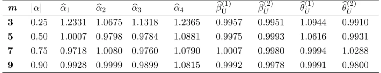
The proposed distribution to perform simulation in this particular part of study is MT-BUD. After generating samples, quality of our developed estimators was investigated. Table (1) shows accuracy of the estimators by computing ARE principle. Even though estimators are either over or under estimate, they still close to their true values. Fur-thermore, this table shows the accuracy is not affected by varying value ofm.
Table 1: Average Relative Estimate for estimated parameters compared with exact value when the density is MTBUD ats= 1, i= 1 andj=m.
m |α| αb1 αb2 αb3 αb4 βb (1) U βb (2) U θb (1) U θb (2) U 3 0.25 1.2331 1.0675 1.1318 1.2365 0.9957 0.9951 1.0944 0.9910 5 0.50 1.0007 0.9798 0.9784 1.0881 0.9975 0.9993 1.0616 0.9931 7 0.75 0.9718 1.0080 0.9760 1.0790 1.0007 0.9980 0.9994 1.0288 9 0.90 0.9928 0.9999 0.9899 1.0815 0.9992 0.9978 0.9991 0.9800
Our goal now is to calculate RE for α estimators compared to the estimator defined in (7) when the underlying distribution is MTBUD. So, variance of each estimator is required. Using Theorem (3.1) , we can find that:
var( ˆα1) = 3−α2A2i,m+ m3 A2 i,m and var( ˆα2) = 1 m(3−α 2A2 i,m) +m3 A2 i,m
. Since the difficulty in computing exactvar( ˆα3) andvar( ˆα4) , we used their estimated values. These variances
were compared with var( ˆα) =
1 12−α 2A2 s,m(16) 2 2A2 s,m(16)2 .
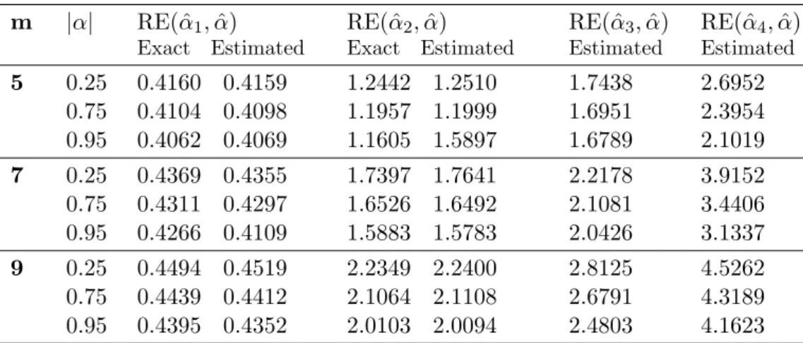
Table (2) summarizes RE of the above estimators with respect to ˆα. It shows some exact and simulated RE. It can be noted that all estimators are efficient but with one less efficient estimator that is ˆα1. However, we can increase efficiency by increasing m
at fixedα.
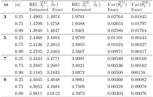
Table (3) presents RE for ˆβU(1) and ˆβU(2) with respect to ˆβU and variances for ˆθ(1)U and ˆ
θ(2)U . As noted in this table, estimators we improved in this paper are more efficient. However, we can increase efficiency by increasingm at fixed α.
Efficiency of estimators was not affected by changing values of parameters θ and β. This was seen in exact efficiency formulas which are free of these parameters as well as were clearly seen in the simulated outputs. Nevertheless, efficiency was significantly affected by changing values of the rankswhen using θb
(1) U . To see how exact variance of θb
(1)
U vary at different values ofs, with fixed m, we give general variance formula at m= 2:
var(θb (1) U ) = 1 4( 2θ2 9 − 16(3−2s)2α2θ2
2025 ). It can be noted that the variance increases as s
Table 2: Relative efficiency for ˆα1, ˆα2, ˆα3 and ˆα4 with respect to ˆα for MTBUD with s= 1 and i= 1. m |α| RE( ˆα1,α)ˆ Exact Estimated RE( ˆα2,α)ˆ Exact Estimated RE( ˆα3,α)ˆ Estimated RE( ˆα4,α)ˆ Estimated 5 0.25 0.75 0.95 0.4160 0.4159 0.4104 0.4098 0.4062 0.4069 1.2442 1.2510 1.1957 1.1999 1.1605 1.5897 1.7438 1.6951 1.6789 2.6952 2.3954 2.1019 7 0.25 0.75 0.95 0.4369 0.4355 0.4311 0.4297 0.4266 0.4109 1.7397 1.7641 1.6526 1.6492 1.5883 1.5783 2.2178 2.1081 2.0426 3.9152 3.4406 3.1337 9 0.25 0.75 0.95 0.4494 0.4519 0.4439 0.4412 0.4395 0.4352 2.2349 2.2400 2.1064 2.1108 2.0103 2.0094 2.8125 2.6791 2.4803 4.5262 4.3189 4.1623
Our last goal in this section is to investigate efficiency of the estimated population meansµ(1)X , µ(2)X , µ(1)Y andµ(2)Y with respect to SRS estimated population means .
At proposing MTBUD distribution, it is straightforward to prove that exact efficiencies forµb
(1)
X (when using ordered statistics sampling units) andµb
(1)
Y (when using concomitant sampling units)are:
RE(µb
(1)
X ,µbX) =
1
1−mm+1−1 where the produced efficiency depends on the sample size m. Particularly, for m = 3 we have RE = 2 while for m = 5 gives RE = 3 and for m = 7 gives RE = 4.
Although RE(µb(1)Y ,µbY) = 1−α21m−1 9(m+1)
. It can be noted that the minimum value of RE is always 1 by assuming α= 0 while the maximum value depends on value of m and taking |α|= 1. For m= 3 we have RE(µ(1)Y , µY) ≤ 18/17 = 1.0588, for m =5 we get RE(µ(1)Y , µY)≤27/25 = 1.08 and for m =7 we haveRE(µ(1)Y , µY)≤12/11 = 1.0909.
Table (4) reports values of RE(bµ
(2)
X ,bµX) with respect to SRS population meanµbX for some particular values ofmandα. It can be realised that the relative efficiency increases by increasing one or both ofm and α.
4.2 Estimating parameters for MTBED
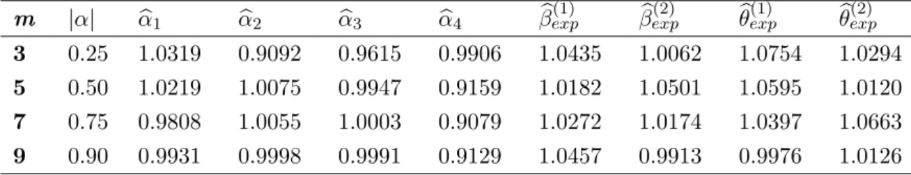
The proposed distribution to perform simulation in this particular part of study is MTBED. After generating samples, quality of our developed estimators was investigated. In Table (5), we compared estimators with arbitrarily selected true values to compute ARE. This table can show how our estimators are close to their correspondence true values.
Table (5) reports ARE for estimated parameters compared with exact value when the density is MTBED at s =1, i = 1 and j= m.
Table 3: Relative efficiency for βb
(1)
U and βb
(1)
U with respect to βbU and variances of θb
(1) U and θb
(2)
U . The proposed parameters θ= 1, β = 1 and s= 1 to computeθb
(1) U . m |α| RE(βb (1) U , βbU) Estimated Exact RE(βb (2) U , βbU) Estimated V ar(θb (1) U ) Exact V ar(θb (2) U ) Exact 3 0.25 1.4993 1.4974 1.9701 0.02764 0.01845 0.75 1.4709 1.4758 1.9488 0.02654 0.01797 0.90 1.4840 1.4647 1.9401 0.02580 0.01764 5 0.25 2.4468 2.4884 2.9789 0.01101 0.00443 0.75 2.4136 2.3913 2.8955 0.01024 0.00427 0.90 2.3705 2.3404 2.5607 0.00971 0.00417 7 0.25 3.4344 3.4771 3.9991 0.00589 0.00169 0.75 3.2887 3.2887 3.8021 0.00536 0.00162 0.90 3.1185 3.1833 3.6972 0.00500 000158 9 0.25 4.5045 4.4648 4.9861 0.00366 0.00082 0.75 4.3052 4.1684 4.7508 0.00328 0.00078 0.90 3.9811 4.0112 4.5973 0.00303 0.00076
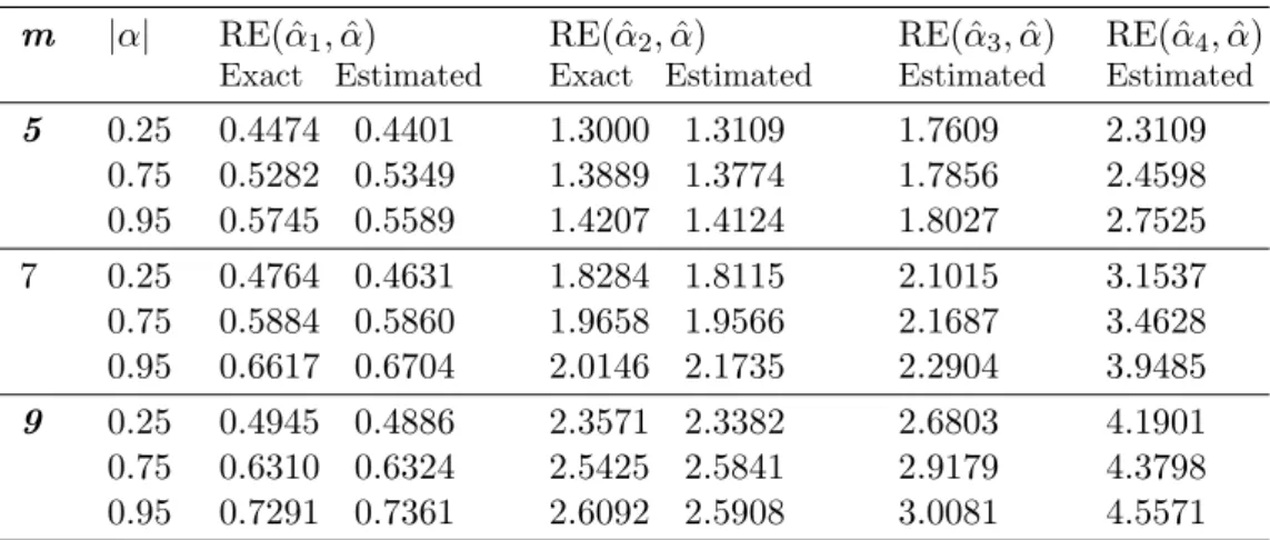
Our goal now is to calculate RE for α estimators compared to the estimator defined in (7) when the underlying distribution is MTBED. So, variance of each estimator is required. Using Theorem (3.1) , we can find that:
var( ˆα1) =
4−2αAi,m−α2A2i,m+m4
A2i,m andvar( ˆα2) =
1
m(4−2αAi,m−α 2A2
i,m+m4) A2i,m .Since the difficulty in computing exact var( ˆα3) and var( ˆα4) , we used their estimated values
to calculate RE. These variances were compared to var( ˆα) =1−α
2A2 s,m(12) 2 2A2 s,m(12)2 .
Table (6) summarizes RE of these estimators with respect to ˆα. It shows some exact and simulated RE. It can be noted that our estimators are efficient with one less efficient estimator that is ˆα1. However, we can increase efficiency by increasing the sample size
m.
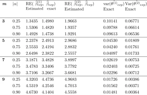
Table (7) presents RE ofβ(1)expˆ and βexp(2)ˆ with respect to ˆβexp. Importantly, there is no previous estimators forθ to compute REs so, we show variances of ˆθ(1)
exp and ˆ θexp(2). To see how exact variance of θb
(1)
exp changing at different values of s, with fixed m, we give general variance formula atm= 2:
var(θb (1) exp) = 3θ 2 16 − 29(2−2s)2α2θ2
5184 . It can be noted that the variance increases as s
in-creases.
Table 4: Relative efficiency for bµ(2)X with respect to SRS population mean µbX when MTBUD. m |α| RE(µb(2)X ,µbX) Exact 3 0.25 2.0066 0.75 2.0610 0.95 2.0998 5 0.25 3.0131 0.75 3.1225 0.95 3.2016 7 0.25 4.0197 0.75 4.1847 0.95 4.3048
Table 5: Average Relative Estimate for estimated parameters compared with exact value when the density is MTBED ats= 1, i= 1 and j=m
m |α| αb1 αb2 αb3 αb4 βb (1) exp βb (2) exp θb (1) exp θb (2) exp 3 0.25 1.0319 0.9092 0.9615 0.9906 1.0435 1.0062 1.0754 1.0294 5 0.50 1.0219 1.0075 0.9947 0.9159 1.0182 1.0501 1.0595 1.0120 7 0.75 0.9808 1.0055 1.0003 0.9079 1.0272 1.0174 1.0397 1.0663 9 0.90 0.9931 0.9998 0.9991 0.9129 1.0457 0.9913 0.9976 1.0126
meansµ(1)X , µ(2)X , µ(1)Y andµ(2)Y with respect to SRS estimated population means . At proposing MTBED distribution, the efficiency for bµ
(1)
X (when using ordered statis-tics sampling units) and µb(1)Y (when using concomitant sampling units) can be written as: RE(µb(1)X ,µbX) = 1−1 1 m Pm i=1( Pi k=1m−1k+1−1)2
where it depends only on the sample sizem. Specific examples to compute the efficiency at selected m is given next. For m = 3 we have RE = 1811 = 1.6363 while for m = 5 gives RE = 300137 and for m = 7 gives RE =
980
363 = 2.6997.
Similarly, we can investigate efficiency of µb(1)Y which is simply can be written as RE(µb(1)Y ,bµY) = 1−α21m−1
9(m+1)
. It can be noted that the minimum value of RE is al-ways 1 by assuming α= 0 while the maximum value depends on value of m and taking
Table 6: Relative efficiency for ˆα1, ˆα2, ˆα3 and ˆα4 with respect to ˆα for MTBED with s= 1 and i= 1. m |α| RE( ˆα1,α)ˆ Exact Estimated RE( ˆα2,α)ˆ Exact Estimated RE( ˆα3,α)ˆ Estimated RE( ˆα4,α)ˆ Estimated 5 0.25 0.75 0.95 0.4474 0.4401 0.5282 0.5349 0.5745 0.5589 1.3000 1.3109 1.3889 1.3774 1.4207 1.4124 1.7609 1.7856 1.8027 2.3109 2.4598 2.7525 7 0.25 0.75 0.95 0.4764 0.4631 0.5884 0.5860 0.6617 0.6704 1.8284 1.8115 1.9658 1.9566 2.0146 2.1735 2.1015 2.1687 2.2904 3.1537 3.4628 3.9485 9 0.25 0.75 0.95 0.4945 0.4886 0.6310 0.6324 0.7291 0.7361 2.3571 2.3382 2.5425 2.5841 2.6092 2.5908 2.6803 2.9179 3.0081 4.1901 4.3798 4.5571
|α| = 1. For example, if m= 3 we get RE(µ(1)Y , µY) ≤ 2423 = 1.0435, for m =5 we get RE(µ(1)Y , µY)≤ 1817 = 1.0588 and form =7 we haveRE(µ(1)Y , µY)≤ 1615 = 1.0667.
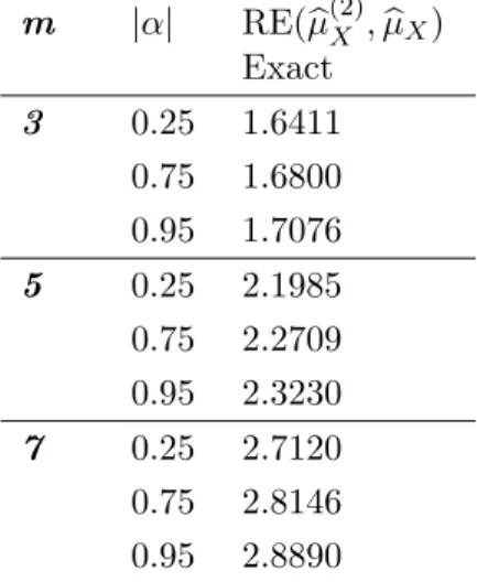
Table (8) reports values of RE(µb(2)X ,bµX) for some particular values ofm andα. It can be realised that the relative efficiency increases by increasing one ofm and α or both.
5 Conclusions and Discussion
A main benefit of RSS, as well as BVRSS, is originally to gain more information from ordered observations after quantification rather than SRS. This research gained an extra advantage from a modification on stages of BVRSS where the first stage units (which include copies of concomitant of ordered statistics) were used to achieve estimation similarly as the second stage units. An example can be stated here is when estimating α by using ˆα4 where copies of concomitant of ordered statistics were used to compute
ˆ µX(j:m).
Efficiency of our estimators was not affected by changing values of distribution pa-rameters;θandβ. We were seen this in exact efficiency formulas which are free of these parameters as well as were clearly seen in the simulated outputs. Additionally, efficiency of the estimators ˆα3 and ˆθ(1) attains its maxima when s = 1 since this rank gives the
minimum variance.
In both distribution examples that considered in this paper, we found that ˆα1 is less
efficient than SRS estimator however, it can be noted that this estimator is doing better for MTBED than MTBUD. Also, the efficiency can be improved by increasing m.
It is well known in the literature that maximum RE(µb(1)X ,µbX) (i.e using RSS units vs SRS units) can be achieved if the distribution is uniform and its value is 1
1−m−1
m+1
. In this paper, we proved that maximum RE(µb(1)X ,µbX), if the distribution is exponential, is
Table 7: Relative efficiency for βexpˆ(1) and ˆ
βexp(2) with respect to ˆβexp. The proposed value of sto compute ˆθ(1) exp is 1. m |α| RE(βb (1) exp, βbexp) Estimated exact RE(βb (2) exp, βbexp) Estimated var( ˆθ(1) exp) Exact Var( ˆθ(2) exp) Exact 3 0.25 1.3435 1.4980 1.9663 0.10141 0.06771 0.75 1.5306 1.4820 1.9357 0.09788 0.06614 0.90 1.4928 1.4738 1.9291 0.09613 0.06536 5 0.25 2.2378 2.4913 2.9686 0.04530 0.01809 0.75 2.5533 2.4194 2.8832 0.04240 0.01761 0.90 2.6498 2.3822 2.5557 0.04097 0.01733 7 0.25 3.1871 3.4828 3.8997 0.02619 0.00753 0.75 3.4783 3.3406 3.7792 0.02403 0.00725 0.90 3.7106 3.2667 3.6681 0.02296 0.00712 9 0.25 4.3203 4.4736 4.9683 0.01726 0.00386 0.75 4.5319 4.2546 4.7013 0.01562 0.00371 0.90 4.6730 4.1404 4.5558 0.01481 0.00364 equal to 1 1−1 m Pm i=1( Pi k=1m−1k+1−1) 2.
Moreover, for the concomitant of ordered statistics for MTBD, we showed that maxi-mum RE(µb(1)Y ,µbY) is equal to 1−α21m−1
9(m+1)
if the marginal distribution is uniform and is equal to 1
1−α2 m−1 12(m+1)
if the marginal distribution is exponential.
Some researchers pay attention on proving the relationship between the association parameter in MTBD and the population correlation coefficient ρ. See for example, Schucany et al. (1978) and Scaria and Nair (1999). Specifically, for MTBUD the relation is ρ =α/3 and for MTBED the relation is ρ = α/4. Therefore, we can produce many estimators for ρ by substituting estimators of α that we derived in Definition (3.1) or Definition (3.2) on these relations. Thus, a proposed estimator for MTBUD is ρb= α/3b and for MTBED is ρb= α/4.b
Acknowledgement
The authors are very thankful to the referees who gave crucial notes and suggestions which improved the earlier drafts of this paper.
Table 8: Relative efficiency for bµ(2)X with respect to SRS population mean µbX when MTBED. m |α| RE(µb(2)X ,µbX) Exact 3 0.25 1.6411 0.75 1.6800 0.95 1.7076 5 0.25 2.1985 0.75 2.2709 0.95 2.3230 7 0.25 2.7120 0.75 2.8146 0.95 2.8890
References
Abo-Eleneen, Z. and Nagaraja, H. (2002). Fisher information in an order statistic and its concomitant. Ann. Inst. Statist. Math., 54(3):667–680.
Al Kadiri, M. and Migdadi, M. (2018). Estimating morgenstern type bivariate associa-tion parameter using a modified maximum likelihood method.accepted for publication, 0.
Al-Saleh, M. and Al Kadiri, M. A. (2000). Double-ranked set sampling. Statistics and
Probability Letters, 48:205–212.
Al-Saleh, M. and Al-omari, A. (2002). Multistage ranked set sampling. Journal of
Statistical Planning and Inference, 102(2):273–286.
Al-Saleh, M. and Zheng, G. (2002). Estimation of bivariate characteristics using ranked set sampling. Australian and New Zealand Journal of Statistic, 44:221–232.
Balakrishnan, N. and Lai, C. (2009). Continuous Bivariate Distributions. 2nd ed.
Springer.
Chacko, M. and Thomas, Y. (2008). Estimation of a parameter of morgenstern type bivariate exponential by ranked set sampling. Annals of the Institute of Statistical
Mathematics, 60:273–300.
David, H. and Nagaraja, H. (2003). Order statistics. New York: Wiley.
Domma, F. and Giardano, S. (2016). Concomitants of m-generalized order statistics from generalized farlie–gumbel–morgenstern distribution family. Journal of Computational
and Applied Mathematics, 294:413–435.
Statis-tics. Atlantis Press.
Genest, C., K, G., and L, R. (1995). A semiparametric estimation procedure of depen-dence parameters in multivariate families of distributions. Biometrika, 82:543–552. Mclntyre, G. (1952). A method for unbiased selective sampling using ranked sets.
Aus-tralian Journal of Agricultural Research, 3:385–390.
Morgenstern, M. (1956). Simple examples of two-dimensional distributions. Statistik, 8:234–235.
Scaria, J. and Nair, N. (1999). On concomitants of order statistics from morgenstern family. Biometrical Journal, 41:483–489.
Schucany, W., Parr, W., and Boyer, J. (1978). Correlation structure in farile –gumbel– morgenstern distributions. Biometrika, 65:650–653.
Singh, H. and Mehta, V. (2016). Improved estimation of scale parameter of morgenstern type bivariate uniform distribution using ranked set sampling. Communications in
Statistics – Theory and Methods, 45(5):1466–1476.
Stefanescu, C. and Turnbull, B. (2009). Likelihood inference for exchangeable continuous data with covariates and varying cluster sizes; use of the farlie–gumbel–morgenstern mode. Statistical Methodology, 6:503–512.
Tahmasebi, S. and Jafari, A. (2014). Estimators for the parameter mean of morgen-stern type bivariate generalized exponential distribution using ranked set sampling.
Statistics and Operations Research Transactions, 38:1–19.
Takahasi, K. and Wakimoto, K. (1968). On unbiased estimates of the population mean based on the sample stratified by means of ordering. Ann. Inst. Statist. Math, 20:421– 428.
Wolfe, D. (2012). Ranked set sampling: Its relevance and impact on statistical inference.