Selection of our books indexed in the Book Citation Index in Web of Science™ Core Collection (BKCI)
Interested in publishing with us?
Contact [email protected]
Numbers displayed above are based on latest data collected.For more information visit www.intechopen.com Open access books available
Countries delivered to Contributors from top 500 universities
International authors and editors
Our authors are among the
most cited scientists
Downloads
We are IntechOpen,
the world’s leading publisher of
Open Access books
Built by scientists, for scientists
12.2%
122,000
135M
TOP 1%
154
Model predictive control of nonlinear processes
Author Name
x
Model predictive control
of nonlinear processes
Ch. Venkateswarlu
Indian Institute of Chemical Technology
1. Historical background
Process control has become an integral part of process plants. An automatic controller must be able to facilitate the plant operation over a wide range of operating conditions. The proportional-integral (PI) or proportional-integral-derivative (PID) controllers are commonly used in many industrial control systems. These controllers are tuned with different tuning techniques to deliver satisfactory plant performance.
Fig. 1. MPC multi-step prediction scheme.
However, specific control problems associated with the plant operations severely limit the performance of conventional controllers. The increasing complexity of plant operations
together with tougher environmental regulations, rigorous safety codes and rapidly changing economic situations demand the need for more sophisticated process controllers. Model predictive control (MPC) is an important branch of automatic control theory. MPC refers to a class of control algorithms in which a process model is used to predict and optimize the process performance. MPC has been widely applied in industry (Qin and Badgwell, 1997). The idea of MPC is to calculate a control function for the future time in order to force the controlled system response to reach the reference value. Therefore, the future reference values are to be known and the system behavior must be predictable by an appropriate model. The controller determines a manipulated variable profile that optimizes some open-loop performance objective over a finite horizon extending from the current time into the future. This manipulated variable profile is implemented until a plant measurement becomes available. Feedback is incorporated by using the measurement to update the optimization problem for the next time step. Figure 1 explains the basic idea of MPC showing how the past input-output information is used to predict the future process behavior at the current time and how this information is extended to future to track the desired setpoint trajectory. The notation y, u and Ts refer process output, control action and sample time, respectively.
2. Model predictive control scheme
Model predictive control (MPC) refers to a wide class of control algorithms that use an explicit process model to predict the behavior of a plant. The most significant feature that distinguishes MPC from other controllers is its long range prediction concept. This concept enables MPC to perform current computations to account the future dynamics, thus facilitating it to overcome the limitations of process dead time, non-minimum phase behavior and slow dynamics. In addition, MPC exhibits superior performance by systematically handling constraints violation.
Fig. 2. MPC block diagram.
The fundamental framework of MPC algorithms is common for any kind of MPC schemes. The main differences in many MPC algorithms are the types models used to represent the plant dynamics and the cost function to be minimized. The multi-step model predictive control scheme shown in Figure 1 can be realized from the block diagram represented in Figure 2.
The basic elements in the block diagram are defined as follows. An appropriate model is used to predict the process outputs,
y t i i
(
),
1,....,
N
over a future time interval known as prediction horizon, N. A sequence of control actions, u(t+j), j=1,…., m over the control horizon m are calculated by minimizing some specified objective which is a function of predicted outputs, y(t+i), set-point values, w(t+i) and control actions, u(t). The first control move, u(t) of the sequence is implemented and the calculations are repeated for the subsequent sampling instants. In order to account the plant-model mismatch, a prediction error, d(t), that is calculated based on plant measurement, y(t) and model prediction, ym(t) isused to update the future predictions.
In MPC, the control law generates a control sequence, which forces the future system response to be equal to the reference values. The system response is based on future control actions, model parameters and the actual system states. Many methods for updating the optimization problem are possible, such as estimating model parameters and/or states, inferring about disturbances etc. MPC design considers different types of process models. These include first principle models, auto regressive moving average models, polynomial models, neural network models, fuzzy models etc. The attraction for MPC is due to its capability of handling various constraints directly in the formulation through on-line optimization. A variety of model predictive control techniques have been reported for controlling the processes of various complexities.
This chapter presents different linear and nonlinear model predictive controllers with case studies illustrating their application to real processes.
3. Linear model predictive control
Linear MPC (LMPC) algorithms employ linear or linearized models to obtain the predictive response of the controlled process. These algorithms include the Model Algorithmic Control (MAC) (Richalet et al., 1978), the Dynamic Matrix Control (DMC) (Cutler and Ramaker, 1980) and the Generalized Predictive Control (GPC) (Clarke et al., 1987). These algorithms are all similar in the sense that they rely on process models to predict the behavior of the process over some future time interval, and the control calculations are based on these model predictions. The models used for these predictions have usually been derived from linear approximations of the process or experimentally obtained step response data. A survey of theory and applications of such algorithms have been reported by Garcia et al. (1989).
3.1 LMPC design
A classical autoregressive moving average (ARX) model structure that relates the plant output with the present and past plant input-output can be used to formulate a predictive model. The model parameters can be determined a priori by using the known input-output data to form a fixed predictive model or these parameters are updated at each sampling
time by an adaptive mechanism. The one step ahead predictive model can be recursively extended to obtain future predictions for the plant output. The minimization of a cost function based on future plant predictions and desired plant outputs generates an optimal control input sequence to act on the plant. The strategy is described as follows.
Predictive model
The relation between the past input-output data and the predicted output can be expressed by an ARX model of the form
y(t+1) = a1y(t) + . . . + anyy(t-ny+1) + b1u(t) +. . . + bnuu(t-nu+1) (1)
where y(t) and u(t) are the process and controller outputs at time t, y(t+1) is the one-step ahead model prediction at time t,a’s and b’s represent the model coefficients and the nu and
ny are input and output orders of the system.
Model identification
The model output prediction can be expressed as ym(t+1) = xm(t) (2) where = [1 . . . ny1 . . . nu] (3) and xm(t) = [y(t) . . . y(t-ny+1) u(t) . . . u(t-nu+1)]T (4)
with and as identified model parameters.
One of the most widely used estimators for model parameters and covariance is the popular recursive least squares (RLS) algorithm (Goodwin and Sin, 1984). The RLS algorithm provides the updated parameters of the ARX model in the operating space at each sampling instant or these parameters can be determined a priori using the known data of inputs and outputs for different operating conditions. The RLS algorithm is expressed as
(t+1) = (t) + K(t) [y(t+1) - ym(t+1)]
K(t) = P(t) xm(t+1) / [1 + xm(t+1)T P(t) xm(t+1)] (5)
P(t+1) = 1/ [P(t) - {( P(t) xm(t+1) xm(t+1)T P(t)) / (1 + xm(t+1)T P(t) xm(t+1))}]
where (t) represents the estimated parameter vector, is the forgetting factor, K(t) is the gain matrix and P(t) is the covariance matrix.
Controller formulation
The N time steps ahead output prediction over a prediction horizon is given by 1
(
)
p
y t N
y(t+N-1)+...+nyy(t-ny+N)+1u(t+N-1)+...+nuu(t-nu+N)+err(t) (6)where yp(t+N) represent the model predictions for N steps and err(t) is an estimate of the
modeling error which is assumed as constant for the entire prediction horizon. If the control horizon is m, then the controller output, u after m time steps can be assumed to be constant.
An internal model is used to eliminate the discrepancy between model and process outputs,
error(t), at each sampling instant
error(t) = y(t) - ym(t) (7)
where ym(t) is the one-step ahead model prediction at time (t-1). The estimate of the error is
then filtered to produce err(t) which minimizes the instability introduced by the modeling error feedback. The filter error is given by
err(t) = (1-Kf) err(t-1) + Kf error(t) (8) where Kf is the feedback filter gain which has to be tuned heuristically.
Back substitutions transform the prediction model equations into the following form ,1 , , 1 , 1 ,1 ,
(
)
( ) ....
(
1)
( 1)
...
(
1)
( ) ...
(
1)
( )
p N N ny N ny N ny nu N N m Ny t N
f y t
f
y t ny
f
u t
f
u t nu
g u t
g
u t m
e err t
(9)The elements f, g and e are recursively calculated using the parameters and of Eq. (3). The above equations can be written in a condensed form as
Y(t) = F X(t) + G U(t) + E err(t) (10) where Y(t) = [yp(t+1) . . . yp(t+N)]T (11) X(t) = [y(t) y(t-1) . . . y(t-ny+1) u(t-1) . . . u(t-nu+1)]T (12) U(t) = [u(t) . . . u(t+m-1)]T (13) 11 12 1( 1) 11 12 2( 1) 1 12 ( 1) ... ... : : ... ny nu ny nu N N N ny nu f f f f f f F f f f 11 21 21 1 2 3 1 2 3 0 0 ... 0 0 ... 0 . . . . . . . . . . . . . . . ... . . . ... . . . . ... . . . . ... . ... m m m mm N N N Nm g g g G g g g g g g g g E = [e1 . . . eN]T
In the above, Y(t) represents the model predictions over the prediction horizon, X(t) is a vector of past plant and controller outputs and U(t) is a vector of future controller outputs. If the coefficients of F, G and E are determined then the transformation can be completed. The number of columns in F is determined by the ARX model structure used to represent the system, where as the number of columns in G is determined by the length of the control horizon. The number of rows is fixed by the length of the prediction horizon.
Consider a cost function of the form
2 2 1 1(
)
(
)
(
1
N m p i iJ
y t i w t i
u t i
1 1( )
( )
( )
( )
( ) ( )
N m T T i iY t W t
Y t W t
U t U t
(14)where W(t) is a setpoint vector over the prediction horizon
W(t) = [ w(t+1) . . . . w(t+N)]T (15)
The minimization of the cost function, J gives optimal controller output sequence
U(t) = [GTG + I ]-1GT[W(t) - FX(t) - Eerr(t)] (16)
The vector U(t) generates control sequence over the entire control horizon. But, the first component of U(t) is actually implemented and the whole procedure is repeated again at the next sampling instant using latest measured information.
Linear model predictive control involving input-output models in classical, adaptive or fuzzy forms is proved useful for controlling processes that exhibit even some degree of nonlinear behavior (Eaton and Rawlings, 1992; Venkateswarlu and Gangiah, 1997 ; Venkateswarlu and Naidu, 2001).
3.2 Case study: linear model predictive control of a reactive distillation column
In this study, a multistep linear model predictive control (LMPC) strategy based on autoregressive moving average (ARX) model structure is presented for the control of a reactive distillation column. Although MPC has been proved useful for a variety of chemical and biochemical processes (Garcia et al., 1989 ; Eaton and Rawlings, 1992), its application to a complex dynamic system like reactive distillation is more interesting.
The process and the model
Ethyl acetate is produced through an esterfication reaction between acetic acid and ethyl alcohol 5 2 3 2 5 2 3
COOH
C
H
OH
H
O
CH
COOC
H
CH
H
(17) The achievable conversion in this reversible reaction is limited by the equilibrium conversion. This quaternary system is highly non-ideal and forms binary and ternaryazeotropes, which introduce complexity to the separation by conventional distillation. Reactive distillation can provide a means of breaking the azeotropes by altering or eliminating the conditions for azeotrope formation. Thus reactive distillation becomes attractive alternative for the production of ethyl acetate.
The rate equation of this reversible reaction in the presence of a homogeneous acid catalyst is given by (Alejski and Duprat, 1996)
1 1 1 1 2 3 4 1
(4.195
0.08815)exp(
6500.1
)
7.558 0.012
c k ck
r
k C C
C C
K
k
C
T
K
T
(18)Vora and Daoutidis (2001) have presented a two feed column configuration for ethyl acetate reactive distillation and found that by feeding the two reactants, ethanol and acetic acid, on different trays counter currently allows to enhance the forward reaction on trays and results in higher conversion and purity over the conventional column configuration of feeding the reactants on a single tray. All plates in the column are considered to be reactive. The column consists of 13 stages including the reboiler and the condenser. The less volatile acetic acid enters the 3 rd tray and the more volatile ethanol enters the 10 th tray. The steady state operating conditions of the column are shown in Table 1.
Acetic acid feed flow rate, FAc 6.9 mol/s Ethanol flow rate, FEth 6.865 mol/s Reflux flow rate, Lo 13.51 mol/s Distillate flow rate, D 6.68 mol/s Bottoms flow rate, B 7.085 mol/s Reboiler heat duty, Qr 5.88 x 10⁵ J/mol Boiling points, oK 391.05, 351.45, 373.15, 350.25 (Acetic acid, ethanol, water, ethyl acetate)
Distillate composition 0.0842, 0.1349, 0.0982, 0.6827 (Acetic acid, ethanol, water, ethyl acetate)
Bottoms composition 0.1650, 0.1575, 0.5470, 0.1306 (Acetic acid, ethanol, water, ethyl acetate)
Table 1. Design conditions for ethyl acetate reactive distillation column
The dynamic model representing the process operation involves mass and component balance equations with reaction terms, along with energy equations supported by vapor-liquid equilibrium and physical properties (Alejski & Duprat, 1996). The assumptions made in the formulation of the model include adiabatic column operation, negligible heat of reaction, negligible vapor holdup, liquid phase reaction, physical equilibrium in streams leaving each stage, negligible down comer dynamics and negligible weeping of liquid through the openings on the tray surface.The equations representing the process are given as follows.
Total mass balance Total condenser: 1 1 2 1
V
(
L
D
)
R
dt
dM
(19) Plate j: j j j j j j j jFV
V
FL
L
V
L
R
dt
dM
1 1 (20) Reboiler : n n n n nL
V
L
R
dt
dM
1 (21)Component mass balance
Total condenser : 1 , 1 , 1 2 , 2 1 , 1
)
(
)
(
i i i iV
y
L
D
x
R
dt
x
M
d
(22) Plate j:(
j i j,)
j i j, j 1 , 1i j j i j, j 1 , 1i j j i j, j i j, i j,d M x
FV yf
V y
FL xf
L x
V y
L x
R
dt
(23) Reboiler: , 1 , 1 , , ,(
n i n)
n i n n i n n i n i nd M x
L x
V y
L x
R
dt
(24)Total energy balance
Total condenser : 1 1 1 2 2 1
V
H
(
L
D
)
h
Q
dt
dE
(25) Plate j: j j j j j j j j j j j j j jFV
Hf
V
H
FL
hf
L
h
V
H
L
h
Q
dt
dE
1 1 1 1 (26) Reboiler: n n n n n n n nL
h
V
H
L
h
Q
dt
dE
1 1 (27)Level of liquid on the tray
av tray av n liq
A
MW
M
L
(28)Flow of liquid over the weir
If ( Lliq<hweir ) then Ln = 0 (29)
else 2 3
)
(
84
.
1
liq weir av av weir nL
MW
L
h
L
(30)Mole fraction normalization
1
1 1
NC i i NC i iy
x
(31) VLE calculationsFor the column operation under moderate pressures, the VLE equation assumes the ideal gas model for the vapor phase, thus making the vapor phase activity coefficient equal to unity. The VLE relation is given by
yi P = xii Pisat (i = 1,2,….,NC) (32)
The liquid phase activity coefficients are calculated using UNIFAC method (Smith et al., 1996).
Enthalpies Calculation
The relations for the liquid enthalpy h, the vapor enthalpy H and the liquid density are:
)
,
,
(
)
,
,
(
)
,
,
(
x
T
P
y
T
P
H
H
x
T
P
h
h
liq liq
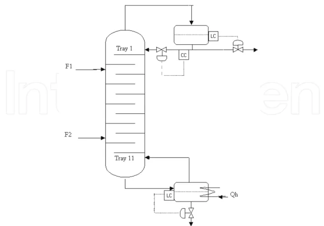
(33) Control schemeThe design and implementation of the control strategy is studied for the single input-single output (SISO) control of the ethyl acetate reactive distillation column with its double feed configuration. The objective is to control the desired product purity in the distillate stream inspite disturbances in column operation. This becomes the main control loop. Since reboiler and condenser holdups act as pure integrators, they also need to be controlled. These become the auxiliary control loops. Reflux flow rate is used as a manipulated variable to control the purity of the ethyl acetate. Distillate flow rate is used as a manipulated variable to control the condenser holdup, while bottom flow rate is used to control the reboiler holdup. In this work, it is proposed to apply a multistep model predictive controller for the main loop and conventional PI controllers for the auxiliary control loops. This control scheme is shown in the Figure 3.
Total mass balance Total condenser: 1 1 2 1
V
(
L
D
)
R
dt
dM
(19) Plate j: j j j j j j j jFV
V
FL
L
V
L
R
dt
dM
1 1 (20) Reboiler : n n n n nL
V
L
R
dt
dM
1 (21)Component mass balance
Total condenser : 1 , 1 , 1 2 , 2 1 , 1
)
(
)
(
i i i iV
y
L
D
x
R
dt
x
M
d
(22) Plate j:(
j i j,)
j i j, j 1 , 1i j j i j, j 1 , 1i j j i j, j i j, i j,d M x
FV yf
V y
FL xf
L x
V y
L x
R
dt
(23) Reboiler: , 1 , 1 , , ,(
n i n)
n i n n i n n i n i nd M x
L x
V y
L x
R
dt
(24)Total energy balance
Total condenser : 1 1 1 2 2 1
V
H
(
L
D
)
h
Q
dt
dE
(25) Plate j: j j j j j j j j j j j j j jFV
Hf
V
H
FL
hf
L
h
V
H
L
h
Q
dt
dE
1 1 1 1 (26) Reboiler: n n n n n n n nL
h
V
H
L
h
Q
dt
dE
1 1 (27)Level of liquid on the tray
av tray av n liq
A
MW
M
L
(28)Flow of liquid over the weir
If ( Lliq<hweir ) then Ln = 0 (29)
else 2 3
)
(
84
.
1
liq weir av av weir nL
MW
L
h
L
(30)Mole fraction normalization
1
1 1
NC i i NC i iy
x
(31) VLE calculationsFor the column operation under moderate pressures, the VLE equation assumes the ideal gas model for the vapor phase, thus making the vapor phase activity coefficient equal to unity. The VLE relation is given by
yi P = xii Pisat (i = 1,2,….,NC) (32)
The liquid phase activity coefficients are calculated using UNIFAC method (Smith et al., 1996).
Enthalpies Calculation
The relations for the liquid enthalpy h, the vapor enthalpy H and the liquid density are:
)
,
,
(
)
,
,
(
)
,
,
(
x
T
P
y
T
P
H
H
x
T
P
h
h
liq liq
(33) Control schemeThe design and implementation of the control strategy is studied for the single input-single output (SISO) control of the ethyl acetate reactive distillation column with its double feed configuration. The objective is to control the desired product purity in the distillate stream inspite disturbances in column operation. This becomes the main control loop. Since reboiler and condenser holdups act as pure integrators, they also need to be controlled. These become the auxiliary control loops. Reflux flow rate is used as a manipulated variable to control the purity of the ethyl acetate. Distillate flow rate is used as a manipulated variable to control the condenser holdup, while bottom flow rate is used to control the reboiler holdup. In this work, it is proposed to apply a multistep model predictive controller for the main loop and conventional PI controllers for the auxiliary control loops. This control scheme is shown in the Figure 3.
Fig. 3. Control structure of two feed ethyl acetate reactive distillation column.
Analysis of Results
The performance of the multistep linear model predictive controller (LMPC) is evaluated through simulation. The product composition measurements are obtained by solving the model equations using Euler’s integration with sampling time of 0.01 s. The input and output orders of the predictive model are considered as nu = 2 and ny = 2. The diagonal
elements of the initial covariance matrix, P(0) in the RLS algorithm are selected as 10.0, 1.0, 0.01, 0.01, respectively. The forgetting factor, used in recursive least squares is chosen as 5.0. The feedback controller gain Kf is assigned as 0.65. The tuning parameter in the
control law is set as 0.115 x 10⁻⁶. The PI controller parameters of ethyl acetate composition are evaluated by using the continuous cycling method of Ziegler and Nichols. The tuned controller settings are kc = 11.15 and
I = 1.61 x 10⁴ s. The PI controller parameters used forreflux drum and reboiler holdups are kc = - 0.001 and
I = 5.5 h, and kc = - 0.001 and I
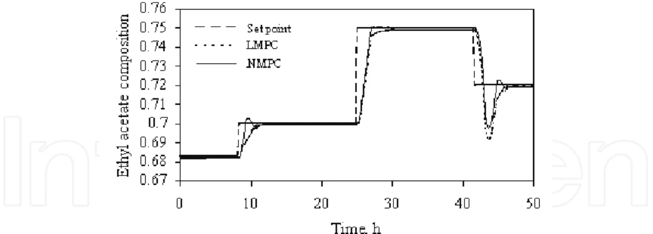
= 5.5 h, respectively (Vora and Daoutidis, 2001).The LMPC is implemented by adaptively updating the prediction model using recursive least squares. On evaluating the effect of different prediction and control horizons, it is observed that the LMPC with a prediction horizon of around 5 and a control horizon of 2 has shown reasonably better control performance. The LMPC is also referred here as MPC. Figure 4 shows the results of MPC and PI controller when they are applied for tracking series of step changes in ethyl acetate composition. The regulatory control performance of MPC and PI controller for 20% decrease in feed rate of acetic acid is shown in Figure 5. The results thus show the effectiveness of the multistep linear model predictive control strategy for the control of highly nonlinear reactive distillation column.
Fig. 4. Performance of MPC and PI controller for tracking series of step changes in distillate composition.
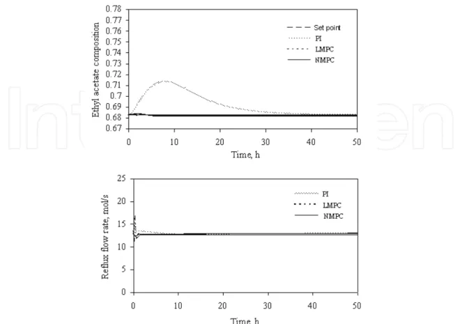
Fig.5. Output and input profiles for MPC and PI controller for 20% decrease in the feed rate of acetic acid.
Fig. 3. Control structure of two feed ethyl acetate reactive distillation column.
Analysis of Results
The performance of the multistep linear model predictive controller (LMPC) is evaluated through simulation. The product composition measurements are obtained by solving the model equations using Euler’s integration with sampling time of 0.01 s. The input and output orders of the predictive model are considered as nu = 2 and ny = 2. The diagonal
elements of the initial covariance matrix, P(0) in the RLS algorithm are selected as 10.0, 1.0, 0.01, 0.01, respectively. The forgetting factor, used in recursive least squares is chosen as 5.0. The feedback controller gain Kf is assigned as 0.65. The tuning parameter in the
control law is set as 0.115 x 10⁻⁶. The PI controller parameters of ethyl acetate composition are evaluated by using the continuous cycling method of Ziegler and Nichols. The tuned controller settings are kc = 11.15 and
I = 1.61 x 10⁴ s. The PI controller parameters used forreflux drum and reboiler holdups are kc = - 0.001 and
I = 5.5 h, and kc = - 0.001 and I
= 5.5 h, respectively (Vora and Daoutidis, 2001).The LMPC is implemented by adaptively updating the prediction model using recursive least squares. On evaluating the effect of different prediction and control horizons, it is observed that the LMPC with a prediction horizon of around 5 and a control horizon of 2 has shown reasonably better control performance. The LMPC is also referred here as MPC. Figure 4 shows the results of MPC and PI controller when they are applied for tracking series of step changes in ethyl acetate composition. The regulatory control performance of MPC and PI controller for 20% decrease in feed rate of acetic acid is shown in Figure 5. The results thus show the effectiveness of the multistep linear model predictive control strategy for the control of highly nonlinear reactive distillation column.
Fig. 4. Performance of MPC and PI controller for tracking series of step changes in distillate composition.
Fig.5. Output and input profiles for MPC and PI controller for 20% decrease in the feed rate of acetic acid.
4. Generalized predictive control
The generalized predictive control (GPC) is a general purpose multi-step predictive control algorithm (Clarke et al., 1987) for stable control of processes with variable parameters, variable dead time and a model order which changes instantaneously. GPC adopts an integrator as a natural consequence of its assumption about the basic plant model. Although GPC is capable of controlling such systems, the control performance of GPC needs to be ascertained if the process constraints are to be encountered in nonlinear processes. Camacho (1993) proposed a constrained generalized predictive controller (CGPC) for linear systems with constrained input and output signals. By this strategy, the optimum values of the future control signals are obtained by transforming the quadratic optimization problem into a linear complementarity problem. Camacho demonstrated the results of the CGPC strategy by carrying out a simulation study on a linear system with pure delay. Clarke et al. (1987) have applied the GPC to open-loop stable unconstrained linear systems. Camacho applied the CGPC to constrained open-loop stable linear system. However, most of the real processes are nonlinear and some processes change behavior over a period of time. Exploring the application of GPC to nonlinear process control will be more interesting. In this study, a constrained generalized predictive control (CGPC) strategy is presented and applied for the control of highly nonlinear and open-loop unstable processes with multiple steady states. Model parameters are updated at each sampling time by an adaptive mechanism.
4.1 GPC design
A nonlinear plant generally admits a local-linearized model when considering regulation about a particular operating point. A single-input single-output (SISO) plant on linearization can be described by a Controlled Autoregressive Integrated Moving Average (CARIMA) model of the form
A(q-1)y(t) = B(q-1)q-du(t) + C (q-1)e(t )/ (34) where A, B and C are polynomials in the backward shift operator q-1. The y(t) is the measured plant output, u(t) is the controller output, e(t) is the zero mean random Gaussian noise, d is the delay time of the system and is the differencing operator 1-q-1.
The control law of GPC is based on the minimization of a multi-step quadratic cost function defined in terms of the sum of squares of the errors between predicted and desired output trajectories with an additional term weighted by projected control increments as given by
3 2 1 2 2 1 2 3 1(
,
,
)
N[ (
| )
(
)]
N[ (
1)]
j N jJ N N N
E
y t j t w t j
u t j
(35) where E{.} is the expectation operator, y(t + j| t ) is a sequence of predicted outputs, w(t + j) is a sequence of future setpoints, u(t + j -1) is a sequence of predicted control increments and is the control weighting factor. The N1 , N2 and N3 are the minimum costing horizon, the maximum costing horizon and the control horizon, respectively. The values of N1 , N2 and N3 of Eq. (35) can be defined by N1 = d + 1, N2 = d + N, and N3 = N, respectively.Predicting the output response over a finite horizon beyond the dead-time of the process enables the controller to compensate for constant or variable time delays. The recursion of the Diophantine equation is a computationally efficient approach for modifying the predicted output trajectory. An optimum j-step a head prediction output is given by
y(t + j| t) = Gj (q-1 ) u(t + j - d - 1) + Fj (q-1 )y(t) (36)
where Gj (q-1 ) = Ej (q-1 )B(q-1), and Ej and Fj are polynomials obtained recursively solving the
Diophantine equation,
1
E
j(
q
1)
A
q
jF
j(
q
1)
(37) The j-step ahead optimal predictions of y for j = 1, . . . , N2 can be written in condensed formY =Gu + f (38)
where f contains predictions based on present and past outputs up to time t and past inputs and referred to free response of the system, i.e., f = [f1, f2, ….., fN]. The vector u corresponds
to the present and future increments of the control signal, i.e., u = [u(t), u(t+1), …….,
u(t+N-1)]T. Eq. (35) can be written as
Gu
f
w
Gu
f
w
u
u
J
T
T(39)
The minimization of J gives unconstrained solution to the projected control vector
)
(
)
(
G
G
I
1G
w
f
u
T
T
(40) The first component of the vector u is considered as the current control increment u(t), which is applied to the process and the calculations are repeated at the next sampling instant. The schematic of GPC control law is shown in Figure 6, where K is the first row of the matrix (G GT
I G)1 T.Fig. 6.The GPC control law
- + w f y(t) u(t) K Process Free response of system