THE IMPACT OF A HAUSMAN PRETEST ON THE SIZE
OF HYPOTHESIS TESTS
By
Patrik Guggenberger
April 2008
COWLES FOUNDATION DISCUSSION PAPER NO. 1651
COWLES FOUNDATION FOR RESEARCH IN ECONOMICS
YALE UNIVERSITY
Box 208281
New Haven, Connecticut 06520-8281
The Impact of a Hausman Pretest on the Size of
Hypothesis Tests
Patrik Guggenberger
Department of Economics
UCLA
First Version: November 2006
Revised: December 2007 and April 2008
I would like to thank the NSF for support under grant number
SES-0748922. I would like to thank Don Andrews, Gary
Chamberlain, Victor Chernozhukov, Phoebus Dhrymes, Ivan
Fernandez-Val, Ra¤aella Giacomini, William Greene, Jinyong Hahn,
Bruce Hansen, Jerry Hausman, Guido Imbens, Dale Jorgenson, Anna
Mikusheva, Marcelo Moreira, Ulrich Müller, Whitney Newey, Pierre
Perron, Jack Porter, Zhongjun Qu, Jim Stock, and Michael Wolf for
helpful comments. I would like to thank seminar participants at
Albany, Boston College, Boston University, Brown, Columbia,
Cornell, Georgetown, Harvard, ITAM, Madison Wisconsin, Maryland,
Minnesota, MIT, Princeton, Rochester, Syracuse, UCLA, UCSB,
Yale, and at the Cowles Econometrics conference at Yale in June 2007
at which aspects of this paper were presented. I would like to thank
the Economics Department at Harvard and the Cowles Foundation at
Yale for their hospitality while the current revision of the paper was
drafted.
Abstract
This paper investigates the size properties of a two-stage test in the linear instru-mental variables model when in the …rst stage a Hausman (1978) speci…cation test is used as a pretest of exogeneity of a regressor. In the second stage, a simple hypothesis about a component of the structural parameter vector is tested, using a t-statistic that is based on either the ordinary least squares (OLS) or the two-stage least squares estimator (2SLS) depending on the outcome of the Hausman pretest. The asymptotic size of the two-stage test is derived in a model where weak instruments are ruled out by imposing a lower bound on the strength of the instruments. The asymptotic size is a function of this lower bound and the pretest and second stage nominal sizes. The asymptotic size increases as the lower bound and the pretest size decrease. It equals 1 for empirically relevant choices of the parameter space. It is also shown that, as-ymptotically, the conditional size of the second stage test, conditional on the pretest not rejecting the null of regressor exogeneity, is 1 even for a large lower bound on the strength of the instruments.
The size distortion is caused by a discontinuity of the asymptotic distribution of the test statistic in the correlation parameter between the structural and reduced form error terms. The Hausman pretest does not have su¢ cient power against correlations that are local to zero while the OLSt-statistic takes on large values for such nonzero correlations.
Instead of using the two-stage procedure, the recommendation then is to use a
t-statistic based on the 2SLS estimator or, if weak instruments are a concern, the conditional likelihood ratio test by Moreira (2003).
Keywords: asymptotic size, exogeneity, Hausman speci…cation test, pretest, size dis-tortion
1
Introduction
This paper is concerned with the asymptotic size properties of a two-stage test where in the …rst stage, a Hausman (1978) speci…cation test is used as a pretest. As the lead example, the pretest tests exogeneity of a regressor in a linear instrumental variables (IV) model. In the second stage, a hypothesis about a component of the structural parameter vector is tested using a t-statistic based on either the ordinary least squares (OLS) or the two-stage least squares (2SLS) estimator, depending on the outcome of the pretest. An explicit formula for the asymptotic size of the two-stage test is derived in a model where weak instruments are ruled out by imposing a lower bound on the strength of the instruments. The asymptotic size is a function of the nominal size of the pretest, the nominal size of the second stage test, the number of instruments, and the lower bound on the strength of the instruments.
The speci…cation tests proposed in Hausman (1978) are routinely used as pretests in applied work, see e.g. Bradford (2003).1 As of November 2007, www.jstor.org lists about 450 citations of Hausman (1978). This number is likely a lower bound on the number of applied papers that use Hausman tests as pretests because many applied papers that use a Hausman test do so, without explicitly citing Hausman (1978) in the references. In theAmerican Economic Review alone (until 2004) there are at least 75 applied papers that use a Hausman test (about 25 of these papers were written in the years 2000-2004). Many of these papers did not cite Hausman (1978). Hausman speci…cation tests appear on the syllabus of most graduate courses in Econometrics and are discussed in any of the major Econometric textbooks, see e.g., Davidson and McKinnon (1993), Wooldridge (2002), Florens, Marimoutou, and Peguin-Feissolle (2007), and Greene (2008). However, to the best of my knowledge, no results are stated anywhere regarding the impact of the Hausman pretest on the size of a two-stage test.
First, I assess the size properties of the two stage test that uses a Hausman pretest in the …rst stage, via a Monte Carlo study in the linear IV model. An array of empirically relevant parameter choices is used for the concentration parameter 2
and the correlation between structural and reduced form error : Hansen, Hausman, and Newey (2004) provide estimates of 2 and from data sets in recently published applied papers in several top journals. Of the data sets they consider, the …rst and third quartiles of the estimated concentration parameter are 13 and 105 and the …rst and third quartiles of the estimated correlation are .07 and .47. For sample size 1Oftentimes, these speci…cation tests are also referred to asDurbin-Wu-Hausman tests based on
the papers by Durbin (1954), Wu (1973), and Hausman (1978).
Bradford (2003, p.1755-1758) conducts a Hausman pretest (based on the di¤erence of the 2SLS and OLS estimators) to test whether the regressor variables "dummy variable for pregnancy" and "number of children in the household" are exogenous in a linear regression model with left hand side variable "number of cigarettes smoked per day". The author concludes that the test "fails to reject the null at any reasonable level of signi…cance. Consequently, these two variables are treated as exogenous regressors hereafter".
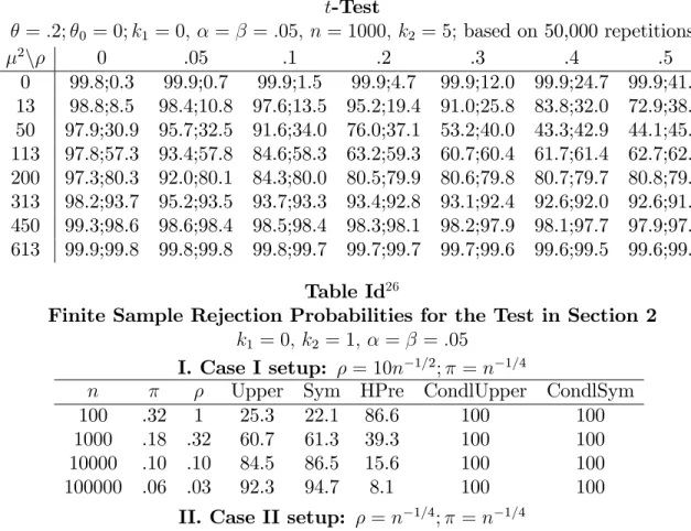
n = 1000, 5 instruments, nominal sizes of the pretest and second stage test equal to .05, the …nite sample null rejection probabilities of the two-stage test equal .87, .91, .72, .74, .15, .06 when ( 2; ) equals (13,.1), (13,.3), (13,.5), (113,.1), (113,.3), and
(113,.5), respectively. On the other hand, a simplet-test based on the 2SLS estimator has null rejection probabilities equal to .01, .06, .15, .04, .05, and .07 for these cases and thus virtually uniformly dominates the size distorted two-stage procedure in terms of null rejection properties.
Second, the paper then develops the theory to con…rm the simulation results by deriving an explicit formula for the asymptotic size of the two-stage test under strong instruments asymptotics. The asymptotic size of the two-stage test increases as the lower bound on the instrument strength, denoted by ;or the pretest size decrease.2 It is equal to 1 for empirically relevant scenarios.3 For example, for a pretest and second stage test nominal size of 5% and = :001 or :1, the asymptotic size of the symmetric two-sided test equals 1.00 and .95, respectively. For comparison, note that for the Angrist and Krueger (1991) data the strength of the instruments equals .017 and .028 for the setup with 3 and 180 instruments, respectively. See below for further discussion of this example.
As another main result, it is shown that the conditional size of the two-stage test, conditional on the Hausman pretest not rejecting the null hypothesis of exogeneity, equals 1 or is close to 1 in empirically relevant scenarios.
Sequences of nuisance parameters are characterized that lead to the highest null rejection probabilities of the two-stage test asymptotically. For sequences of correla-tions that are local to zero of order n 1=2;the Hausman pretest statistic converges
to a noncentral chi-squared distribution. The noncentrality parameter is small when the strength of the instruments is small. In this situation, the Hausman pretest has low power against local deviations of the pretest null hypothesis and consequently, with high probability, OLS based inference is done in the second stage. However, the second stage OLS based t-statistic may take on very large values under such local 2Intuitively, the terminology “strong” can be interpreted as a situation where the reduced form
coe¢ cient matrix is …xed and has full rank. In the scalar situation, it essentially means that the correlation between the instrument and the included endogenous variable is bounded away from zero. The precise de…nition, in the notation of (2.10), is that 2 = jj( 1=2 =
vjj = ( 2=n)1=2 is bounded away from zero, i.e. 2 for some lower bound on the instrument strength >0. This rules out limit distributions for estimators and test statistics obtained under the “local to zero” framework of Staiger and Stock (1997).
3The result on the asymptotic size of the two-stage test, denoted by AsySz(
0); immediately
implies an upper bound on the asymptotic con…dence size of con…dence intervals, obtained by inverting the two-stage test, given by1 AsySz( 0). It follows that the asymptotic con…dence size
of a con…dence interval based on a two-stage procedure that uses a Hausman pretest in the …rst stage, equals 0.
The Supplementary Appendix studies the asymptotic size properties of the two-stage test when weak instruments are allowed for, i.e. = 0: When weak instruments are not excluded, the space of nuisance parameters is larger, and it follows that the asymptotic size (and con…dence size) of the two-stage test (or con…dence interval) equals 1 (0).
deviations. The latter causes size distortion in the two-stage test. If, on the other hand, is kept …xed asn goes o¤ to in…nity, then the two-stage procedure has good asymptotic null rejection probabilities: If is nonzero, the Hausman pretest statistic diverges to in…nity, and in the second stage a 2SLS basedt-statistic is used. In this case, the asymptotic null rejection probability of the two-stage test equals the nominal size. If equals zero, the Hausman pretest statistic converges to a central chi-squared distribution and therefore with probability equal to1 (where denotes the nom-inal size of the pretest) at-statistic based on the OLS estimator is used in the second stage. In this case, the two-stage procedure has acceptable null rejection probability. However, this heuristic pointwise justi…cation of the two-stage procedure does not hold uniformly and the asymptotic size of the test is 1 for empirically relevant values of :
Note that in the “strong instrument scenario” considered here, a 2SLS based t -statistic has correct asymptotic size while the two-stage procedure is severely size distorted in empirically relevant scenarios. If inference on the structural parameter is the object of interest and the researcher is concerned about the null rejection probability of the inference procedure, then, based on the above …ndings, one cannot recommend the use of a Hausman test as a pretest. On the other hand, simply using a 2SLS based t-statistic is theoretically justi…ed. If, in addition, instruments are potentially weak, that is, the strength of the instruments is not bounded away from zero, my recommendation is to use any of the robust testing procedures suggested by Anderson and Rubin (1949), Moreira (2001, 2003), Kleibergen (2002), Guggenberger and Smith (2005), and Andrews, Moreira, and Stock (2006).
From the pretesting literature, it is known that pretesting may impact the size properties of two-stage tests. For example, Kabaila (1995), Andrews and Guggen-berger (2005e, AG henceforth), and Leeb and Pötscher (2005) discuss con…dence intervals (CIs) based on an estimator that can be viewed as a post-model-selection estimator based on a consistent model selection procedure. They show that the CI has asymptotic con…dence size equal to 0. AG (2005b) considers tests concerning a parameter in a linear regression model after a “conservative” model selection pro-cedure has been applied to determine whether another regressor should enter the model. They …nd that the two-stage test is extremely size distorted but can be size-corrected. This paper is closely related to the sequence of papers AG (2005a-e). As in these papers, size distortion arises here because the test statistic has an asymptotic distribution that is discontinuous in nuisance parameters of the model. The disconti-nuity in the present case arises when there is zero correlation between the structural and reduced form error terms. Earlier references on the impact of pretests include Judge and Bock (1978) and Pötscher (1991). For additional references, see the recent surveys by Dufour (2007) and Leeb and Pötscher (2008) on model selection.
This paper is related to the papers by Hahn and Hausman (2002) and Hausman, Stock, and Yogo (2005). The former paper suggests a Hausman-type (pre-)test of the null hypothesis of instrument validity. The latter paper shows that a second
stage Wald test is equally size distorted unconditionally and conditional on the Hahn and Hausman (2002) pretest not rejecting the null hypothesis of strong instruments. Another paper that is concerned with the size e¤ects of pretests is Hall, Rudebusch, and Wilcox (1996). They investigate by Monte Carlo simulation the conditional and unconditional null rejection probabilities of a second staget-test, if in the …rst stage the sample correlation between regressors and instruments is used as a pretest for instrument relevance. They …nd that the conditional size properties of the t-test, conditional on the pretest rejecting the null of instrument irrelevance, are not better than the unconditional size properties. Dhrymes (2003) and papers cited therein provide modi…ed versions of Hausman pretests.
Next, other common applications of Hausman speci…cation tests as pretests are discussed. The recent paper by Hausman and White (2006) provides a more de-tailed overview. In a panel data context, under independence of the regressors and individual speci…c e¤ects, the random e¤ects estimator is consistent and e¢ cient but inconsistent otherwise. On the other hand the …xed e¤ect estimator is consistent even if the independence assumption fails. It is to be expected that analogues of the above results hold for the size properties of a test after a Hausman pretest in this context as well. Hausman pretests have also been suggested to test for exogeneity of potential instruments. Staiger and Stock (1997) shows size distortion of the standard Hausman pretest under weakness of instruments and Hahn, Ham, and Moon (2007) introduces a modi…ed version of the Hausman pretest that is robust to weak instruments. They do not however investigate the size properties of the two-stage test which is the focus of this paper. We show in the Appendix that the conditional size of the two-stage test, conditional on the pretest not rejecting, is 1.
The remainder of the paper is organized as follows. Subsections 2.1 and 2.2 describe the model and test statistic. Subsection 2.3 reports …nite sample results using empirically relevant parameter choices. The remainder of Section 2 derives the asymptotic size results of the two-stage test when the Hausman pretest is used to test for exogeneity of a regressor. The Appendix discusses the impact on size of the Hahn, Ham, and Moon (2007) pretest.4
2
The Size of Tests After a Hausman Pretest
This section deals with the asymptotic size of the two-stage test in the linear IV model where in the …rst stage the Hausman pretest tests for exogeneity of a regressor.
4The Supplementary Appendix discusses several additional results. It shows that, for a given
bound on the instrument strength, the size correction methods of Andrews and Guggenberger (2005b) could be applied to size-correct the two-stage test. It shows that, if one allows for weak instruments, the asymptotic size of the two-stage test is 1 and size-correction is not possible. It discusses subsampling versions of the test. It shows that the same size problems of two-stage tests arise in other applications of a Hausman pretest. Finally, additional Monte Carlo results are given, including power results for the simulations in Section 2.3.
2.1
Model and De…nitions
Consider the linear IV model
y1 = y2 +X +u;
y2 = Z +X +v; (2.1)
wherey1; y2 2Rn; X 2Rn k1 fork1 0is a matrix of exogenous variables,Z 2Rn k2
fork2 1is a matrix of IVs, and( ; 0; 0; 0)0 2R1 k1 k1 k2 are unknown parameters.
LetZ = [X:Z]and k =k1+k2:Forj = 1;2; denote byyj;i; ui; vi; Xi; Zi;and Zi the
i-th rows ofyj; u; v; X; Z;andZ; respectively, written as column vectors (or scalars).
The observed data arey1; y2; X;and Z: The data (ui; vi; Zi); i= 1; :::; n;are i.i.d.
The paper investigates the asymptotic size of a two-stage test of the null hypothesis
H0 : = 0 (2.2)
where in the …rst stage a Hausman (1978) test is undertaken as a pretest. One- and two-sided alternatives are considered.
The Hausman pretest tests exogeneity of the variable y2;i.5 If the pretest rejects
the exogeneity hypothesis, then, in the second stage, H0 : = 0 is tested by using
a t-test based on the 2SLS estimator. If the pretest does not reject the exogeneity hypothesis, a t-test based on the OLS estimator is used in the second stage.
Denote by and the nominal sizes of the second stage and …rst stage test. To my knowledge, it has not been discussed in the literature what the resulting asymptotic null rejection probability of the two-stage test is as a function of and ;even under the assumption of strong identi…cation and …xed (in particular, = 0), let alone its asymptotic size. To derive the resulting asymptotic null rejection probability under these assumptions is not hard and only requires deriving the joint distribution of the pretest statistic and the possible second stage statistics. In this section, a formula for the asymptotic size of the two-stage test is derived. By de…nition, the asymptotic size of a test of the null hypothesisH0 : = 0 in the presence of nuisance parameters
2 equals
AsySz( 0) = lim sup
n!1
sup
2
P 0; (Tn( 0)> c1 ); (2.3)
whereTn( 0)is the test statistic,c1 the critical value of the test, andP ; ( )denotes
probability when the true parameters are ( ; ). The test statistics Tn( 0), critical
valuesc1 ;and parameter space for the present application are de…ned in the next
subsections. The parameter vector in our application contains as one component the correlation betweenui andvi and as second component 2 = ( 2=n)1=2;where 2
is the concentration parameter. The parameter space is modelled as a function of 5Hillier (1987) and Moreira (2001, p.7 of the July 2005 revision of the paper) provide an interesting
the strength of the instruments in subsection 2.4. By de…nition, the asymptotic size is simply the limit asn ! 1 of the exact sizesup 2 P 0; (Tn( 0)> c1 ):
See AG (2005a) and Section 2 in AG (2005d) for a detailed discussion of uniformity and the important distinction between pointwise null rejection probability and size. Uniformity over 2 which is built into the de…nition of AsySz( 0) is crucial for
the asymptotic size to give a good approximation for the …nite sample size.
2.2
Test Statistics and Critical Values
In this subsection the two-stage test statisticTn( 0)for the hypothesis testH0 : = 0
is de…ned. Denote by In the n-dimensional identity matrix. For a matrix W with n
rows, de…ne PW =W(W0W) 1W0, MW = In PW; and W? = MXW and, if no X
appears in (2.1), set W?=W:
The Hausman pretest is de…ned as
Hn= n(b2SLS bOLS)2 b V2SLS VbOLS ; (2.4) where b2SLS = y20PZ?y1=(y20PZ?y2); bOLS = y20MXy1=(y20MXy2); b V2SLS = (y20PZ?y2=n) 1b2u(b2SLS); b
VOLS = (y20MXy2=n) 1b2u(bOLS); and
b2u(bl) = n 1(y?1 y2?bl)0(y1? y2?bl) (2.5)
for l =OLS and 2SLS: Other de…nitions of Hn are possible, that replace b2u(bOLS)
by b2u(b2SLS) or vice versa. The results on the asymptotic size do not depend on
which de…nition is used, see (2.18) below. Ify2 is exogenous and the instruments are
strong then Hn !d 21 asn ! 1under assumptions given in Hausman (1978).
De…ne the t-test statistic
Tl( ) =n1=2(bl )=Vb
1=2
l (2.6)
for l=OLS and 2SLS. The standard de…nition of the two-stage test statistic is
Tn( 0) = TOLS( 0)I(Hn 21(1 )) +T2SLS( 0)I(Hn> 21(1 )); (2.7)
where, again, is the nominal size of the pretest, I is the indicator function, and
2
1(1 )the1 quantile of a chi-square random variable with one degree of freedom.
De…ne the two-stage test statisticTn( 0)as Tn( 0)orjTn( 0)jdepending on whether
The nominal 1 standard …xed critical value (FCV) test rejects H0 if
Tn( 0)> c1(1 ); (2.8)
where c1(1 ) = z1 ; z1 ; and z1 =2 for the upper one-sided, lower one-sided,
and symmetric two-sided test, respectively andz1 is the1 quantile of a standard
normal distribution.
2.3
Finite Sample Evidence
Next, the …nite sample size properties of the two-stage test are investigated in a simulation study based on parameter choices for the concentration parameter 2 and
the correlation de…ned as
2 =n 0EZ
iZi0 =Ev
2
i and =Corr(ui; vi) (2.9)
that were estimated from data sets in applied papers published in the last …ve years in theAmerican Economic Review (AER),Journal of Political Economy (JPE), and the
Quarterly Journal of Economics (QJE), see Hansen, Hausman, and Newey (2004).6 Their Table 7 is reproduced here; it reports several percentiles Q10, ..., Q90 for the concentration and correlation parameters in these data sets:
Hansen, Hausman, and Newey (2004), Table 7 Five years of AER, JPE, and QJE
# of papers Q10 Q25 Q50 Q75 Q90
2 28 8:95 12:7 23:6 105 588
22 :022 :0735 :279 :466 :555
In the simulations, the nominal sizes of the pretest and the second stage test are
= =:05:Furthermore,EZiZi0 =Ik2 and Ev
2
i = 1: This impliesjj jj=
p 2
n 1=2:
The vector is chosen to have all components equal, = 0(1; :::;1)0 2 Rk2 for 0 2 R. The vector (ui; vi; Zi) is chosen as i.i.d. normal with zero mean and unit
variances andZi is independent of ui and vi: The asymptotic results do not depend
on k1; the number of included exogenous variables, and therefore k1 = 0 in the
simulations.
Two Monte Carlo experiments based on the information in Table 7 of Hansen, Hausman, and Newey (2004) are implemented.
In the …rst experiment, the values of 2 and are …xed at the estimated median
values over the data sets, namely 2 = 23:6 and = :279: Empirical null rejection probabilities of the two-stage test are reported for various values of the sample sizen
6The concentration parameter 2equalsn 0EZ
iZi0 =Ev2i when there are no included exogenous variables. In general, the concentration parameter is de…ned asn 2
2 where 2 is de…ned in (2.10).
and the number of instrumentsk2;namelyn 2 f100;1000;10000gandk2 =f1;5;20g:
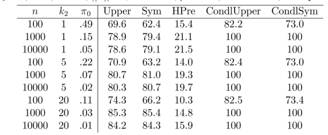
In Table Ia below, columns 4 and 5 with headings “Upper” and “Sym” report these …nite sample null rejection probabilities for upper and symmetric two-stage tests. Column 6 with heading “HPre” reports null rejection probabilities of the Hausman pretest. Finally, columns 7 and 8 with headings “CondlUpper” and “CondlSym” report conditional probabilities of rejecting the null hypothesis of the second stage test, conditional on the Hausman pretest not rejecting the pretest null hypothesis.
For all con…gurations, the two-stage test overrejects severely, with null rejection probabilities in the range[:62; :85]. The pretest null hypothesis is only rejected with probabilities ranging roughly between 10% and 20% even though =:279. However, conditional on not rejecting the pretest null hypothesis and thus using an OLS based
t-statistic in the second stage, the null rejection probabilities equal 100% in most scenarios. The OLS based t-statistic takes on very large values under the failure of the pretest null hypothesis while the Hausman pretest does not.
Insert Table Ia about here
In the second experiment, the sample size and the number of instruments are …xed at n = 1000; k2 = 5 and various values of the concentration parameter 2
and are considered that cover the whole range of values reported in Hansen, Hausman, and Newey (2004), namely 2
2 f0;13;50;113;200;313;450;613g and
2 f0; :05; :1; :2; :3; :4; :5; :6g: Therefore, the results cover all the cases of combi-nations of 2 and that were found in the applied papers in the last …ve years in AER, JPE, and QJE considered in the table above. For each such combination, Table Ib below reports null rejection probabilities of the symmetric two-stage test and of the symmetric t-test based on the 2SLS estimator. The results imply that in terms of null rejection probabilities, simply using the one-stage t-test, is the better of the two methods. In situations, where the two-stage test has good null rejection proba-bilities (the cases where = 0 or ( :3 and 2 200)), the same is true for the one-stage t-test. However, in all other situations the two-stage test overrejects, of-tentimes severely, while the one-stage test has relatively good size properties(except when :5 and 2 13). For example, for the cases (:1 :4 and 2 13) the null rejection probabilities of the two-stage test fall into the interval [:84;1:00] while the corresponding interval for the one-stage test is[0; :1]. For =:1the null rejection probability of the two-stage test is :87when = 13 and :38 when = 613 while for the one-stage test, the corresponding probabilities are:01and :05.
Insert Table Ib about here
In the next subsections, the theoretical evidence is provided to support the results of the …nite sample simulations. The next subsection de…nes the space of nuisance parameters. Finally, the asymptotic size of the two-stage test is derived.
2.4
Parameter Space
In this subsection, the parameter space of the nuisance parameter vector is de-…ned. Following AG (2005a), the parameter has three components: = ( 1; 2; 3):
The points of discontinuity of the asymptotic distribution of the test statistic of in-terest are determined by the …rst component, 1: The parameter space of 1 is 1:
The second component, 2;of also a¤ects the limit distribution of the test statistic,
but does not a¤ect the distance of the parameter to the point of discontinuity. The parameter space of 2 is 2: The third component, 3; of does not a¤ect the
limit distribution of the test statistic. The parameter space for 3 is 3( 1; 2);which
generally may depend on 1 and 2:
The “strength of the instruments”, 2 = jj( 1=2 =
vjj de…ned in (2.10) below;
a¤ects the limit distribution of the test statistics discontinuously at the point 0 of no identi…cation, see the Supplementary Appendix, Section 6. Because the data evidence in Hansen, Hausman, and Newey (2004) suggests that extremely weak identi…cation is rather the exception, a lower bound on the strength of the instrumentsjj( 1=2 = vjj
is imposed for some >0: Weak instruments as in Staiger and Stock (1997), that would correspond to = 0, are therefore ruled out. By imposing a lower bound,
jj( 1=2 = vjjno longer a¤ects the limit distribution discontinuously, but continuously,
see below.
Assume that f(ui; vi; Xi; Zi) : i ng are i.i.d. with distribution F: De…ne the
vector of nuisance parameters = ( 1; 2; 3); by
1 = ; 2 =jj( 1=2 = vjj; and 3 = (F; ; ; ); where 2 u =EFu2i; 2 v =EFv2i; =CorrF(ui; vi); =QZZ QZXQXX1 QXZ; and Q= QXX QXZ QZX QZZ =EFZiZ 0 i; (2.10)
andjj jjdenotes Euclidean norm. The parameter 1 measures the degree of endogene-ity of y2:7 The parameter 2 measures the strength of the instruments. It is related
to the concentration parameter 2 (de…ned above for the particular casek
1 = 0) by 2 =n 1=2 : Let
1 = [ 1;1]; 2 = [ ; ] (2.11)
7Note that we choose the above parameterization for because it allows for veri…cation of
As-sumption B in AG (2005a) in the most parsimonious way. AsAs-sumption B allows us to calculate the asymptotic size of the two-stage test for di¤erent speci…cations of ;in particular of 2: The latter
is important to assess the relevance of our …ndings on asymptotic size for empirical applications, see the discussion around Table II below.
Note that in AG (2005a-e) the speci…cation for has always been chosen such that when 1times nr diverges to in…nity, the “standard FCV” asymptotic distribution is obtained. In this example, whenn1=2j 1j ! 1; y2is not exogenous. Instead, the “standard”Hausman (1978) resultHn!d 21
for some 0 < < < 1: The technical details of the de…nition of 3 = 3( 1; 2)
are given in the Appendix, see (3.1).8 Finally, de…ne the parameter space of as
=f = ( 1; 2; 3) : 1 2 1; 2 2 2; 3 2 3( 1; 2)g: (2.12)
2.5
Asymptotic Distributions and Size
In this subsection, the asymptotic distribution of the test statistic is derived under certain parameter sequences f n;hg de…ned below. Then the asymptotic size of the test is determined.
Let R1=R[ f 1g: De…ne
H = fh= (h1; h2)2R21 :9 f n = ( n;1; n;2; n;3)2 :n 1g
such that n1=2 n;1 !h1 and n;2 !h2g: (2.13)
It follows that
H=H1 H2 =R1 [ ; ]: (2.14)
Two cases are dealt with separately. Case I hasjh1j<1while Case II hasjh1j=1:
In Case I, ! 0 and thus var(uivi)=( 2u 2v) ! 1, see (3.2). In Case I, y2 is only
“weakly endogenous” while in Case II it is “strongly endogenous”.
De…nition of f n;hg : For h = (h1; h2) 2 H; let f n;hg denote a sequence
of parameters with components n;h;1; n;h;2; and n;h;3; n;h = ( n;h;1; n;h;2; n;h;3)0;
where n;h;1 = CorrFn(ui; vi); n;h;2 =jj( 1=2 n n=(EFnv 2 i) 1=2 jj; for n = EFnZiZ 0 i EFnZiX 0 i(EFnXiX 0 i) 1 EFnXiZ 0 i; s.t. n1=2 n;h;1 ! h1; n;h;2 !h2; and n;h;3 = (Fn; n; n; n)2 3( n;h;1; n;h;2): (2.15) As Theorem 1 below shows, the highest asymptotic null rejection probability of the test is realized along some sequence of the typef n;hg:It is therefore enough to study
8In a panel data model,
yit=xit +ci+uit
with individual speci…c e¤ectsci;a Hausman pretest is often used to test the key assumption needed to justify the use of a random e¤ects estimator, namely E(cijxi) = 0; where xi = (xi1; :::; xiT) and T is the time series dimension of the panel. The …xed e¤ects estimator based on the within transformation,yeit=yit yi;whereyidenotes the time average,eyit=exit +ueit(where the notation forexitandueitshould be clear), is justi…ed even when this assumption fails. An assumption needed for the …xed e¤ect estimator is thatrank(PTt=1Exe0
itxeit)is maximal. There is a problem if for ani; xitdoes not vary much over time, and thereforeexit 0:In the panel model, the analogues to 1and 2 are parameters that measure the failure ofE(cijxi) = 0and “rank(PTt=1Eex0itexit)is maximal”, respectively.
the asymptotic rejection rates along sequencesf n;hg:Under any sequencef n;hgfor whichCorrFn(ui; vi)! ; the following convergence result holds
0 @ (n 1Z?0Z?) 1=2n 1=2Z?0u= u (n 1Z?0Z?) 1=2n 1=2Z?0v= v n 1=2(u0v EFnu0v)=( u v) 1 A!d 0 @ u;v; uv; 1 A N(0; V Ik2 0 00 1 + 2 ) forV = 1 1 ; (2.16) where u; ; v; 2Rk2;
uv; 2R. See AG (2005c, eq. (2.15)) for similar statements.9
Next the limit distribution of the test statistic Tn( 0) is derived under sequences
n;h: To do so, (2.16) and derivations from AG (2005c, Sections 2.3 and 4.1.2) are
used. For Case I and h = ( 1;h; :::; 4;h)0; h= (h1; h2)0
0 B B @ n 1=2y0 2PZ?u=( u v) n 1=2y0 2MXu=( u v) n 1y20PZ?y2= 2v n 1y0 2MXy2= 2v 1 C C A!d h = 0 B B @ h2s0k2 u;0 h2s0k2 u;0+ uv;0+h1 h2 2 h2 2+ 1 1 C C A; (2.17) where sk2 2R
k2 is an arbitrary vector with
jjsk2jj= 1. Therefore, 0 B B B B @ T2SLS( 0) TOLS( 0) Hn b2u(b2SLS)= 2u b2 u(bOLS)= 2u 1 C C C C A!d h = 0 B B B B @ s0 k2 u;0 (1 +h2 2) 1=2 2;h (1 +h2 2)[s0k2 u;0 h2(1 +h 2 2) 1 2;h]2 1 1 1 C C C C A: (2.18) for 0
h = ( 1;h; :::; 5;h):10 Case II is dealt with in the Appendix. In Case II, the
pretest statistic goes o¤ to in…nity, Hn !p 1;and thus w.p.a.1, T2SLS( 0) is used in
the second stage. BecauseT2SLS( 0)!dN(0;1), there is no size-distortion under the
strong endogeneity of Case II. We have
Tn( 0)!dJh; (2.19)
where Jh; by de…nition, is the distribution of
h = 2;hI( 3;h 21(1 )) + 1;hI( 3;h > 21(1 )): (2.20)
9Condition (3.2) in the de…nition of
3( 1; 2)ensures that we get the zero entries in the
covari-ance matrix of the asymptotic distribution of( 0u; ; 0v; ; uv; )and also that the right lower entry
( u2 v2)var(uivi)in the covariance matrix equals1 + 2.
10Because
3;h= (1+h22) 1[s0k2 u;0 h2 uv;0 h2h1]
2ands0
k2 u;0 h2 uv;0 h2h1 N( h2h1;1+
h2
2);the limit distribution ofHnis 21(h21h22(h22+ 1) 1):Therefore,Hn!d 21ifh1= 0;that is under
exogeneity and strong instruments, we obtain Hausman’s (1978) result as a subcase. If h2h1 6= 0
The distributionJh depends on the nominal size of the pretest. For notational sim-plicity, this dependence is suppressed. The derivations above imply that Assumption B in AG (2005a) holds withr = 1=2:
Next, an explanation is provided for the size distortion of the two-stage test. Simply to gain some intuition, we evaluate the formulas in (2.18) at h2 = 0, i.e.
the unidenti…ed case. Strictly speaking, this is not allowed, because forh2 = 0weak
instrument asymptotics could apply. However, by continuity, the same intuition given below applies for small values for h2 rather than h2 = 0: This is con…rmed by the
theoretical results stated below Theorem 1.
The formulas in (2.18) evaluated at h2 = 0 read
T2SLS( 0) !ds0k2 u;0;
TOLS( 0) !d uv;0+h1; and
Hn !d(s0k2 u;0)
2 2
(1): (2.21)
It follows that in this situation, the Hausman pretest rejects with probability equal to :When the Hausman test does not reject the pretest hypothesis (which happens with probability1 ) and thus the OLS basedt-statistic is used in the second stage, the maximal asymptotic rejection probability for the null H0 : = 0 equals 1. The
latter is seen by pickingh1 very large or very negative depending on the type of test.11
Note that picking a large nominal pretest size does not solve this problem. While picking a large reduces the probability at which OLS based inference is performed in the second stage, it does not lower the conditional size of the second stage test, conditional on not rejecting the pretest null hypothesis. In particular, assume the nominal size of the pretest is chosen such that = n ! 1. While the probability of using OLS based inference in the second stage goes to zero (and the two-stage test essentially boils down to the much simpler one-stage test that always uses a t -statistic based on 2SLS), whenever OLS based inference is used in the second stage, the conditional size of the test equals 1. So whenever one tries to gain power by using OLS based inference, the size of the test is completely distorted.
The typically more powerful OLS based inference in the second stage comes at the price of extreme size distortion. If, for example, = =:05;then the unconditional asymptotic size for the upper two-stage FCV test is at least 97.5%: With probability
1 ; a t-statistic based on OLS is used and always rejects the null (for h1 large
enough) and with probability ;at-statistic based on 2SLS is used which rejects the null with probability 1/2. Intuitively, the pretest does not pick up the local invalidity of the exogeneity assumption, =n 1=2h
1. On the other hand, the mean of the limit
distribution of the OLS based t-statistic is a¤ected which leads to overrejection. 11Consider, for example, the case of an upper one-sided test. For every " > 0 there exists a
h1=h1(")such that P( uv;0+h1 > z1 )>1 ": Therefore, under the sequence n =n 1=2h1;
The next theorem gives an explicit formula for the asymptotic size AsySz( 0) of
the two-stage test of H0 : = 0 based onTn( 0). The results apply to upper, lower
one-sided, and symmetric two-sided versions of the test with h de…ned as h; h;
and j hj; respectively.
Theorem 1 For upper, lower, and symmetric FCV tests based on Tn( 0)of nominal
size , the AsySz( 0) equals suph2HP( h > c1(1 )):
The proof follows from Theorem 1(a) in AG (2005a). Note that the asymptotic sizes depend on the pretest size and on :For notational simplicity, this dependence is suppressed. Note that the results do not depend on k1:
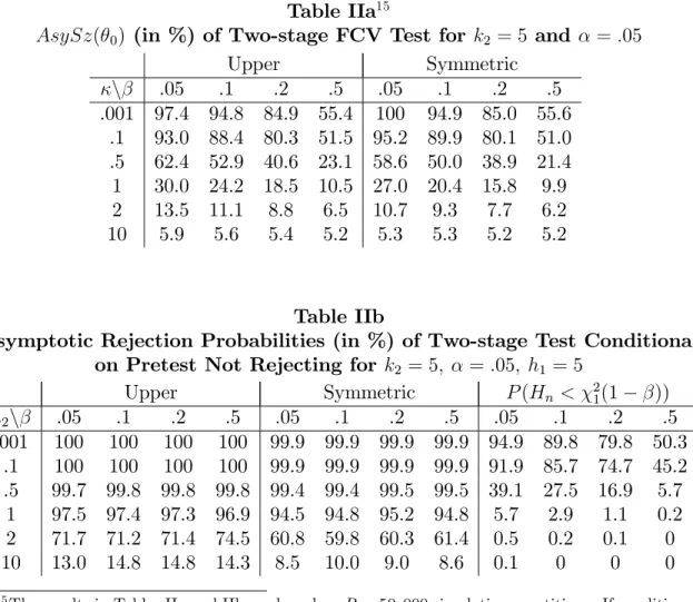
Table IIa contains information on the asymptotic size of the two-stage test when
k2 = 5 and = :05 for various values of and , namely 2 f:001; :1; :5;1;2;10g
and 2 f:05; :1; :2; :5g:12 Here and in the tables below, only results on upper and symmetric tests are reported. Results for lower (and equal-tailed) tests are virtually identical to the upper (and symmetric) ones. Note that a one-stage t-test based on the 2SLS estimator has asymptotic size equal to 5% whenever >0:
Insert Table IIa about here
Naturally,AsySz( 0)is decreasing in both and :Table IIa shows thatAsySz( 0)
by far exceeds the nominal size for small numbers of and : For example, when
=:1 and = :05 then the asymptotic size equals .93 and .95 for upper and sym-metric tests, respectively. On the other hand, when = 10 and = :05 then the asymptotic size equals .06 and .05 for upper and symmetric tests, respectively, and therefore basically equals the nominal size of the test. For = :05 the symmetric test has asymptotic size equal to 1 for small lower bounds on the strength of the instrument.
To gain further insight, the asymptotic probability of the event “pretest does not reject the pretest null hypothesis” and the conditional probability of the event “test rejects the null hypothesis” conditional on the pretest not rejecting the pretest null hypothesis, are investigated. Table IIb contains the results for the case whereh1 = 5
and various values of h2 and pretest nominal sizes : For h2 1; this conditional
rejection probability is very close to or equal to 1 for both upper and symmetric tests for all nominal sizes considered. Picking a large decreases the asymptotic size of the two-stage test by more often using 2SLS based inference in the second stage, but it does not decrease the size problems of the test if OLS based inference is used in the second stage. The pretest does not detect a violation of the pretest null 12In the simulations, = 1000:Hansen, Newey, and Hausman (2004, Table 1) reports estimated
concentration parameters 2 for the Angrist and Krueger (1991) data for two di¤erent setups with
number of instruments equal to 3 and 180, respectively. The estimated concentration parameters are 2 = 95:6 and257, respectively. For the sample size n= 329;509 this implies
2 = :017 and :028; respectively.
hypothesis, however the second stage t-statistic based on the OLS estimator takes on very large values. The probability of not rejecting the pretest null hypothesis,
P(Hn < 21(1 )); is of course decreasing in and h2 1: For = :05 and
h2 = :1; it equals .92. The asymptotic size AsySz( 0) is large because, the pretest
null hypothesis is not rejected with a large probability and conditional on this, the second stage t-test based on OLS almost certainly rejects the null.
3
Appendix
De…nition of the set 3( 1; 2) :De…ne
3( 1; 2) =f(F; ; ; ) : EFui =EFvi = 0; EFu2i = 2 u; EFv2i = 2 v; EFZiZ 0 i =Q= QXX QXZ QZX QZZ ;
for some 2u; 2v >0; pd Q2Rk k; & 2Rk2 that satisfy
CorrF(ui; vi) = 1; jj 1=2 = vjj= 2 for =QZZ QZXQXX1 QXZ; ; 2Rk1; E FuiZi =EFviZi = 0; EF(u2i; vi2; uivi)ZiZ 0 i = ( 2u; 2v; u v )Q; EF(u2iviZi) =EF(uivi2Zi) = 0; var(uivi)=( 2u 2 v) = 1 + 2 1; min(EFZiZ 0 i) M 1; E F jui= uj2+ ; jvi= vj2+ ; juivi=( u v)j2+ 0 M; & EF jjZiui= ujj2+ ; jjZivi= vjj2+ ; jjZijj2+ 0 Mg (3.1)
for some constants > 0 and M < 1; where “pd” denotes “positive de…nite.” The restrictions in 3( 1; 2) are similar to those in AG (2005c) and comprise exogeneity
restrictions on Z; moment restrictions that ensure the validity of central limit the-orems and, for simplicity, conditional homoskedasticity is assumed. The additional conditions EF(u2iviZi) =EF(uivi2Zi) = 0 and var(uivi)=( 2u 2 v) = 1 + 2 ; (3.2) where =CorrF(ui; vi);ensure that under exogeneity and strong instrumentsb2SLS
bOLS is asymptotically uncorrelated with bOLS. Hausman (1978) exploits the latter
property when deriving the asymptotic variance ofb2SLS bOLS when showing that
H !d 21 under strong instruments and exogeneity of y2: Su¢ cient conditions for
(3.2) are, for example, independence of (ui; vi)and Zi and joint normality of (ui; vi)
with zero mean.
Limit distribution of test statistic in Case II: Under sequences f n;hg for whichCorrFn(ui; vi)! and h= (h1; h2)0 with jh1j=1 the following holds jointly
0 B B @ n 1=2y0 2PZ?u=( u v) n 1=2[y0 2MXu EFnu0v]=( u v) n 1y0 2PZ?y2= 2v n 1y20MXy2= 2v 1 C C A!d h = 0 B B @ h2s0k2 u; h2s0k2 u; + uv; h2 2 h2 2+ 1 1 C C A (3.3) and 0 B B B B @ T2SLS( 0) TOLS( 0) Hn b2u(b2SLS)= 2u b2 u(bOLS)= 2u 1 C C C C A!d h = 0 B B B B @ s0 k2 u; h1 1 1 1 2=(h2 2+ 1) 1 C C C C A : (3.4)
3.1
Pretesting Instrument Exogeneity
In this application, the Hausman speci…cation test is used as a pretest to test for instrument exogeneity. More precisely, the instruments are decomposed into Z = (W; S); whereW hask21 andS hask22 columns andk2 =k21+k22: The instruments
S are potentially invalid, that is correlated with u, while the instruments W are assumed to be valid. The Hausman pretest tests whether S are valid instruments. If the pretest is rejected, then in the second stage, the hypothesis H0 : = 0 is tested
by using a t-statistic based on only the instruments W. Otherwise, a t-statistic is used based on all instruments Z. In an application, one could think of W and S as weak and strong instruments, respectively.
We show that the conditional size of the two-stage test, conditional on the Haus-man pretest not rejecting the pretest null hypothesis, is 1 asymptotically. Similar results can be shown for the (unconditional) asymptotic size.
To test orthogonality of the instrumentsS; two di¤erent versions of a pretest are being considered. The …rst one, denoted again by Hn; is a standard version of a
Hausman test and the second one, denoted byH4 is the version of the Hausman test
introduced in Hahn, Ham, and Moon (2007) using their notation. In this subsection, for ease of presentation, there are no included exogenous variables and is again scalar. The formulas are
Hn = n(bW bZ)2 b VW VbZ ; H4 = eu2(y1 y2bZ)0W[W0W W0y2(y20PZy2) 1y20W] 1W0(y1 y2bZ); e2u = n 1(y 1 y2bZ)0MZ(y1 y2bZ); (3.5)
where bW and VbW are de…ned analogously to the 2SLS expressions in (2.5), when
the estimators are based only on the instruments W; likewise, bZ and VbZ denote
what was previously denoted by b2SLS and Vb2SLS in (2.5). Similar straightforward
modi…cations to the notation are used for other expressions, e.g. TW( 0)andTZ ( 0)
are used in place of T2SLS( 0) when the statistic is based on instruments W or Z,
respectively. As shown by Hahn, Ham, and Moon (2007), H4 is asymptotically 2
even when instruments are weak. This is not true for Hn, see Staiger and Stock
(1997):
For simplicity, assume k22= 1; ESi = 0;andESiWi = 0k21, where0k denotes ak -dimensional vector of zeros. That is, there is only one (potentially) strong instrument, it has mean zero and is uncorrelated with the other instruments. Simply view Si as
the residual of a strong instrument that is being regressed on the instrumentsWi:
Denote by f n;hg a sequence of parameters with components n;h;1; n;h;2;
and n;h;3; such that
n;h;1 = (jj((EFnZiZ 0 i) 1=2 n=(EFnv 2 i) 1=2 jj; CorrFn(ui; Si)); n;h;2 = ( n;h;1; CorrFn(ui; vi)); n 1=2 n;h;1 !h1; n;h;2 !h2; and (3.6)
n;h;3satisfying similar restrictions to those in (6.14) includingEFnWiSiu 2 i =EFnWiSiu 2 i = 0k21;and varFnSiui=(EFnS 2 iEFnu 2
i) = 1 +Corr2Fn(Si; vi). With these assumptions,
un-der any sequence f n;hg; the following convergence result similar to (6.26) holds
(n 1Z0Z) 1=2n 1=2((W0u)0; S0u ES0u)0= u (n 1Z0Z) 1=2n 1=2Z0v= v !d u;h2 v;h2 N(0; Ik2;h22 h23Ik2 h23Ik2 Ik2 ) for Ik2;h22 = Ik21 0 0 1 +h2 22 : (3.7)
For simplicity, it is only shown that conditional on the Hausman pretest (based onHn or H4) not rejecting the pretest null hypothesis of instrument exogeneity, the
asymptotic size of the two-stage FCV procedure equals 1. It turns out that, to show this, only requires looking at a particular scenario modelled by
y2 =n 1=4 SS+v
n1=2 n;h;1;2 !h12 …nite (3.8)
for a …xed nonzero number S:13 The coe¢ cients on the weak instruments are
mod-elled as zero while the coe¢ cient on the strong instrument shrinks to zero at rate
n 1=4. The instruments are strong in the sense that the concentration parameter
goes o¤ to in…nity. Because n1=2 n;h;1;2 !h12 for h12 …nite, the instrument is weakly
endogenous. Model (3.8), when viewed as a sequence f n;hg, has h = (h1; h2) with
h1 = (1; h12) and h2 = (0;0; h23):
Using (3.7) it follows that under (3.8) for h = ( 1;h; :::; 6;h)0
0 B B B B B B @ n 1=4y02PZu=( u S) y0 2PWu=( u v) n 1=2y0 2PZy2= 2S y0 2PWy2= 2v b2u(bZ)= 2u b2u(bW)= 2u 1 C C C C C C A !d h = 0 B B B B B B @ S( u;h2;k2 +h12) 0 v;h2;1:k21 u;h2;1:k21 2 S 0 v;h2;1:k21 v;h2;1:k21 1 1 2h23 2;h= 4;h+ ( 2;h= 4;h)2 1 C C C C C C A ; (3.9)
where u;h2;k2 denotes thek2-th entry in u;h2 and v;h2;1:k21 and u;h2;1:k21 denote the …rst k21 entries of v;h2 and u;h2, respectively. The statisticsbW and VbW inHn are of higher order than the statisticsbZ and VbZ and the latter hence do not matter for
the asymptotic distribution of Hn in model (3.8). Likewise, in H4; W0W is of higher
order than W0y
2(y02PZy2) 1y20W and the latter term can be neglected for the limit
theory. Finally, e2u= 2
u !p 1:By (3.9), we therefore have in model (3.8)
0 @ TZ ( 0) Hn H4 1 A!d h = 0 @ u;h2;k2 +h12 2 2;h 4;h=( 2 4;h 2h23 2;h 4;h+ 2 2;h) 0 u;h2;1:k21 u;h2;1:k21 1 A: (3.10) 13The result of conditional size equal to 1 asymptotically can be shown by looking at many di¤erent
sequences of the nuisance parameters. Here, I pick one particularly simple choice that makes the analysis easy. Assume, in addition, that 2
v = EFnv 2
i and 2S = EFnS 2
i are nonzero and do not depend onn:
Let h = ( 1;h; 2;h; 3;h)0: Note that 1;h and 2;h are independent, because 2;h and
4;h only depend on v;h2;1:k21 and u;h2;1:k21 and by (3.7) those random variables are independent of u;h2;k2. Therefore, asymptotically, conditional on the pretest based onHn not rejecting, TZ ( 0) is distributed as u;h2;k2 +h12: Hence, pickingh12 large enough (or small enough for lower one-sided tests), it is clear that the conditional size of the two-stage test, conditional on the pretest based onHn not rejecting the pretest
null hypothesis, is 1 asymptotically. The same argument holds for the two-stage test with the pretest based on H4: The limit distribution of H4 is a chi-squared withk21
References
Anderson, T.W. and H. Rubin (1949): “Estimators of the parameters of a single equation in a complete set of stochastic equations,”The Annals of Mathematical Statistics 21, 570–582.
Andrews, D. W. K. and P. Guggenberger (2005a): “Asymptotic Size and a Problem with Subsampling and with the m out of n Bootstrap,”unpublished working paper, Dept. Econom., Yale.
— — — (2005b): “Hybrid and Size-Corrected Subsampling Methods,”unpublished working paper, Dept. Econom., Yale.
— — — (2005c): “Applications of Subsampling, Hybrid and Size-Correction Meth-ods,”Cowles Foundation Discussion Paper 1608.
— — — (2005d): “Validity of Subsampling and “Plug-in Asymptotic” Inference for Parameters De…ned by Moment Inequalities,”Cowles Foundation Discussion Paper 1620.
— — — (2005e): “Invalidity of subsampling inference based on post-consistent model selection estimators,”manuscript in preparation, Dept. Econom., Yale.
Andrews, D.W.K., M.J. Moreira, and J.H. Stock (2006): “Optimal invariant similar tests for instrumental variables regression,”Econometrica, 74, 715–752.
Angrist, J. and A. Krueger (1991): “Does Compulsory School Attendance A¤ect Schoolings and Earnings?,”Quaterly Journal of Economics, 106, 979–1014. Bradford, W.D. (2003): “Pregnancy and the Demand for Cigarettes,”American
Economic Review, 93, 1752–1763.
Davidson, R. and J.G. MacKinnon (1993): “Estimation and Inference in Economet-rics,” Oxford University Press, New York.
Dhrymes, P.J. (2003): “Tests for Endogeneity and Instrument Suitability,” unpub-lished working paper, Dept. Econom., Columbia.
Dufour, J.M. (2007): “Model Selection,” New Palgrave Dictionary of Economics, 2nd Edition, forthcoming.
Durbin, J. (1954): “Errors in Variables,”Review of the International Statistical Institute, 22, 23–32.
Florens, J.P., V. Marimoutou, and A. Peguin-Feissolle (2007): “Econometric Mod-eling and Inference,” Cambridge University Press, Cambridge, U.K.
Greene, W. (2008): “Econometric Analysis,” Prentice Hall, Englewood Cli¤s, NJ, 6th Edition.
Guggenberger, P. and R.J. Smith (2005): “Generalized Empirical Likelihood Esti-mators and Tests under Partial, Weak and Strong Identi…cation,”Econometric Theory, 21, 667–709.
Hahn, J., J. Ham, and H.R. Moon (2007): “The Hausman Test and Weak Instru-ments,”unpublished working paper, Dept. Econom., UCLA.
Hahn, J. and J.A. Hausman (2002): “A New Speci…cation Test for the Validity of Instrumental Variables,”Econometrica, 70, 163–189.
Hall, A.R., G.D. Rudebusch, and D.W. Wilcox (1996): “Judging Instrument Rele-vance in Instrumental Variables Estimation,”International Economic Review,
37, 283–298.
Hansen, C., J.A. Hausman, and W. Newey (2004): “Estimation With Many Instru-mental Variables,”Journal of Business and Economic Statistics,forthcoming. Hausman J.A. (1978): “Speci…cation tests in Econometrics,”Econometrica, 46,
1251–1271.
Hausman J.A., J.H. Stock, and M. Yogo (2005): “Asymptotic Properties of the Hahn-Hausman Test for Weak Instruments, ”Economics Letters, 89, 332–342. Hausman J.A. and H. White (2006): “Hausman Tests,”International Encyclopedia
of the Social Sciences, 2nd ed., forthcoming.
Hillier, G. (1987): “Classes of Similar Regions and Their Power Properties for Some Econometric Testing Problems,”Econometric Theory, 3, 1–44.
Judge, G.G. and M.E. Bock (1978): “The Statistical Implications of Pre-Test and Stein Rule Estimators in Econometrics,” North-Holland, Amsterdam.
Kabaila, P. (1995): “The E¤ect of Model Selection on Con…dence Regions and Prediction Regions,”Econometric Theory, 11, 537–549.
Kleibergen, F. (2002): “Pivotal statistics for testing structural parameters in instru-mental variables regression,”Econometrica 70, 1781–1805.
Leeb, H. and B. M. Pötscher (2005): “Model Selection and Inference: Facts and Fiction,”Econometric Theory, 21, 21–59.
— — — (2008): “Model Selection,” in The Handbook Of Financial Time Series, Springer, New York, forthcoming.
Moreira, M.J. (2001): “Tests with Correct Size when Instruments Can Be Arbitrarily Weak,”Center for Labor Economics Working Paper Series, 37, UC Berkeley.
— — — (2003): “A Conditional Likelihood Ratio Test for Structural Models,” Econo-metrica 71, 1027–1048.
Pötscher, B.M. (1991): “E¤ects of model selection on inference,”Econometric The-ory, 7, 163–185.
Staiger, D. and J.H. Stock (1997): “Instrumental Variables Regression With Weak Instruments,”Econometrica 65, 557–586.
Wooldridge, J.M. (2002): “Econometric Analysis of Cross Section and Panel Data,” MIT Press, Cambridge and London.
Wu, D. (1973): “Alternative Tests of Independence between Stochastic Regressors and Disturbances,”Econometrica, 41, 733–750.
TABLE Ia
Finite Sample Null Rejection Probabilities (in %) of Two-stage Test k1 = 0; = =:05; jj jj=
p
23:6n 1=2; =:279; based on 50,000 repetitions
n k2 0 Upper Sym HPre CondlUpper CondlSym
100 1 .49 69.6 62.4 15.4 82.2 73.0 1000 1 .15 78.9 79.4 21.1 100 100 10000 1 .05 78.6 79.1 21.5 100 100 100 5 .22 70.9 63.2 14.0 82.4 73.0 1000 5 .07 80.7 81.0 19.3 100 100 10000 5 .02 80.3 80.7 19.7 100 100 100 20 .11 74.3 66.2 10.3 82.5 73.4 1000 20 .03 85.3 85.4 14.8 100 100 10000 20 .01 84.2 84.3 15.9 100 100 TABLE Ib
Finite Sample Null Rejection Probabilities (in %) of Symmetric Two-stage Test and 2SLS Based t-Test14
k1 = 0; = =:05; n = 1000; k2 = 5; based on 50,000 repetitions 2 n 0 .05 .1 .2 .3 .4 .5 .6 0 5.1;0.0 34.9;0.0 88.5;0.1 99.9;0.4 99.9;2.4 99.9;8.5 99.9;22.2 99.9;42.6 13 6.7;0.7 35.2;0.8 86.8;1.3 95.4;3.1 91.0;5.9 83.8;10.0 71.6;14.9 53.8;20.6 50 7.8;3.4 34.5;3.5 81.4;3.6 77.1;4.2 50.0;5.3 21.2;6.7 8.0;8.4 7.7;10.2 113 7.8;4.4 32.3;4.4 74.0;4.4 51.6;4.7 15.3;5.1 5.5;5.7 5.7;6.6 6.3;7.5 200 7.4;4.8 29.7;4.7 65.1;4.8 29.2;4.9 5.8;5.0 5.2;5.4 5.3;5.8 5.7;6.4 313 7.1;4.9 27.1;4.9 55.4;4.9 15.1;4.9 5.1;5.1 5.1;5.3 5.3;5.5 5.4;5.9 450 6.8;5.0 24.6;5.0 46.3;4.9 8.8;5.0 5.1;5.1 5.1;5.2 5.2;5.4 5.3;5.6 613 6.5;5.0 22.2;5.0 38.4;5.0 6.5;5.0 5.1;5.1 5.1;5.2 5.2;5.3 5.2;5.4 14For each entry in the table, the …rst component is the …nite sample null rejection probability of
the two-stage test and the second component is the null rejection probability of thet-test based on 2SLS.
Table IIa15
AsySz( 0) (in %) of Two-stage FCV Test for k2 = 5 and =:05
Upper Symmetric n .05 .1 .2 .5 .05 .1 .2 .5 .001 97.4 94.8 84.9 55.4 100 94.9 85.0 55.6 .1 93.0 88.4 80.3 51.5 95.2 89.9 80.1 51.0 .5 62.4 52.9 40.6 23.1 58.6 50.0 38.9 21.4 1 30.0 24.2 18.5 10.5 27.0 20.4 15.8 9.9 2 13.5 11.1 8.8 6.5 10.7 9.3 7.7 6.2 10 5.9 5.6 5.4 5.2 5.3 5.3 5.2 5.2 Table IIb
Asymptotic Rejection Probabilities (in %) of Two-stage Test Conditional on Pretest Not Rejecting for k2 = 5; =:05; h1 = 5
Upper Symmetric P(Hn< 21(1 )) h2n .05 .1 .2 .5 .05 .1 .2 .5 .05 .1 .2 .5 .001 100 100 100 100 99.9 99.9 99.9 99.9 94.9 89.8 79.8 50.3 .1 100 100 100 100 99.9 99.9 99.9 99.9 91.9 85.7 74.7 45.2 .5 99.7 99.8 99.8 99.8 99.4 99.4 99.5 99.5 39.1 27.5 16.9 5.7 1 97.5 97.4 97.3 96.9 94.5 94.8 95.2 94.8 5.7 2.9 1.1 0.2 2 71.7 71.2 71.4 74.5 60.8 59.8 60.3 61.4 0.5 0.2 0.1 0 10 13.0 14.8 14.8 14.3 8.5 10.0 9.0 8.6 0.1 0 0 0 15The results in Tables IIa and IIb are based onR= 50;000simulation repetitions. If conditional
Supplementary Appendix
Section 4 discusses power results of the two-stage test and a simple t-test based on 2SLS for the second experiment in Section 2.3. Section 5 discusses plug-in size-correction of the two-stage test for the application in Section 2 in the case where there is a positive lower bound on the strength of the instruments. The size-corrected version of the two-stage test is obtained by increasing the critical value of the test appropriately. The size-corrected critical value depends on the estimated strength of the instruments, using the plug-in methods introduced in AG (2005b). Section 6 derives the asymptotic size properties of the two-stage test for the application in Section 2 in a situation where weak instruments are allowed for. It is shown that then the asymptotic size equals 1 and that size-correction is no longer possible. Section 7 contains additional Monte Carlo evidence. Section 8 contains theoretical results on subsampling, hybrid (see AG (2005b)), and equal-tailed two-stage tests where a Hausman pretest is used in the …rst stage. It is shown that the subsampling versions of the two-stage test have asymptotic size equal to 1 and no size-correction is possible. Section 9 contains a theoretical treatment of another application of a Hausman pretest. In particular, the asymptotic size properties of a two-stage test are investigated when the second stage test-statistic is robust to weak instruments in the case when the Hausman pretest rejects the pretest null hypothesis of regressor exogeneity. The asymptotic size of this modi…ed two-stage test is shown to equal 1.
4
Power results
Table Ic, reports power results for the second experiment in Section 2.3. The null hypothesis isH0 : = 0 = 0. The true value is =:1in the …rst chart of the table
and = :2 in the second chart of the table. The power of the two tests is virtually identical for the cases ( :3 and 2 113). If identi…cation and endogeneity are
large enough, the Hausman pretest rejects the pretest null hypothesis of exogeneity of the regressor, and in the second stage, inference based on 2SLS is used. The power gains of the two-stage procedure over the one-stage test for all other cases where >0
come at the price of size distortion of the two-stage test as documented above. If
= 0;the two-stage test is by far superior in terms of power and is not size-distorted in this case. Unfortunately, the researcher does not know whether = 0 or whether
> 0 – this is why the pretest is implemented in the …rst place. But if > 0; the two-stage procedure is often extremely size-distorted.
5
Plug-in Size Correction
In Section 2.5 it was shown that the two-stage test is size-distorted. The test can be size-corrected by increasing the critical value c1(1 ) in (2.8) appropriately.
In this section, following the work in AG (2005b), I discuss plug-in size-correction methods for the two-stage test that employ a consistent estimatorbn;2 of the nuisance parameter 2;n = jj(
1=2
n n=(EFnv
2
i) 1=2jj: The idea is to use di¤erent critical values
for di¤erent values ofbn;2; rather than to use a critical value that is su¢ ciently large to work uniformly for all 2 2 2: This yields a more powerful test. De…ne the
estimator b2;n =jj(b 1=2 n bn=bv;njj for bn = (Z?0Z?) 1Z?0y?2; bn =n 1Z?0Z?; and b2 v;n =n 1 (y?2 Z?0bn)0(y?2 Z?0bn)0: (5.11)
Under the technical assumption 2
v = o(n) it is easy to show that the estimator
satis…es Assumption N of AG (2005b), namely, bn;2 n;2 !p 0 under all sequences f n= ( n;1; n;2; n;3)2 :n 1g:
Denote by ch(1 ) the(1 )-quantile of the distribution Jh in (2.19). De…ne
cvh2(1 ) = sup
h12H1
c(h1;h2)(1 ): (5.12)
The plug-in size-corrected (PSC)-FCV two-stage test, rejects the null hypothesis if (2.8) holds with c1(1 )replaced by cvb2;n(1 ):
The following theorem follows from Theorem 2 in AG (2005b).
Theorem 2 If >0and 2
v =o(n)then the PSC-FCVtest satis…esAsySz( 0) = :
6
The Weak IV Case
In this section, the asymptotic size properties of the two-stage test are discussed in a situation where weak instruments are no longer excluded. The weak instrument setup is interesting in the sense that there are several distinct sources of discontinuities in the limit distribution of the two-stage test. The …rst source is the correlation of the regressor and the structural error term, the second one is the potential weakness of the instruments, and the third one is an interaction term between the two. In all examples considered in AG (2005a-e) there is only one source of discontinuity. The asymptotic size of the two-stage test is 1. If instruments are potentially weak, size-correction of the two-stage test using the plug-in method is not possible.
6.1
Parameter Space
When the strength of the instruments, jj( 1=2 =
vjj; is not bounded away from
f(ui; vi; Xi; Zi) : i ng are i.i.d. with distribution F: De…ne the vector of nuisance parameters = ( 1; 2; 3); 1 = ( 11; 12; 13); 2 = ( 21; 22) by 1 = (jj( 1=2 = vjj; ; 11 12)2R 3 ; 2 = ( 11; 12)2R2; and 3 = (F; ; ; ); where 2 u =EFu2i; 2v =EFvi2; =CorrF(ui; vi); =QZZ QZXQXX1 QXZ; and Q= QXX QXZ QZX QZZ =EFZiZ0i (6.13)
and jj jj denotes Euclidean norm. The …rst component of 1 measures the strength
of the instruments and the second component the degree of endogeneity ofy2:16 The
third component is the product of the …rst two. If n1=2
11 ! 1; jn1=2 12j ! 1;
and 2 9(0;0) thenn1=2 11 12 !limn1=2 12 is pinned down. On the other hand, if
n1=2 11 ! 1; jn1=2 12j ! 1; and 2 ! (0;0); the limit of n1=2 11 12 could be any
number in sgn( 12)R+;1. In that case, as shown in (6.31), the limit distribution of
the Hausman statistic depends on the limit of n1=2
11 12:
Note that jj( 1=2 = vjj and appear in both vectors 1 and 2 because they
in‡uence the asymptotic distribution ofTn( 0)“continuously”and “discontinuously”.
Let 1 =f 1 2R3;f 11; 12g 2 [0; ] [ 1;1]; 13 = 11 12g for some <1:17 For
given 1 2 1; de…ne 2( 1) = f( 11; 12)g: De…ne 3( 1) = f(F; ; ; ) : EFui =EFvi = 0; EFu2i = 2 u; EFvi2 = 2 v; EFZiZ 0 i =Q= QXX QXZ QZX QZZ ; & EFuivi=( u v) = for some 2u; 2 v >0; pd Q2R k k; & 2Rk2 that satisfy jj 1=2 = vjj= 11 for =QZZ QZXQXX1 QXZ; = 12; ; 2Rk1; E FuiZi =EFviZi = 0; EF(u2i; v 2 i; uivi)ZiZ 0 i = ( 2 u; 2 v; u v )Q; EF(u2iviZi) = EF(uiv2iZi) = 0; var(uivi)=( 2u 2 v) = 1 + 2; min(EFZiZ 0 i) M 1; E F jui= uj2+ ; jvi= vj2+ ; juivi=( u v)j2+ 0 M; & EF jjZiui= ujj2+ ; jjZivi= vjj2+ ; jjZijj2+ 0 Mg (6.14)
for some constants > 0 and M < 1; where “pd” denotes “positive de…nite.” The restrictions in 3( 1) are similar to those in AG (2005c) and comprise exogeneity
16Note that in AG (2005a-e) the speci…cation for has always been chosen such that when the
components of timesnrdiverge to in…nity, we obtain the “standard FCV”asymptotic distribution. In this example, whenn1=2j 12j ! 1; y2is not exogenous. Instead, the “standard”Hausman (1978)
resultHn!d 21is obtained undern1=2j 12j !0and additional assumptions.
17Note that an upper bound is imposed on the component
11 = 21 to avoid sequences 21
that diverge to in…nity. Allowing for such sequences would cause unnecessary complications in the asymptotic theory below. Removing the bound on ;the same asymptotic size results are obtained: The asymptotic size equals 1 with a bound on and therefore still equals 1 in the larger model where is unbounded.
restrictions on Z; moment restrictions that ensure the validity of central limit the-orems and, for simplicity, conditional homoskedasticity is assumed. The additional conditions
EF(u2iviZi) = EF(uivi2Zi) = 0 and var(uivi)=( 2u 2v) = 1 + 2 (6.15)
ensure that under exogeneity and strong instrumentsb2SLS bOLS is asymptotically
uncorrelated withbOLS. Hausman (1978) exploits the latter property when deriving
the asymptotic variance of b2SLS bOLS when showing that H !d 21 under strong
instruments and exogeneity of y2: Su¢ cient conditions for (6.15) are, for example,
independence of (ui; vi) and Zi and joint normality of (ui; vi) with zero mean.
Finally, de…ne the parameter space as
=f = ( 1; 2; 3) : 1 2 1; 2 2 2( 1); 3 2 3( 1)g: (6.16)
Unlike the de…nition of in AG (2005a, eq. (5.1)), does not have a product structure 1 2 in the …rst two components ( 1; 2) because the third component
in 1 depends on the …rst two and 2 = 2( 1) depends on 1:
6.2
Test Statistics and Critical Values
We use slightly di¤erent notation than before. De…ne the partially studentizedt-test statistic
Tl( ) =bu(bl)n1=2(bl )=Vb
1=2
l (6.17)
for l = OLS and 2SLS. Writing the test as in (6.17) using a partially studen-tized statistic, simpli…es the asymptotic theory in situations wherebu converges to 0.
Also, for subsampling tests, studentizing is not necessary, see AG (2005c) for further discussion. De…ne the two-stage test statistic
Tn( 0) =TOLS( 0)I(Hn 21(1 )) +T2SLS( 0)I(Hn > 21(1 )); (6.18)
where, again, is the nominal level of the pretest, I is the indicator function, and
2
1(1 )the1 quantile of a chi-square random variable with one degree of freedom.
De…ne the two-stage test statisticTn( 0)as Tn( 0)orjTn( 0)jdepending on whether
the test is a lower/upper one-sided or a symmetric two-sided test, respectively. The nominal 1 standard …xed critical value (FCV) test rejects H0 if
Tn( 0)> c1(1 )bu; where
bu =bu(bOLS)I(Hn 21(1 )) +bu(b2SLS)I(Hn> 21(1 )); (6.19)
c1(1 ) = z1 ; z1 ; and z1 =2 for the upper one-sided, lower one-sided, and
symmetric two-sided test, respectively and z1 is the 1 quantile of a standard
6.3
Asymptotic Distributions and Size
The tests above are equivalent to analogous tests de…ned withTl ( 0)andbu replaced
by
Tl ( 0) =Tl ( 0)= u; and bu= u; (6.20)
respectively, where again l = OLS or 2SLS: Note that this also rescales Tn( 0)
to Tn ( 0) = Tn( 0)= u: The reason for equivalence is that for all the tests above
1= u scales both the test statistic and the critical value equally. In this subsection,
the asymptotic distribution of the statistics written as in (6.20) are derived. This simpli…es certain expressions in the asymptotic distributions that arise. Let R+;1= fx2R;x 0g [ f+1g and R1=R[ f 1g: Let
H = fh= (h1; h2)2R3+21 :9 f n= ( n;1; n;2; n;3)2 :n 1g
such that n1=2 n;1 !h1 and n;2 !h2g: (6.21)
Next an exact characterization of the set H is given: With h1 = (h11; h12; h13) and
h2 = (h21; h22)it follows that H =fh= (h1; h2); (h11; h12)2R+;1 R1; h2 2H2(h1); h132H13((h11; h12; h2))g; (6.22) where H2(h1) = H21(h11) H22(h12); H21(h11) = f 0g for h11<1 [0; ] for h11=1 ; H22(h12) = 8 < : f0g for jh12j<1 [0;1]for h12=1 [ 1;0]for h12= 1 ; (6.23) and H13((h11; h12; h2)) = 8 > > > > < > > > > : f0gfor h11 <1 and jh12j<1 fh12h21g forh11 =1and jh12j<1 fh11h22g forh11 <1and jh12j=1 sgn(h12)R+;1 for h11=jh12j=1; h21 =h22 = 0 fh12g for h11=jh12j=1;(h216= 0 or h226= 0): (6.24)
Note that except for the case h11 = jh12j = 1; (h21 6= 0 or h22 6= 0) the vector
(h11; h12; h21; h22)uniquely pins down h13 and H13((h11; h12; h2))is a singleton. Only
in Case II, whenh21=h22 = 0; h13 is not uniquely pinned down and can take on any
value in the setsgn(h12)R+;1:
Let h1 = (h11; h12; h13) and h2 = (h21; h22): There are four di¤erent cases. Case I
has h11 =1 and jh12j < 1 (and consequently h13 = h12h21), Case II has h11 = 1
and jh12j = 1, Case III has h11 < 1 and jh12j = 1 (and thus h13 = h11h22),
and Case IV has h11 < 1 and jh12j < 1 (and thus h13 = 0). In Case II, when