University of California, Berkeley
U.C. Berkeley Division of Biostatistics Working Paper Series
Year Paper
tmle: An R Package for Targeted Maximum
Likelihood Estimation
Susan Gruber
∗Mark J. van der Laan
†∗Harvard School of Public Health, [email protected] †University of California - Berkeley, [email protected]
This working paper is hosted by The Berkeley Electronic Press (bepress) and may not be commer-cially reproduced without the permission of the copyright holder.
http://biostats.bepress.com/ucbbiostat/paper275 Copyright c2011 by the authors.
tmle: An R Package for Targeted Maximum
Likelihood Estimation
Susan Gruber and Mark J. van der Laan
Abstract
Targeted maximum likelihood estimation (TMLE) presents an approach for con-struction of an efficient double-robust semi-parametric substitution estimator of a target feature of the data generating distribution, such as a statistical associa-tion measure or a causal effect parameter. tmle is a recently developed R package that implements TMLE for estimation of the effect of a binary treatment at a sin-gle point in time on an outcome of interest, controlling for user supplied covari-ates: the additive treatment effect, the relative risk, the odds ratio. The package allows outcome data with missingness, and experimental units that contribute re-peated records of the point-treatment data structure, thereby allowing this package to analyze longitudinal data structures. The TMLE of the direct effect of the bi-nary treatment, controlling for a bibi-nary intermediate variable on the pathway from treatment to the outcome, is also implemented. Estimation of the parameters of a marginal structural model for binary treatments is also provided. Relevant factors of the likelihood may be modeled or fit by user-specified commands, or fit data-adaptively internally. Effect estimates, variances, p-values, and 95% confidence intervals are provided by the software.
1. Introduction
Research in fields such as econometrics, biomedical research, and epidemiology can involve collecting data on a sample from a population in order to assess the population or group level effect of a treatment, exposure, or intervention on a measurable outcome of interest. Obtaining an unbiased and efficient estimate of the statistical parameter of interest neces-sitates accounting for potential bias introduced through model misspecification, informative treatment assignment, or missingness in the outcome data. Due to the curse of dimension-ality, parametric estimation approaches are not feasible for high dimensional data without restrictive simplifying modeling assumptions. However, high dimensional data is increasingly common, for example in datasets used for longitudinal studies, comparative effectiveness re-search (administrative databases), and genomics. Targeted maximum likelihood estimation (TMLE) is an efficient, double robust, semi-parametric methodology that has been success-fully applied in these settings (van der Laan and Rubin 2006;van der Laan, Rose, and Gruber 2009). The development of thetmle package for the Rstatistical programming environment (Team 2011) was motivated by the growing need for a user-friendly tool for effective semi-parametric estimation. tmle is available for download from the Comprehensive R Archive Network athttp://cran.r-project.org/web/packages/tmle/.
TMLE can be applied across a broad range of problems to estimate statistical association and causal effect parameters. The methodology readily incorporates domain knowledge, user-specified parametric models, and optionally allows flexible data-adaptive estimation. The implementation of TMLE provided in version 1.2.0-1 of the tmle package is restricted to estimating a variety of binary point treatment effect parameters. These parameters include marginal additive effects for binary treatments, relative risk, and odds ratio. The package also allows for estimator of the parameters of a user-specified marginal structural model (MSM) (Robins 1997;Rosenblum and van der Laan 2010), and for estimating a controlled direct effect (Pearl(2010b)). Missingness is allowed in the outcome.
1.1. Causal Inference
Causal effect estimation provides a useful context for describing TMLE methodology. The counterfactual framework discussed in Rubin (1974) frames the estimation of causal effects as a missing data problem. Suppose we are interested in assessing the marginal difference in an outcome, Y, if everyone received treatment (A= 1) vs. everyone not receiving treatment (A= 0). If we could actually measure the outcome under both scenarios for all individuals, the full data would be given as XF ull = (Y1, Y0, W), where Y1 is the counterfactual outcome corresponding to treatment (A = 1), Y0 is the counterfactual outcome under no treatment (A = 0), andW is a vector of baseline covariates. A causal quantity of interest such as the additive causal effect, E(Y1)−E(Y0), could be calculated as the average difference over all
n subjects in XF ull, 1/nPn
i=1(Y1i −Y0i). Parameters of the full data easily shed light on
questions of scientific interest, however in reality the full data can never be known. For each subject we can only observe the outcome corresponding to the actual treatment received, and the unobserved counterfactual outcome is missing. Assume the observed data consists of n
i.i.d. copies of O = (W, A, Y = YA) ∼ P0, where P0 is an unknown underlying probability distribution in a model spaceM, that gives rise to the data,W is a vector of measured base-line covariates, A is a treatment variable, and Y is the outcome observed under treatment assignmentA. The distribution ofYacan be identified from the observed data distributionP0
providing the following assumptions are met. The first, coarsening at random (CAR), is an assumption of conditional independence between treatment assignment and the full data given measured covariates. (Heitjan and Rubin(1991), Jacobsen and Keiding(1995), Gill, van der Laan, and Robins (1997), van der Laan and Robins(2003)). Also known as exchangeability, this assumes that there are no unmeasured confounders of the effect of treatment on the out-come. For this parameter, CAR is equivalent with assuming the randomization assumption,
A⊥XF ull |W. The second requirement for a causal interpretation is the positivity assump-tion that ∀a ∈ A,P(A = a | W) > 0. This assumption is also known as the experimental treatment assignment assumption (ETA), and acknowledges that if no observations within some stratum defined by W receive treatment at level A =a, then the data do not provide sufficient information to compare the effect of treatment at levelawith no treatment, or with treatment at some other level. Finally, there is a consistency assumption stating that the observed outcome value under the observed treatment is equal to the counterfactual outcome corresponding to receiving the observed treatment.
Non-parametric structural equation modeling (NPSEM) provides an alternative paradigm for defining causal effect parameters (Pearl 2010a). The following system of equations expresses the knowledge about the data generating mechanism:
W = fW(UW), A = fA(W, UA), Y = fY(W, A, UY),
where UW, UA, and UY are exogenous error terms. This NPSEM allows the definition of
counterfactual outcomes Ya = fY(W, a, UY), corresponding with the intervention that sets
the treatment node A equal to a, and thereby the causal quantity of interest. This general formulation allows the functionsfW, fA, fY to be entirely unspecified, or to respect exclusion
restriction assumptions that strengthen identifiability by restricting the space of probability distributions under consideration, or even to assume parametric forms. From the NPSEM per-spective the randomization assumption corresponds with assuming conditional independence of UA and UY given W,with respect to the distribution of counterfactualYa.
The NPSEM approach and the counterfactual framework offer distinct formulations for dis-cussing causality, yet each provides a foundation for defining causal effects as parameters of statistical distributions. With these definitions in place we turn our focus to obtaining an efficient, unbiased estimate of the statistical target parameter. Analysts using traditional regression models typically focus on estimating parameters of the model. However, defining the target parameter in a manner that is agnostic to the choice of model specification and fitting procedure can clarify the scientific question and expose assumptions behind different modeling choices. Separating the parameter definition from the estimation procedure allows for flexibility in the choice of estimation approach.
A number of methodologies have been applied to causal effect estimation, including the max-imum likelihood-based G-computation estimator (Robins 1986), the inverse-probability-of-treatment-weighted (IPTW) estimator (Hernan, Brumback, and Robins 2000a;Robins 2000a), the augmented IPTW estimator (Robins and Rotnitzky 2001;Robins, Rotnitzky, and van der Laan 2000b; Robins 2000b). Scharfstein, Rotnitzky, and Robins (1999) presented a doubly robust regression-based estimator for the treatment specific mean, later extended to time-dependent censoring (Bang and Robins 2005). We refer the interested reader to Porter,
Gruber, van der Laan, and Sekhon(2011) for a discussion of TMLE in relation to these other estimators,Moore and van der Laan(2009);Stitelman and van der Laan(2010);van der Laan and Gruber (2011) for applications of TMLE in longitudinal data analysis, and Rosenblum and van der Laan(2010), to estimation of the parameters of an arbitrary marginal structural model.
1.2. Structure of the article
This article focuses on binary point treatment parameters that can be estimated using soft-ware provided in the current version of the tmle package. Section 2 of the paper provides background on causal effect estimation and defines several causal effect parameters com-monly reported in the literature, the additive effect (risk difference), risk ratio (relative risk), and odds ratio. This section introduces TMLE methodology, describes influence curve-based inference, and a brief introduction to marginal structural models. Section 3 discusses the implementation in the tmle package, including a discussion of data-adaptive estimation us-ing the Super Learner package, (Polley 2010), and extensions to missing outcome data and controlled direct effect estimation. An application of the tmle program to the analysis of a publicly available dataset is provided in Section 4. Section 3.6 describes the application of TMLE to estimating the parameters of a MSM, and a comparison with the traditional inverse probability weighted approach described inHernan, Brumback, and Robins (2000b). The final section of the paper discusses extensions to the methodology and the software. An FAQ provides answers to commonly asked questions regarding the practical application of TMLE using the software provided in theRpackage.
2. Targeted maximum likelihood estimation
2.1. Causal inference
Consider the additive effect of a binary treatment on a binary outcome with no missingness. This parameter is defined non-parametrically on full dataXF ull asψF
0 =E(Y1)−E(Y0), and identified from the observed dataO= (W, A, Y =YA) as Ψ(P0) =E[E(Y |A= 1, W)−E(Y | A= 0, W)] under the causal assumptions. Here ψ0F denotes the causal quantity of interest, and ψ0 is the statistical counterpart that can be interpreted as the causal effect ψ0F under these assumptions. We note that Ψ represents a mapping from a probability distribution of
O into a real number, called the target parameter mapping.
TMLE is a maximum likelihood based G-computation estimator that targets the fit of the data generating distribution towards reducing bias in the parameter of interest, generally one particular low-dimensional feature of the true underlying distribution. TMLE is more generally referred to as Targeted Minimum Loss-based Estimation. At its core, in the above application, TMLE methodology involves fluctuating an initial estimate of the conditional mean outcome, and minimizing a loss function to select the magnitude of the fluctuation. The targeting fluctuation is parameter-specific. The loss function is not unique, but must be chosen with care to ensure that the fluctuated estimate is a parametric sub-model M ∈ M, and that the risk of the loss function is indeed minimized at the truth. Targetedmaximum likelihood estimation corresponds with choosing the negative log-likelihood loss function. Be-cause TMLEs solve the efficient influence curve estimating equation, and the efficient influence
curves satisfies a so called double robustness property, TMLEs are guaranteed to be asymp-totically unbiased if either Q0 or g0 is consistently estimated. When both are consistently estimated, TMLEs achieve the semi-parametric efficiency bound, under appropriate regularity conditions (van der Laan and Rubin 2006). In practice the use of a double robust estimator provides insurance against model misspecification. Since the degree to which model misspeci-fication biases the estimate of the target parameter is never known in practice, using a double robust estimator is prudent (Neugebauer and van der Laan 2005).
An orthogonal factorization of the likelihood of the data is given by
L(O) = P(Y |A, W)P(A|W)P(W).
We refer to P(W) andP(Y |A, W) as the Q portion of the likelihood, Q= (QW, QY), and P(A|W) as theg portion of the likelihood. Further define
¯
Q0(A, W) ≡ E(Y |A, W),
g0(1|W) ≡ P0(A= 1|W),
where the subscript ‘0’denotes the truth, and a subscript ‘n’ will denote the corresponding quantity estimated from data. P0(W) is estimated by the empirical distribution on W, the non-parametric MLE. ¯Qn(A, W) can be obtained by regressing Y on A and W. For some
applications g0 may be known, (e.g., treatment assignment in randomized controlled trials), so that consistent estimation will be guaranteed. It has been shown that estimation of g0 leads to increased efficiency even when the trueg0 is known (van der Laan and Robins 2003). The additive treatment effect, also referred to as the risk difference when the outcome is binary, is defined non-parametrically as E(Y1)−E(Y0). If we let µ1 =E(Y1) and µ0 =E(Y0), the additive treatment effect (ATE), risk ratio (RR), and odds ratio (OR) parameters for binary outcomes are defined as:
ψAT E0 = µ1−µ0, ψ0RR = µ1 µ0 (1) ψOR0 = µ1/(1−µ1) µ0/(1−µ0) .
Because each of these parameters is a function of (µ0, µ1), understanding TMLE of the pa-rameters µ1 and µ0 provides a sound basis for understanding the estimation of each point treatment parameter available in the package. Notice that these parameters are functions of the Q portion of the likelihood. TMLE of a target parameter Ψ(Q0) for a specified target parameter mapping Ψ() is a substitution estimator of the form Ψ(Q∗n) obtained by plugging in an estimatorQ∗n ofQ0 into the parameter mapping. Theg portion of the likelihood is an an-cillary nuisance parameter. IfO= (W, A,∆,∆YA), then theg-factor further factorizes into a
treatment assignment mechanism,g(A|W) and a missingness mechanism,π(∆ = 1|A, W), where ∆ = 1 indicates the outcome is observed, ∆ = 0 indicates the outcome is missing. We will first discuss TMLE estimation when there is no missingness, then show how missingness is incorporated into the estimation procedure, and describe estimation of the population mean outcome when a subset of outcomes are unmeasured.
2.2. TMLE methodology
TMLE is a two-stage procedure. The purpose of the first stage is to get an initial estimate of the conditional mean outcome, ¯Q0n(A, W). If the initial estimator of ¯Q0 is consistent, theTMLE remains consistent, but if the initial estimator is not consistent, the subsequent targeting step provides an opportunity for TMLE to reduce any residual bias in the estimate of the parameter of interest. This is accomplished by fluctuating the initial estimate in a manner that exploits information in the g portion of the likelihood, designed to ensure that the TMLE solves the efficient influence curve estimating equation for the target parameter. Generally this is an iterative procedure, but for the ATE, RR, and OR parameters one-step convergence is mathematically guaranteed, thus ¯Q1n(A, W) = ¯Q∗n(A, W), where the numerical superscript denotes thekthiteration and the asterisk (∗) indicates the final, targeted estimate. The idea of viewing the efficient influence curve as a path instead of an estimating equation was presented in the seminal article byvan der Laan and Rubin(2006), and allows TMLE to be applied to estimate parameters where no estimating equation solution exists. This section presents the specific model for the simple case of targeting EY1 and EY0 parameters. Given ¯Q0n and gn, fluctuating the initial density estimate is straightforward. The direction of
the fluctuation determined by the efficient influence curve equations for the target parameters
E(Y1),E(Y0) is given by
H0∗(A, W) = I(A= 0)
g(0|W), (2)
H1∗(A, W) = I(A= 1)
g(1|W). (3)
The TMLE targeting step for updating ¯Q0n with respect to (E(Y1),E(Y0)), is as follows:
logit( ¯Q1n(A, W)) = logit( ¯Q0n(A, W)) + ˆ0H0∗(A, W) + ˆ1H1∗(A, W),
logit( ¯Q1n(0, W)) = logit( ¯Qn0(1, W)) + ˆ0H0∗(0, W),
logit( ¯Q1n(1, W)) = logit( ¯Qn0(0, W)) + ˆ1H1∗(1, W),
The fluctuation parameter= (0, 1) that controls the magnitude of the fluctuation is fit by a call toglm. The MLE foris obtained by a logistic regression ofY onH0∗(A, W), H1∗(A, W), with offsetlogit(Q0n(A, W)). For theE(Y1) and E(Y0) parameters ¯Q∗n(A, W) = ¯Q1n(A, W).
The magnitude of ˆ determines the degree of perturbation of the initial estimate, and is a direct function of the degree of residual confounding. For example, when ¯Q0n is correct, ˆ is essentially 0, however even this small fluctuation can reduce variance if the initial estimator of
¯
Q0 was not efficient. It is important to avoid overfitting ¯Q0n, as this minimizes the signal in the
residuals needed for bias reduction. Section2.4describes how carrying out the fluctuation on the logit scale even whenY is continuous ensures that the parametric sub-model stays within the defined model space,M.
As discussed above, estimating two parametersE(Y1) andE(Y0) allows us to calculate any of the causal effect parameters available for estimation in thetmlepackage. The TMLE estimate ofE(Y1) is given by the G-computation formula EW,n( ¯Q∗n(1, W)) = n1
Pn
i=1Q¯∗n(1, Wi), where
the marginal distribution of W is estimated with the empirical distribution of W1, . . . , Wn.
The estimate ofE(Y0) has an analogous definition,EW,n( ¯Q∗n(0, W)) = 1n
Pn
i=1Q¯
∗
n(0, Wi). The
possible to target them separately, or to directly target any specific parameter. However, simultaneous targeting eliminates duplicate calculations, so is computationally sensible.
2.3. Missing outcomes
One problem that frequently arises when analyzing study data is that the outcome may not have been recorded for some observations. A naive estimation approach that considers only complete cases is inefficient, and will be biased when missingness is informative.
Causal inference parameters
Consider a randomized clinical trial measuring the effect of treatment on subsequent mortality in which a subset of people in the treatment group become ill, drop out of the study, and die shortly after being lost to follow-up. Because they are no longer in the study, outcome data is missing for these subjects. Further assume that members of the treatment group who remain healthy tend to stay in the study. If observations with missing outcomes are discarded before analyzing the data the estimate of the effect of treatment on mortality will be overly optimistic. An unbiased estimator of the treatment effect must be able to account for this informative missingness.
TMLE does this by exploiting covariate information to reduce both bias and variance. The data are represented in a more general data structure given by O = (W, A,∆,∆Y), where ∆ = 1 indicates the outcome is observed, ∆ = 0 indicates the outcome is missing, and ∆Y = Y when ∆ = 1, 0 otherwise. The g-factor of the likelihood now further factorizes into gA, the treatment mechanism described above, and g∆, the missingness mechanism: g0 =P(A|W)P(∆|A, W). The identifiability result for E(Ya) is now given by E( ¯Q0(a, W)),
where ¯Q0(a, W) = E(Y | A = a, W,∆ = 1). The clever covariate for targeting the initial estimator of ¯Q0(A, W) = E(Y |A, W,∆ = 1) with respect to E(Ya) is now given by I(A = a,∆ = 1)/g(A,∆|W). Thus the above clever covariates are now multiplied by ∆/P(∆ = 1|
A, W). The regression ¯Q0 is estimated based on the complete observations only.
Population mean outcome
Another common research question is determining the marginal mean outcome when some observations are missing the outcome, in the absence of any treatment assignment. The data structure is given byO = (W,∆,∆Y), and the only component ofg is the missingness mechanism, g0 =P(∆ |W). The identifiability result for E(Y1) is now given by E( ¯Q0(W)), where ¯Q0(W) = E(Y |W,∆ = 1). The clever covariate for this parameter is I(∆ = 1)/g(1|
W).
The mean outcome conditional on observing the outcome is a biased estimate of the marginal mean outcome (E(Y1) parameter) when missingness is informative. TMLE can reduce this bias when missingness is a function of measured baseline covariates.
2.4. Logistic loss function for continuous outcomes
One obvious approach to applying TMLE with continuous outcomes is to carry out the pro-cedures described above on the linear scale instead of the logit scale, and indeed this has been done successfully in the past. However, particularly when there are ETA violations, this approach can lead to violations of the requirement that the fluctuation of the initial
density estimate is a parametricsub-model of the observed data model M. A linear fluctua-tion provides no assurance that the targeted estimate of the condifluctua-tional mean remains within the parameter space. Gruber and van der Laan (2010b) demonstrates that the negative log likelihood for binary outcomes is also a valid loss function for continuous outcomes bounded between 0 and 1, and provides a procedure for mappingY, a continuous outcome bounded by (a, b), into Y∗, a continuous outcome bounded by (0,1): Y∗ = (Y −a)/(b−a). Estimates on theY∗ scale are easily mapped to their counterparts on the original scale:
EW(Y0) = EW(Y0∗(b−a) +a)
EW(Y1) = EW(Y1∗(b−a) +a).
Parameter estimatesψAT En , ψRRn , ψnOR are then calculated as in (1).
2.5. Controlled direct effect estimation
The tmle package also offers controlled direct effect (CDE) estimation. Suppose that in addition to affecting outcome Y directly, treatment A gives rise to an intermediate random variable, Z, that itself has an effect on Y. For example, consider the effect of exercise, A, on weight,Y. Exercise burns calories, directly causing weight loss. Exercise may also affect caloric intake (Z), which has its own effect on weight. One research question might be, How does weight change with daily exercise? A second researcher might ask, What is the effect of daily exercise on weight if caloric intake remains unchanged? The former requires estimation of the full treatment effect ofAonY, as described above. The latter is an example of a causal effect mediated by an intermediate variable, and requires a modified estimation approach. The data consists of n i.i.d. copies of O = (W, A, Z,∆,∆Y) ∼ P0, and the likelihood now factorizes asL(O) = P(Y | ∆ = 1, Z, A, W)P(∆ = 1 |Z, A, W)P(Z | A, W)P(A |W)P(W). Each factor can again be estimated from the data. The tmle package restricts controlled direct effect estimation to mediation by a binary variable, Z. Continuing the weight loss example, Z = 0 could indicate caloric intake is unaffected by the exercise program, while
Z= 1 indicates increased caloric intake. CDE estimates calculated at each level ofZ provide answers to the second research question posed above.
The first stage of the modified TMLE procedure estimates ¯Q0(Z, A, W). In the second stage
Q0n(Z, A, W) is fluctuated separately at each level of Z, using modified covariates:
H0∗(∆, Z, A, W) = I(Z =z) gZ(z|A, W) I(A= 0) gA(1|W) 1 g∆(1|Z, A, W), H1∗(∆, Z, A, W) = I(Z =z) gZ(z|A, W) I(A= 0) gA(0|W) 1 g∆(1|Z, A, W) .
Here gZ refers to the conditional distribution ofZ givenA andW, andis fit using
observa-tions where ∆ = 1 and Z =z, by default using a logistic fluctuation model.
2.6. Marginal Structural Models
Marginal structural models explicitly model the relationship between treatment and the marginal distribution of a treatment-specific outcome, optionally conditional on a baseline covariate vector (Robins 1997). MSMs can be applied to estimate parameters in point treat-ment settings as well as to longitudinal data. For clarity, this discussion is restricted to
point treatment models as implemented in the package. Consider the problem of estimating a mean outcome corresponding to treatment A = 1, within a stratum defined by covariates
V, modeled asE[Ya |V] =m(a, v, ψ), where ψ can be defined as the true causal parameter,
or alternatively as a statistical parameter of interest that is a projection of the true causal effect parameter onto this particular marginal structural model specification. This distinction is subtle, but important. If the MSM is misspecified, then the true MSM parameter,ψ, is not equivalent to the causal effect of interest, and any consistent estimator ofψ will necessarily not be consistent for the true causal parameter. The question of whether ψ itself is equiva-lent to the causal parameter is interesting and important, however from a TMLE perspective the statistical goal is to obtain an efficient unbiased estimate of ψ in the model m(a, v, ψ). We therefore define the statistical target parameter as the projection onto the user-specified working MSM model, m(a, v, ψ), where the projection can be weighted by a user-specified projection function of treatment and baseline covariates,h(A, V).
TMLE can be applied to estimate the MSM parameter. The procedure is outlined in detail in
Rosenblum and van der Laan(2010), and we will describe it by stepping through a simplified point treatment example in which we are interested in estimating marginal effects. When there is no missingness in the outcome the data structure can be represented asO= (W, A, Y). In this example V is a subset of covariates W (though V = W is allowed), Y is a continuous outcome, and we specify an MSM for the intervention-specific mean outcome under treatment set to levelaasm(a, v, ψ0) =E[Ya|V] =β0+β1a+β2V +β3V2, withV univariate.
The TMLE approach to estimating β = (β0, β1, β2, β3) involves estimating ¯Q0 and g0. The first step is to obtain Initial estimates of these quantities. The next step is to fluctuate the estimate of ¯Q0n in a manner designed to solve the efficient influence curve for the target parameter, β. As described above, this involves constructing a parametric sub-model that has the same dimension (d) as the number of parameters in the MSM (in our exampled= 4). A multi-dimensional fluctuation parameter= (1, 2, 3, 4) is fit by maximum likelihood, by regressingY on covariateC1(A, V) (defined below), with the initial estimate ¯Q0n as offset (on the logit scale). The updated estimate of the conditional mean is given by ¯Q∗n = ¯Q0n+C1.
C1 is a function of the treatment assignment mechanism, the user-specified MSM, and an optional projection function that is itself a function of treatment and baseline covariates. Continuing the example, C1(A, V) = 1/g(A | V)(1, A, V, V2)0. The general form for C1 is given inRosenblum and van der Laan(2010). Predicted counterfactual values at each level of treatment can now be calculated for each subject. Though the implementation in the package is restricted to binary treatments at this time, this general methodology can also be applied to ordinal and continuous treatments.
The final step in the algorithm is to estimate β by creating a new dataset containing 2n
observations, O0 = (W, a,Yˆa = Q∗n(a, W)). The original dataset contained n observations,
with outcome Yi recorded at observed treatment level Ai. The new dataset contains one
observation for each subject withAi set to the value 0, and the original outcomeY replaced
by ˆY0 = Q∗n(0, W), the predicted outcome when A = 0, and a second observation for each
subject where Ai has been set to 1, and Y has been replaced by ˆY1 = Q∗n(1, W). β is
estimated by regressing ˆYa on the MSM with weights = h(a, V). In the tmle package only
linear or logistic regression has been implemented, but the outlined procedure is completely general.
The inverse probability of treatment weighted (IPTW) estimation approach to estimating the parameter of an MSM is described in (Robins, Hernan, and Brumback 2000a;Hernan et al.
2000b). In brief, this estimator weights each observation’s contribution to the estimation procedure by the inverse of the conditional probability of receiving treatment given previous treatment assignment and covariate history. The parameters of the MSM are estimated using weighted regression. IPTW estimates are consistent when treatment assignment probabilities are estimated consistently. As was the case for TMLE, when the MSM is correctly specified and causal assumptions hold these estimates have a causal interpretation. In the example above, an IPTW estimate can be obtained by a weighted regression ofY on (A, V, V2), using unstabilized weights equal to [I(A=a)I(V =v)]/gn(A =a|V). However, this approach is
asymptotically inefficient, and can be biased for estimating ψ under misspecification of the propensity score model.
2.7. Inference
TMLE is a regular, asymptotically linear (RAL) estimator. Theory tells us that an efficient RAL estimator solves the efficient influence curve equation for the target parameter up to a second order term (Bickel, Klaassen, Ritov, and Wellner 1997). An influence curve is a function that describes the behavior of an estimator under slight perturbations of the empirical distribution (see Hampel (1974)). For asymptotically linear estimators, the empirical mean of the influence curve of the estimator provides the linear approximation of the estimator. As a consequence, the variance of the influence curve provides the asymptotic variance of the estimator. Among all influence curves for RAL estimators, the one having the smallest variance is known as the efficient influence curve.
In practice, TMLE variance is estimated as the variance of the empirical influence curve divided by the number of i.i.d. units of observation,n. This quantity, ˆσ2,is used to calculate
p-values and 95% confidence intervals. Ninety-five percent confidence intervals are calculated asψn(Q∗n)±1.96ˆσ/
√
nfor the ATE and EY1 parameters, andexp(log(ψn(Q∗n))±1.96ˆσ/
√
n) for the RR and OR parameters, with ˆσ equal to the estimated standard error of the log(RR) or log(OR) estimates, respectively. For CDE parameters a term reflecting the contribution of estimating Z is incorporated into each influence curve. Influence curve equations for each of the parameters estimated by the package are provided in the appendix.
When TMLE is applied to estimating the parameter of a marginal structural model the efficient influence curve can be used to calculate the variance-covariance matrix. The general form in the non-parametric model is given byM−1D(p)(Y, A, V, W), whereMis a normalizing matrix, M =−Edψd D(p)(Y, A, V, W), and D(p) is defined as follows (see Eq. 17,Rosenblum and van der Laan(2010) and Rosenblum(2011)),
D(p)(Y, A, V, W) = h(A, V)(Y −Q(A, V, W)) g(A|V, W) (1, A, V) 0 +X a∈A h(a, V)(Q(a, V, W)−m(a, V, ψ)) d dψm(a, v, ψ) m(a, v, ψ)(1−m(a, v, ψ)).
3. Implementation in the
tmle
package
Thetmlepackage contains two main functions, tmlefor estimating the ATE, RR, OR, EY1, and CDE parameters, and the tmleMSM function for estimating the parameter of an MSM.
Each of these is discussed in turn. The TMLE algorithm is given by:
1. Obtain ¯Q0n(A, W), an initial estimate ofP(Y |A, W).
2. Estimategfactors needed to fluctuate ¯Q0n(A, W) to obtain targeted estimate, ¯Q∗n(A, W). 3. Apply target parameter mapping Ψ to targeted estimateQ∗n using the empirical
distri-bution as estimator of the distridistri-bution of W.
The tmle function determines which causal effect parameter(s) to estimate based on the values of arguments specified by the user. The data arguments Y, A, W, Z, Delta, are the outcome, binary treatment, baseline covariates, mediating binary variable, and missingness indicator, respectively. Only (Y, W) must be specified (numeric values, but there is limited support for factors). If A is NULL or has no variation (all A are set to 1, or all A are set to 0), the E(Y1) parameter estimate is returned. When there is variation in A, the additive treatment effect is evaluated. If Y is binary, theRR and OR estimates are returned as well. If Z is not NULL, the parameter estimates are calculated at each level of Z ∈ (0,1). Each of these estimation procedures refers toDeltato take missingness into account, but missingness does not dictate which parameters are estimated.
When the logistic fluctuation is specified for continuous outcomes, an internal pre-processing step mapsY ∈[a, b] toY∗ ∈[0,1] prior to calling theestimateQfunction to carry out Step 1.
estimateQ returns an estimate of ¯Q0n(A, W) on the scale of the linear predictors needed for Step 2: the logit scale for a logistic fluctuation, linear scale for a linear fluctuation. In Step 2, the estimateG function is called to estimate each factor of the nuisance parameter required for calculatingH0∗(A, W) andH1∗(A, W),is fit using maximum likelihood, and ¯Q∗n(A, W) is calculated. ThecalcParametersfunction estimates each parameter value, variance,p value, and constructs a 95% confidence interval. The function returns these estimates, along with values for ¯Q0
n(A, W), ¯Q∗n(A, W), and each factor of g. The package provides flexible options
for estimating each relevant factor of the likelihood, allowing the procedure to be tailored to the needs of the analysis. These options and their effects are described next.
3.1. Stage 1: Estimating Q¯
The goal of the first stage of the TMLE procedure is to fit ¯Q0 well. A good initial fit minimizes the reliance on the targeted bias reduction step, and a target parameter estimate based on an initial fit that explains a large portion of the variance in Y generally has smaller variance than a target parameter based on a poor initial fit, and in fact TMLE achieves the semi-parametric efficiency when ¯Qandg are both correctly specified. In high dimensional settings
¯
Q0n is estimated Several optional arguments to the tmle function provide flexibility in how the initial fitted values are obtained:
• Qn×2 matrix of fitted values for ¯Q0n(A, W), (E(Y |A= 0, W), E(Y |A= 1, W))
• Qform regression formula of the formY∼A + W, suitable for call to glm.
• Qbounds truncation levels for Y and ¯Q0n(A, W) for continuous outcomes.
Note: Estimates ofE(Y |Z, A, W) are needed for CDE parameters. These can (optionally) be supplied by passing in ann×2 matrix of predicted values ¯Q0n(Z = 0, A, W) via theQargument and using theQ.Z1 argument for another n×2 matrix of predicted values ¯Q0n(Z = 1, A, W) (for both arguments the first column should contain predicted values whenA= 0, the second column when A = 1). Qform can be used to specify a regression formula that includes (A, W, Z).
If values are provided for more than one of these arguments, user-specified values, (Q, Q.Z1), take precedence. Data-adaptive estimation only occurs if bothQand Qform areNULL. TheQ
argument allows the user to incorporate any estimation procedure intotmle by running that procedure externally, obtaining fitted (predicted) values for each counterfactual outcome,
¯
Q0
n(0, W) and ¯Q0n(1, W) and supplying these to the tmle procedure. In essence, this option
provides unlimited flexibility in obtaining the required stage one estimate of the conditional mean ofY.
The code snippet below shows a simple application of thetmle function using user-specified parametric models to estimate ¯Q andg. First a sample of sizen= 250 is drawn from a data generating distribution with true parameter valuesψAT E0 = 0.216, ψ0RR = 1.395, ψ0OR= 2.659. Baseline covariates W = (W1, W2, W3) ∼i.i.d. N(0,1) are simulated for each subject. These
values are used to selectively assign treatment,A, and then a binary outcome that is a function of treatment and all baseline covariates is simulated.
R> n <- 250
R> W <- matrix(rnorm(n * 3), ncol = 3) R> colnames(W) <- paste("W", 1:3, sep = "")
R> A <- rbinom(n,1, plogis(0.6 * W[,1] + 0.4 * W[,2] + 0.5 * W[,3]))
R> Y <- rbinom(n,1, plogis(A + 0.2 * W[,1] + 0.1 * W[,2] + 0.2 * W[,3]^2))
Next, parameters are estimated based on correctly specified models for theQ and g factors of the likelihood. The models are passed as arguments to the function, along with data arguments (Y, A, W). Default settings imply there is no missing outcome data and that observations are i.i.d.
R> result.Qcgc <- tmle(Y, A, W, family = "binomial",
+ Qform = Y~ A + W1 + W2 + W3, gform = A ~ W1 + W2 + W3) R> result.Qcgc Additive Effect Parameter Estimate: 0.21157 Estimated Variance: 0.0044941 p-value: 0.0015995 95% Conf Interval: (0.080178, 0.34297) Relative Risk Parameter Estimate: 1.3966 p-value: 0.0025233 95% Conf Interval: (1.1244, 1.7347) log(RR): 0.33406 variance(log(RR)): 0.012232
Odds Ratio Parameter Estimate: 2.5554 p-value: 0.0025418 95% Conf Interval: (1.3895, 4.6995) log(OR): 0.93822 variance(log(OR)): 0.096621
tmlecan provide data-adaptive estimation when theSuperLearnerpackage is installed (Polley 2010). Super learning is an ensemble method that relies on proven oracle properties of V-fold cross validation to ascertain an optimal convex combination of estimates obtained from application of each algorithm in a user-specified library of prediction algorithms (van der Laan, Polley, and Hubbard 2007). Because one cannot know in advance which class of procedures will be most successful for a given problem, an important aspect of super learning is ensuring that the library of prediction algorithms includes a variety of approaches that search over a large space of possible models. For example, one might include a collection of pre-specified regression models (main terms, main terms plus key interaction terms) along with other flexible modeling approaches, such as non-linear models, cubic splines, and classifiers. (Note that tmle version 1.2+ is compatible with all versions ofSuperLearner, through v2.0-6.) The following example applies super learning to the data generated in the first example above in order to estimate ¯Q0. The user-specified library contains three prediction algorithms: 1)
SL.glm is a main terms regression of Y on A and W, 2) SL.step calls the step function distributed with the base R installation, (Team 2011), with forward and backward moves incorporating quadratic terms, and 3) SL.DSA.2 calls the DSAfunction in the suggestedDSA
package that uses deletion and addition moves to search over a space of polynomial models that is in this case constrained to order two (Neugebauer and Bullard 2010). In contrast to the AIC criterion used by thestepprocedure,DSAmodel selection is based on cross-validation (Sinisi and van der Laan 2004).
R> result.QSLgc <- tmle(Y, A, W, family="binomial",
+ Q.SL.library = c("SL.glm", "SL.step", "SL.DSA.2"),
+ gform = A ~ W1 + W2 + W3,)
R> summary(result.QSLgc) Initial estimation of Q
Procedure: SuperLearner Model:
Y ~ SL.glm_All + SL.step_All + SL.DSA.2_All
Coefficients:
SL.glm_All 0
SL.step_All 0
SL.DSA.2_All 1
Estimation of g (treatment mechanism)
Procedure: user-supplied regression formula Model:
Coefficients:
(Intercept) -0.01499195
W1 0.7587852
W2 0.2719946
W3 0.3438723
Estimation of g.Z (intermediate variable assignment mechanism) Procedure: No intermediate variable
Estimation of g.Delta (missingness mechanism) Procedure: No missingness Bounds on g: ( 0.025 0.975 ) Additive Effect Parameter Estimate: 0.20889 Estimated Variance: 0.0045076 p-value: 0.0018622 95% Conf Interval: (0.077302, 0.34049) Relative Risk Parameter Estimate: 1.3884 p-value: 0.0027473 95% Conf Interval: (1.1201, 1.721) log(RR): 0.32814 variance(log(RR)): 0.012006 Odds Ratio Parameter Estimate: 2.5336 p-value: 0.0030238 95% Conf Interval: (1.3705, 4.6839) log(OR): 0.92965 variance(log(OR)): 0.098287
These parameter estimates and variances using super learning are very similar to those ob-tained using the correctly specified regression model for ¯Q, signaling that data-adaptive esti-mation was successful at closely approximating the true regression ofY onAandW. tmle’s
default library for estimating ¯Q0 contains the three algorithms explicitly included in the example. However, a larger library that incorporates additional estimation procedures is rec-ommended. If the SuperLearner package is not available, in the absence of a user-specified regression formula the function will fail. (In earlier versions of the package (<1.2-0), under these circumstances ¯Q0 was estimated using a main terms regression ofY on A andW.) The summary method for tmle objects lists the procedures used to estimate the relevant Q
When super learning is used, coefficients reported in the summary reflect each prediction algorithm’s contribution. A coefficient of 0 signifies that incorporating predictions from that algorithm does not substantially improve the overall fit given the predictions from algorithms with non-zero coefficients, however, this should not be interpreted as a goodness-of-fit measure. For example, if two model selection algorithms arrive at the same model, at most one will have a non-zero coefficient.
It is important to avoid overfitting ¯Q0n, as this minimizes the signal in the residuals needed for bias reduction. The tmle function provides an option for guarding against overfits by cross-validating the initial super learner estimate of ¯Q0. The independent units of observation are evenly divided among V folds. Observational units are identified by the id variable, an optional argument to the function that if not specified implies observations are i.i.d. A super learner fit is obtained for each leave-one-fold-out subset of the data, and used to obtain predicted values for observations in the omitted fold. This procedure is invoked by setting
cvQinit = TRUE.
The next example demonstrates the use of the id argument to identify observational units corresponding to subjects that contribute repeated measures. Baseline covariates are gener-ated for 250 subjects exactly as in the previous example. These values are duplicgener-ated, and used to create a dataset of 500 observations O = (W, A, Y, id), with two observations per subject.
R> set.seed(1960) R> n <- 250
R> id <- rep(1:n,2)
R> W <- matrix(rnorm(n * 3), ncol = 3) R> colnames(W) <- paste("W", 1:3, sep = "") R> W <- rbind(W, W)
R> A <- rbinom(2 * n, 1, plogis(0.6 * W[,1] + 0.4 * W[,2] + 0.5 * W[,3]))
R> Y <- rbinom(2 * n, 1, plogis(A + 0.2 * W[,1] + 0.1 * W[,2] + 0.2 * W[,3]^2))
The data are passed to the function along with correctly specified logistic regression models as above. The only difference is that the id values generated above are supplied via the id
argument.
R> result.Qcgc.repeated <- tmle(Y, A, W, family = "binomial",
+ Qform = Y~ A + W1 + W2 + W3, gform = A ~ W1 + W2 + W3, id = id)
R> result.Qcgc.repeated Additive Effect Parameter Estimate: 0.27511 Estimated Variance: 0.0019754 p-value: 6.026e-10 95% Conf Interval: (0.18799, 0.36222) Relative Risk Parameter Estimate: 1.5343 p-value: 1.0785e-08 95% Conf Interval: (1.3249, 1.7767)
log(RR): 0.42805 variance(log(RR)): 0.0056042 Odds Ratio Parameter Estimate: 3.5446 p-value: 1.0977e-08 95% Conf Interval: (2.2966, 5.4707) log(OR): 1.2654 variance(log(OR)): 0.049029
3.2. Stage 2: Targeting the initial estimate
The estimate of the parameter of interest can be biased when ¯Q0ndoes not consistently estimate ¯
Q0. van der Laan and Rubin (2006) provides a theoretical foundation for constructing a parametric sub-model with fluctuation parameterthat reduces residual bias that is a function of measured covariates. As mentioned above, this fluctuation involves estimating nuisance parameterg0. Several arguments to thetmlefunction give the user control over the estimation procedure. For estimating the treatment mechanism,gA:
• g1W: the conditional probability of receiving treatment given baseline covariatesW.
• gform: a logistic regression model specification.
• g.SL.library: a super learner library of prediction algorithms.
• gbound: a value indicating symmetrical upper and lower bounds on predicted conditional treatment assignment probabilities (gbound,1−gbound).
The first three of these are similar to the options available for estimating ¯Q0. The gbound argument is a tuning parameter, conforming with the theoretical guideline that gn(A, W)
must be bounded away from 0 and 1 (van der Laan and Robins 2003). Bounding will have no effect when no treatment assignments are rare within strata defined by W, e.g.,
gbound < gn<(1−gbound). However, when there is sparsity in the data causing a practical
ETA violation, some treatment assignment probabilities will be quite small. As a consequence, some values ofH∗(A, W) will be very large for a subset of observations. This lack of identi-fiability leads to estimates with high variability. Boundinggn away from (0,1) tends to have
a beneficial effect on the variance of the resulting estimate. However, truncation introduces bias, necessitating a trade-off. These effects are most pronounced when the linear fluctuation is used for continuous outcomes, and largely mitigated by fluctuating on the logit scale (the default). Though the logistic fluctuation is strongly recommended, the package also provides a linear fluctuation option for continuous outcomes by setting the argument fluctuation = ‘linear’. Bounding gn very close to (0,1) typically has little effect on TMLEs obtained
using the logistic fluctuation. In contrast, estimates obtained using the linear fluctuation are particularly sensitive to the level of bounding ofgn.
Recall that the logistic fluctuation for continuous Y requires that Y be bounded by (a, b). When these upper and lower bounds on Y are not provided by the user via the Qbounds
argument, the default is to use the range of the observed outcomes. This may be problematic when there is missingness in the outcome if the distribution of observed outcomes is truncated with respect to the true distribution of the outcome, thus using domain knowledge to specify bounds on ¯Qn is encouraged.
3.3. Examples with missing outcomes
TheDeltaargument to thetmlefunction is used to indicate which observations have missing outcomes, withDelta = 1indicating that the outcome is observed. Thetmlefunction ignores theY value for observations having ∆ = 0, so in practice, no special value is reserved to signify missing, andYi = 0 for observationiis understood to be a valid value when ∆i= 1. When not
explicitly specified,Delta = 1is assigned to all observations, signifying that no observations have missing outcomes.
WhenDelta = 0for one or more observations, the missingness mechanism is estimated from the data, or can be user-supplied. When the target parameter is E(Y1) (i.e., no treatment arms, but there is missingness in the outcome), the upper bound on g is set to 1, since
P(∆ = 1 | W) = 1, indicating no missingness within some strata of W, does not signal a positivity violation. When there are two treatment arms and some outcomes are missing, bounds ongn apply to the productgn(∆, A, W) =gA(A|W)∗g∆(∆|A, W), and the upper bound should be strictly less than 1.
The same options are available for estimatingg∆as for estimatinggA. The relevant arguments
to thetmlefunction are:
• pDelta1 the conditional probability of being observed given treatment assignment A and baseline covariates.
• g.Deltaform can be used to specify a regression formula for the regression of ∆ on A
and W.
• g.SL.library specifies a super learner library of prediction algorithms. This same library is used for all factors of g.
When there is no mediating variable, Z, optional argument pDelta1, if specified, should be an n×2 matrix, P(∆ = 1 | A = 0, W),P(∆ = 1 | A = 1, W). When there is a medi-ating variable, an nx4 matrix is required: P(∆ = 1|Z = z, A = a, W), with (z, a) set to (0,0),(0,1),(1,0),(1,1), respectively.
CovariatesH0∗(A, W) and H1∗(A, W) for this more general data structure are given by:
H0∗(∆, A, W) = I(A= 0) gA(0|W) 1 g∆(1|A, W), H1∗(∆, A, W) = I(A= 1) gA(1|W) 1 g∆(1|A, W) ,
and reduce to (2) and (3), respectively, when there is no missingness. The fluctuation pa-rameter is fit on observations where ∆ = 1. Counterfactual outcomes are obtained for all observations. Accounting for missingness increases efficiency, thus this is beneficial even when missingness is non-informative.
Population mean outcome example
The population mean outcome parameter, E(Y1), is estimated when there is no variation in the treatment assignment for all observations, or when A = NULL, and ∆ = 0 for some observations. In the next example the true parameter value is ψEY1
0 = 0. Q¯0n is based on
a deliberately misspecified regression model that is fit on observations where the outcome is observed, i.e., those for which ∆ = 1. Because a correctly specified regression model is used to estimateP(∆ = 1|W), bias is expected to be on the order of 1/√n. At sample size n= 250 used in the example, this is approximately 0.06.
R> set.seed(1960) R> n <- 250
R> W <- matrix(rnorm(n * 3), ncol = 3) R> colnames(W) <- paste("W",1:3, sep = "")
R> Delta <- rbinom(n, 1, plogis(0.8 + 0.3*W[,1])) R> Y <- 2 * W[,1] + 4 * W[,2] + 3 * W[,3]+ rnorm(n) R> Y[Delta == 0] <- NA
R> result.EY1 <- tmle(Y,A = rep(1, n), W, Qform = Y ~ W3,
+ g.Deltaform = Delta ~ W1, Delta = Delta)
R> result.EY1 Population Mean Parameter Estimate: -0.043213 Estimated Variance: 0.15326 p-value: 0.9121 95% Conf Interval: (-0.81052, 0.72409)
3.4. Practical violations of the positivity assumption
When assignment to a particular treatment group is quite rare within some strata defined by
W, the positivity assumption is technically met, however in practice this lack of information in the data (i.e., sparsity) may pose a challenging estimation problem. The next coding example illustrates typical effects of different choices of bounds ongn(A|W) on estimation when there
is sparsity in the data. The true value for the additive treatment effect for the simulated data isψ0 = 1. Conditional treatment assignment probabilitiesgA(1|W) range from 0.02 to 0.99.
The user-supplied regression model for estimating ¯Q0 is deliberately misspecified so that estimation is forced to rely ong. The regression formula for g(1|W) is correctly specified, but practical ETA violations lead to estimates with increased bias and variance when the linear fluctuation is employed, as compared to the logistic fluctuation when bounds ongnare
smaller than (0.05, 0.95). Parameter estimates are obtained for 250 samples of size 250.
R> n <- 250
R> niterations <- 250
R> gbd <- c(0, 0.01, 0.025, 0.05, 0.1) R> ngbd <- length(gbd)
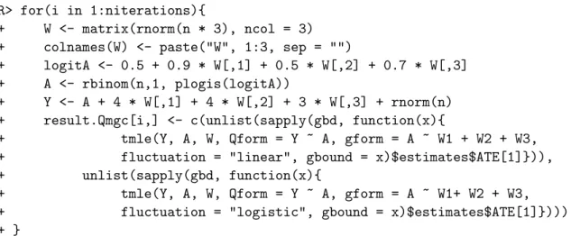
R> for(i in 1:niterations){
+ W <- matrix(rnorm(n * 3), ncol = 3)
+ colnames(W) <- paste("W", 1:3, sep = "")
+ logitA <- 0.5 + 0.9 * W[,1] + 0.5 * W[,2] + 0.7 * W[,3]
+ A <- rbinom(n,1, plogis(logitA))
+ Y <- A + 4 * W[,1] + 4 * W[,2] + 3 * W[,3] + rnorm(n)
+ result.Qmgc[i,] <- c(unlist(sapply(gbd, function(x){
+ tmle(Y, A, W, Qform = Y ~ A, gform = A ~ W1 + W2 + W3,
+ fluctuation = "linear", gbound = x)$estimates$ATE[1]})),
+ unlist(sapply(gbd, function(x){
+ tmle(Y, A, W, Qform = Y ~ A, gform = A ~ W1+ W2 + W3,
+ fluctuation = "logistic", gbound = x)$estimates$ATE[1]})))
+ }
Results in table 1 indicate that the bias of estimates arising from the logistic fluctuation is robust with respect to the choice of bound on gn, until the bias introduced by bounding
at (0.1, 0.9) begins to make a sizable contribution to the MSE. For this reason, respecting bounds by fluctuation the estimate on the logit scale is strongly recommended. The default bound for g is set to (0.025,0.975), but that guideline is flexible, and the effect on the bias and variance of the estimate depends on the data, e.g. if all values fall between (0.025,0.975), then setting bounds closer to (0,1) will have no effect at all.
Linear Logistic
gn bounds Bias Var MSE Bias Var MSE
(0, 1) −0.52 0.96 1.24 −0.03 0.11 0.11 (0.01, 0.99) −0.40 0.56 0.72 −0.03 0.11 0.11 (0.025, 0.975) −0.21 0.23 0.28 −0.03 0.09 0.09 (0.05, 0.95) 0.03 0.07 0.07 0.07 0.05 0.06 (0.1, 0.9) 0.41 0.07 0.24 0.41 0.07 0.24
Table 1: A comparison of the effect of boundinggn using a logistic or linear fluctuation in a
sparse data setting.
3.5. Controlled direct effect estimation example
The first stage of the modified TMLE procedure for CDE estimates ¯Q0(Z, A, W). All esti-mation options remain available to the user: user-specified values, user-specified parametric model, super learning, cross-validated super learning. Optional user supplied values must be specified at each level ofZ for each subject: theQargument is used to pass in ann×2 matrix of user-determined values for ¯Q0n(Z = 0, A, W). The Q.Z1 argument is used to pass in an
n×2 matrix of user-determined values for ¯Q0n(Z = 1, A, W).
In the second stageQ0n(Z, A, W) is fluctuated separately forZ = 0 and Z= 1. This requires estimation of an additional nuisance parameter,g∆=P(∆ = 1|Z =z, A=a, W)). ThepZ1 argument allows the user to pass in an n×2 matrix of conditional probabilities P(Z = 1 |
A = 0, W),P(Z = 1 | A = 1, W). Alternatively, a valid regression formula can be supplied via theg.Zform argument.
The following example illustrates CDE estimation in conjunction with missingness in the outcome. A sample of size 1000 is generated, with approximately 25% of outcomes missing.
R> n <- 1000
R> W <- matrix(rnorm(n*3), ncol = 3)
R> colnames(W) <- paste("W", 1:3, sep = "")
R> A <- rbinom(n,1, plogis(0.6*W[,1] + 0.4*W[,2] + 0.5*W[,3])) R> Z <- rbinom(n,1, plogis(0.5 + A))
R> Y <- A + A*Z+ 0.2*W[,1] + 0.1*W[,2] + 0.2*W[,3]^2 + rnorm(n) R> Delta <- rbinom(n,1, plogis(Z + A))
R> pDelta1 <- cbind(rep(plogis(0), n), rep(plogis(1), n),
+ rep(plogis(1), n), rep(plogis(2), n))
R> colnames(pDelta1) <- c("Z0A0", "Z0A1", "Z1A0", "Z1A1") R> Y[Delta == 0] <- NA
The regression formula for estimation of ¯Q0is deliberately misspecified in the next call totmle. Super learning is used to estimate the gA factor of the likelihood, but the specified library
contains only one algorithm,SL.glm, which performs a main terms regression of the outcome on all available covariates. Estimates ofgZ and g∆ are passed in to the function. Parameter estimates are reported at each level ofZ. The true parameter values areψAT E0
Z0 = 1, ψ
AT E
0Z1 = 2. R> result.Z.missing <- tmle(Y, A, W, Z, Delta = Delta, pDelta1= pDelta1,
+ Qform = Y ~ 1, g.SL.library = "SL.glm")
R> result.Z.missing Controlled Direct Effect
Z = 0 ---Additive Effect Parameter Estimate: 1.1094 Estimated Variance: 0.034713 p-value: 2.6122e-09 95% Conf Interval: (0.74419, 1.4745) Z = 1 ---Additive Effect Parameter Estimate: 1.9056 Estimated Variance: 0.011937 p-value: <2e-16 95% Conf Interval: (1.6914, 2.1197)
3.6. Marginal structural model example
All of the parameters discussed thus far have been estimated by calling the tmle func-tion. tmleMSM is a second function included in the package that can be used to estimate the parameter of a user-specified MSM for binary treatment effects. This function has many arguments in common with thetmlefunction, including(Y, A, W, Delta, Q, Qform, Qbounds, Q.SL.library, cvQinit, gform, pDelta1, g.Deltaform, g.SL.library, family, fluctuation, alpha, id, verbose). The user must also specify the marginal
structural model via theMSMargument. The same flexibility for estimating each factor of the likelihood discussed above is available: user-supplied values, user-supplied regression models, and user-specified prediction algorithm libraries for data-adaptive super learning. Additional optional arguments are available:
• V: covariates that can be used used to define strata within which to carry out the analysis
• T: time stamp for repeated measures data
• v: optional value defining the stratum of interest (V =v)
• hAV: optional numerator for constructing stabilized weights
• hAVform: optional regression formula for estimating h(A,V) as a regression of A on (V, T)
• ub: an upper bound on the weight one observation may contribute to the estimation procedure (default value is 40)
• inference: A flag controlling whether the variance-covariance matrix is constructed. The default value is TRUE, but setting inference = FALSE speeds up the execution time, and is recommended when bootstrapping.
The function calculates and returns the parameter estimates, the variance-covariance matrix, standard errors, pvalues, and 95% confidence intervals. The predicted values for the initial and targeted estimated counterfactual outcomes Qinit and Qstar are returned, along with estimated treatment assignment and missingness probabilities, g, g_Delta, and estimated values of h(A,V), along with details of the estimation procedure. These values may be used as input to subsequent calls to the tmle or tmleMSM functions. The estimated fluctuation parameter and parameter estimates based on the untargeted initialQ are also returned, to give the user some insight into how much initial estimates differ from targeted estimates, and thus the impact of applying TMLE.
Comparison of Estimators
Marginal structural models are typically fitted using inverse probability weighting (Robins 2000a; Hernan et al. 2000b; Y. Xiao 2010). We carried out a simulation study designed to demonstrate an application of TMLE and IPTW to estimating the parameter of an MSM under two different data generating distributions. The data generation scheme is taken from a paper titled Why Prefer Double Robust Estimators? (Neugebauer and van der Laan 2005), that discusses the use of inverse probability of treatment weighting (IPTW) and double robust augmented IPTW (AIPTW) estimators. One of the instructive lessons from that paper is that under near-positivity violations leading to large inverse probability weights, a double robust estimator can out-perform IPTW even when the propensity score model and the MSM are correctly specified. Since that paper pre-dates the introduction of TMLE, TMLE was not previously included in the comparison.
The observed data structure is given by O = (W, A, Y). W and Y are continuous random variables that are functions of an unobserved covariate, U, that does not confound the effect
of treatment on the outcome. Treatment assignment is a function of W. We are interested in estimating the two-dimensional parameter β of an MSM given by Y = β0+β1A, where the true value ofβ = (β0, β1) = (2,−5). Three estimators were applied to this problem, the
tmleMSMfunction, the IPTW estimator using unstabilized weights, wti= 1/gn(Ai|Wi and a
second IPTW estimator using stabilized weights,wti,stab =
1 n Pn i=1(A=Ai) /gn(Ai|Wi).
Two treatment assignment mechanisms were defined that differ in the strength of the associ-ation between A and W.
g1 = P(A= 1|W) =expit(0.1 + 0.25W)
g2 = P(A= 1|W) =expit(1 + 1.5W)
The empirical probability of receiving treatment according to mechanism g1 ranges between approximately 0.16 and 0.88, corresponding to inverse weights of 1.14 and 6.25. These val-ues indicate that except possibly at extremely small sample size, no observation would re-ceive enough weight to completely dominate the analysis. In contrast, treatment assignment probabilities based on mechanism g2 range between 6×10⁻⁵ and 0.999995. We call this a near-positivity violation, and it poses a challenging estimation scenario.
Notice that under this specification of the MSM, the coefficient β1 is equivalent to the ATE parameter estimated by the tmle function. We would expect the estimate of β1 obtained using the tmleMSM function to be equal to the estimate of the ATE parameter returned by the tmle function (allowing for a certain imprecision due to the differences in the way the calculations are carried out). The simulation results bear this out. We also estimate the ATE parameter using an alternative double-robust estimator, the augmented IPTW estimator (AIPTW) introduced in Robins and Rotnitzky (1992). The AIPTW estimator is defined as,
ψAIP T Wn = 1 n n X i=1 [I(Ai = 1)−I(Ai= 0)] gn(Ai |Wi) (Yi−Q¯0n(Ai, Wi)) + 1 n n X i=1 ( ¯Q0n(1, Wi)−Q¯0n(0, Wi)).
R code that defines a function to calculate AIPTW estimates of the ATE parameter given datasetd, outcome regression modelQform, and estimated treatment assignment probabilities,
g1W is shown next.
R> calc_aipw <- function(d, Qform, g1W) { R> Q <- glm(Qform, data = d)
R> QAW.pred <- predict(Q)
R> Q1W.pred <- predict(Q, newdata = data.frame(d[,-2], A = 1)) R> Q0W.pred <- predict(Q, newdata = data.frame(d[,-2], A = 0)) R> h <- d$A/g1W - (1- d$A)/(1 - g1W)
R> return(psi = mean(h*(d$Y - QAW.pred) + Q1W.pred - Q0W.pred))
R> }
The next code chunk runs the Monte Carlo simulation study. The outside loop corresponds to the two treatment assignment mechanisms. Within the inner loop a dataset is generated at each iteration and subsequently analyzed. Models for the MSM and the conditional distribu-tion of the treatment assignment are correctly specified, and the same (unbounded) predicted
treatment assignment probabilities are used by each estimator. The specification of the model forQ is slightly misspecified for TMLE and AIPTW estimators, by omitting the unobserved covariate,U, but this omission does not bias the estimate of the ATE parameter.
R> set.seed(10) R> n <- 500 R> niter <- 500 R> a <- c(.1, 1) R> b <- c(.25,1.5)
R> est.beta0 <- array(NA, dim = c(2, niter, 3), + dimnames = list(c("g1", "g2"), NULL, + c("IPW", "IPW stabilized", "TMLE.MSM"))) R> est.ATE <- array(NA, dim = c(2, niter, 5), + dimnames = list(c("g1", "g2"), NULL,
+ c("IPW", "IPW stabilized", "TMLE.MSM", "TMLE", "AIPW"))) R> for (i in 1:2){
R> for (j in 1:niter){
R> U <- runif(n, -10, 10) R> W <- U/3 + rnorm(n) R> logitA <- a[i] + b[i]*W
R> A <- rbinom(n, 1, plogis(logitA))
R> Y <- 2 + 4 * U - 5 * A + rnorm(n)
R> g <- glm(A ~ W, family = "binomial") R> g1W <- predict(g, type = "response")
R> wt <- A/g1W + (1 - A)/(1 - g1W)
R> wt.stab <- (A * mean(A) + (1 - A) * (1 - mean(A))) * wt
R> ipw.msm <- coef(glm(Y ~ A, weights = wt))
R> ipw.stab.msm <- coef(glm(Y ~ A, weights = wt.stab))
R> res.tmleMSM <- tmleMSM(Y, A, as.matrix(W), V = rep(1, n), MSM = "A",
+ Qform = "Y ~ A", g1W = g1W, ub = Inf)
R> res.tmle <- tmle(Y, A, as.matrix(W), Qform ="Y ~ A", g1W = g1W,
+ gbound = c(0,1))
R> aipw <- calc_aipw(data.frame(Y, A, W), Qform = "Y ~ A", g1W = g1W)
R> est.beta0[i,j,] <- c(ipw.msm[1], ipw.stab.msm[1], res.tmleMSM$psi[1])
R> est.ATE[i,j,] <- c(ipw.msm[2], ipw.stab.msm[2], res.tmleMSM$psi[2],
+ res.tmle$estimates$ATE$psi, aipw)
R> }}
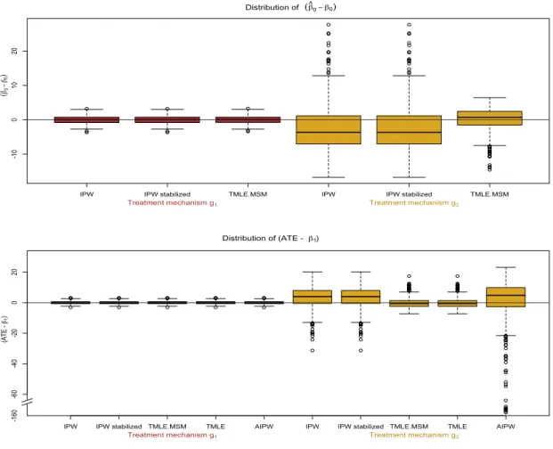
Results displayed in Figure 1 and listed in Table 2 indicate that all estimators perform well under treatment assignment mechanism g1. When the more extreme treatment assignment mechanism is used to generate the data (g2), performance of the IPTW estimators and AIPTW degrades significantly, while both TMLEs exhibit only modest increases in bias and variance.
TMLE is a substitution estimator that ensures global bounds of the statistical model are respected, thereby constraining the bias and variance. Both AIPTW and TMLE solve the same estimating equation and are asymptotically equivalent estimators of the ATE parameter. However, as illustrated by the plots in the figure and the results reported in Table2, depending
IPW IPW stabilized TMLE.MSM IPW IPW stabilized TMLE.MSM -10 0 10 20 Distribution of (β^0−β0)
Treatment mechanismg1 Treatment mechanismg2
(
β
^−0 β0
)
IPW IPW stabilized TMLE.MSM TMLE AIPW IPW IPW stabilized TMLE.MSM TMLE AIPW
-60 -40 -20 0 20 -160 Distribution of (ATE - β1)
Treatment mechanismg1 Treatment mechanismg2
(ATE -
β1
)
Figure 1: Distribution of parameter estimates minus the true parameter value under two different treatment assignment mechanisms, no positivity violations (g1, left), and practical
positivity violations(g2, right)
on the characteristics of the underlying data distribution the difference in their finite sample performance can be striking. An in-depth discussion of the relative performance of TMLE in comparison with other double robust estimators discussed in the literature can be found in
Porter et al. (2011).
4. FEV data analysis
TMLE was applied to assess the marginal effect of smoking on forced expiratory volume (FEV) using data originally introduced inRosner(1999b) and discussed inKahn(2005). The data consists of 654 observations with five variables recorded for each subject: age (years),
fev(liters),ht(height in inches),sex(0=female, 1=male),smoke(0=non smoker, 1=smoker) (Rosner 1999a). FEV is a measure of pulmonary function that is related to body size and lung capacity. Thus, the relationship between smoking and FEV is likely to be confounded by age and sex, both of which influence FEV and are associated with smoking status. Though height does not have an obvious link to smoking behavior accounting for covariates predictive
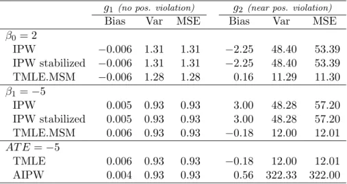
Table 2: Estimator comparison,n= 500
g1 (no pos. violation) g2 (near pos. violation) Bias Var MSE Bias Var MSE
β0= 2 IPW −0.006 1.31 1.31 −2.25 48.40 53.39 IPW stabilized −0.006 1.31 1.31 −2.25 48.40 53.39 TMLE.MSM −0.006 1.28 1.28 0.16 11.29 11.30 β1=−5 IPW 0.005 0.93 0.93 3.00 48.28 57.20 IPW stabilized 0.005 0.93 0.93 3.00 48.28 57.20 TMLE.MSM 0.006 0.93 0.93 −0.18 12.00 12.01 AT E =−5 TMLE 0.006 0.93 0.93 −0.18 12.00 12.01 AIPW 0.004 0.93 0.93 0.56 322.33 322.00
of the outcome can improve efficiency, so we include it in the analysis. The data are from an observational study of children 3 -19 years old. No children younger than nine years old smoked cigarettes. Therefore, any attempt to estimate a marginal effect of smoking on FEV adjusted for age incurs a theoretical ETA violation due to a complete lack of support in the data. For this reason we restrict the analysis to the subset of data containing n = 439 observations on subjects ages 9 - 19.
The observed data consists of n i.i.d. copies of O = (W, A, Y) ∼ P0, where W = (age, ht, sex),A is an indicator of smoking status, andY is a continuous measure of FEV. The outcome of interest is the marginal additive effect of smoking on FEV, defined asEW[E(Y | A= 1, W)−E(Y |A= 0, W)]. If the true regression ofY on A and W were a main terms linear regression, this parameter would correspond to the coefficient in front of the treatment term. However, there is no reason to believe that is the case, and an estimate of the treatment effect based on this misspecified model for ¯Q is likely to be biased. The double-robustness property of TMLE tells us that even given a misspecified ¯Q0n, the targeting step can reduce this bias, given a consistent estimate of the treatment mechanism. In the next example we deliberately supply a main terms model for ¯Q that we assume is misspecified, and use super learning to estimategA(1|W). The algorithms included in the super learner library are:
• SL.glm main terms logistic regression ofA on W (Team 2011).
• SL.stepstepwise forward and backward model selection using AIC criterion, restricted to second order polynomials (Team 2011).
• SL.DSA.2 DSA algorithm searching over second order polynomials, substitution and addition moves enabled(Neugebauer and Bullard 2010).
• SL.loesslocal fitting of a polynomial response surface (span = 0.75) (Team 2011).
• SL.caretrandom forest, with data-adaptively selected value formtryparameter (Kuhn, Wing, Weston, Williams, Keefer, and Engelhardt 2010).
• SL.bart a classifier based on a Bayesian sum-of-trees model (ntree = 300) (Chipman and McCulloch 2010).
• SL.knn, SL.knn20, SL.knn40, SL.knn60 k-nearest neighbor algorithm, with neigh-borhood size, k, set to 10, 20 ,40 ,60 (Venables and Ripley 2002).
R> data(fev)
R> fev <- fev[fev$age >= 9,]
R> g.SL.library <- c("SL.glm", "SL.step", "SL.DSA.2","SL.loess", "SL.caret", + "SL.bart", "SL.knn", "SL.knn20", "SL.knn40", "SL.knn60") R> smoke.Qmis <- tmle(Y = fev$fev, A = fev$smoke, W = fev[ ,c(1, 3, 4)],
+ Qform = Y ~ ., g.SL.library = g.SL.library)
R> smoke.Qmis Additive Effect Parameter Estimate: -0.099653 Estimated Variance: 0.0045071 p-value: 0.13771 95% Conf Interval: (-0.23124, 0.031932)
The parameter estimate after targeting is 1/nPn i=1Q¯
∗
n(1, Wi)−Q¯n∗(0, Wi) = −0.10. Users
are often curious about how targeting affects the parameter estimate. The function returns initial (untargeted) predicted values, ¯Q0n(0, W),Q¯0n(1, W). This allows the user to calculate a parameter estimate of -0.16 based on the initial estimate of ¯Q0 as follows:
R> EY0 <- mean(smoke.Qmis$Qinit$Q[,"Q0W"]) R> EY1 <- mean(smoke.Qmis$Qinit$Q[,"Q1W"]) R> EY1 - EY0
[1] -0.1574331
Recall that TMLE is asymptotically efficient when both ¯Q0 andg0 are estimated consistently. In the next example, instead of starting with a deliberately misspecified model for ¯Q0, super learning is applied to estimate ¯Q0. The prediction algorithm library includes all the algorithms specified for the estimation ofg that do not require a binary outcome (everything except the
k-nearest neighbor algorithms), and also a linear regression of Y on A and W that includes main terms and all interactions of A and W. We begin by defining a new super learner wrapper function,SL.glm.int:
R> SL.glm.int <- function(Y.temp, X.temp, newX.temp, family, ...){ + Aint <- paste("A", colnames(X.temp)[-c(1, 2)], sep = "*") + form <- paste("Y.temp ~ Z + ", paste(Aint, collapse = "+"))
+ fit.glm <- glm(form, data = data.frame(Y.temp, X.temp), family = family)
+ out <- predict(fit.glm, newdata = newX.temp, type = "response")
+ fit <- list(object = fit.glm)
+ foo <- list(out = out, fit = fit)
+ class(foo$fit) <- c("SL.glm.int")
+ return(foo)
+ }
R> Q.SL.library <- c("SL.glm", "SL.glm.int", "SL.DSA.2", + "SL.loess", "SL.caret", "SL.bart")