Statistical Scalability Analysis of Communication
Operations in Distributed Applications
Jeffrey S. Vetter
Michael O. McCracken
Center for Applied Scientific Computing Lawrence Livermore National Laboratory
Livermore, California, USA 94551 {vetter3,mccracken6}@llnl.gov
ABSTRACT
Current trends in high performance computing suggest that users will soon have widespread access to clusters of multiprocessors with hundreds, if not thousands, of processors. This unprecedented degree of parallelism will undoubtedly expose scalability limitations in existing applications, where scalability is the ability of a parallel algorithm on a parallel architecture to effectively utilize an increasing number of processors. Users will need precise and automated techniques for detecting the cause of limited scalability. This paper addresses this dilemma. First, we argue that users face numerous challenges in understanding application scalability: managing substantial amounts of experiment data, extracting useful trends from this data, and reconciling performance information with their application’s design. Second, we propose a solution to automate this data analysis problem by applying fundamental statistical techniques to scalability experiment data. Finally, we evaluate our operational prototype on several applications, and show that statistical techniques offer an effective strategy for assessing application scalability. In particular, we find that non-parametric correlation of the number of tasks to the ratio of the time for communication operations to overall communication time provides a reliable measure for identifying communication operations that scale poorly.
1 INTRODUCTION
Current trends in high performance computing suggest that users will be running their applications on scalable clusters of multiprocessors with hundreds, if not thousands, of processors in the near future [3, 15]. This unprecedented availability of computing resources motivates the need for precise and meaningful scalability analysis of these applications. By
scalability, we mean the ability of a parallel algorithm on a parallel architecture to effectively utilize an increasing number of processors [6, 7, 13]. Undoubtedly, this new, high degree of concurrency will expose scalability limitations of applications that, at lower levels of concurrency, might have been shrouded by other application or system characteristics. Furthermore, perpetual improvements in single node performance will continue revealing the scalability limitations of communication operations in their distributed applications.
Although metrics like execution time, speedup, and efficiency [14] help quantify scalability on an abstract level, users need precise information about poorly scaling communication operations in their application. In addition, for any analysis to help users understand their application’s scalability, the technology should be able to explain scalability phenomena in terms of decisions a user makes while designing their application.
To this end, we propose an automated technique that uses familiar statistical techniques to direct a user's attention on poorly scaling communication operations in their application. Our method digests the results of multiple application experiments and suggests communication operations whose growth has a positive correlation with the number of tasks. We empirically evaluate the usefulness of these techniques on nine applications with both fixed and scaled problem sizes. Our results show that, in every case, our method quickly identifies the communication operations that grow to dominate the application's execution time during highly parallel experiments. More importantly, our technique selects operations that a user might not normally locate when using simpler methods.
1.1 Background
The analysis of scalability is not a new concept [6, 14]. Yet many users find scalability analysis of their applications difficult, time-consuming, and inconclusive. Despite the fact that investigators have proposed numerous metrics, such as speedup, scaled speedup, efficiency, and iso-efficiency, these metrics provide only an abstract and broad view of application scalability behavior. They do not provide specific evidence that allows users to understand and optimize their applications. Worse, the experimental process of measuring application scalability, in practice, can generate an intractable amount of data. This fact alone can hinder the effort, because users are basically inundated with lots of uninteresting, redundant data.
Aside from this work, various teams have proposed scalable visualization techniques for understanding performance data [5, 10, 21]; however, many of these techniques have not been
extended to help users understand application scalability. Essentially, this previous work has focused on helping users understand the performance data of one application experiment, whereas scalability analysis forces users to integrate performance data from many experiments.
The goal of this work, in contrast, is to develop techniques that promptly and reliably focus a user’s attention on the communication operations of their application that limit scalability. With this guidance, a user can easily locate scalability problems and modify their application, if necessary. Our work is empirically driven and directly relevant to existing applications. In fact, our analysis focuses on the Message Passing Interface (MPI) [9, 20] because it serves as an important foundation for a large group of high performance applications and communication scalability will become an increasingly important problem as the size of computing systems continues to increase [4, 18, 23].
1.2 Paper
Organization
The remainder of this paper discusses these issues in more detail. In Section 2, we motivate scalability analysis with a case study and observe that users need automated techniques for scalability analysis. Following this, in Section 3, we introduce our approach to analyzing scalability data with statistical techniques. Then, in Section 4, we evaluate these techniques on numerous MPI applications. Finally, Section 5 concludes the paper with a summary and some interesting research directions.
2
MOTIVATING EXAMPLE
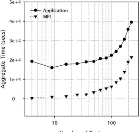
To motivate the demands of scalability analysis, we consider a case study of NAS BT [1]. (Section 4 provides complete details of the experimental evaluation.) The goal of this example is to outline the process of manual scalability analysis and to argue for an automated technique. 1XPEHURI7DVNV $ JJ UH JD WH 7 LP H V HF V H H H H H $SSOLFDWLRQ 03,
Figure 1: NAS BT Communication Time.
As a first step in analyzing the scalability of BT, we look first at the aggregate runtime of BT from 4 tasks up to 225 tasks as illustrated in Figure 1. More specifically, we divide the time in each task into communication, Tcomm, and computation, Tcomp (or
MPI in Figure 1). We capture these values empirically. Each task i has a Ti,comm, and Ti,comp that together create Ti,app, the execution
time of task i. We define Tagg as the processor-time summation
across all tasks:
∑
∑
= = + = = N i comp i comm i N i i agg T T T T 1 , , 1 ) (Likewise, we define the aggregate time for communication across all tasks as Tagg,comm:
∑
= = N i comm i comm agg T T 1 , ,Noting that we use the fixed problem size of Class B for this experiment, Figure 1 shows the breakdown of communication time as part of the aggregate application runtime for each experiment size. This analysis quickly illustrates that, for this problem size, BT effectively uses an increasing number of processors up to 81. However, at this point, BT’s communication time forces the application time higher.
Noticeably, some portion of the communication in BT is increasing; however, this resolution remains too coarse. It is unclear whether all communication operations degrade evenly, or whether one or two communication operations are causing the dramatic increase in communication time.
Number of Tasks 10 100 Ag gre g a te T im e (m ill is e c s ) 0.0 2.0e+6 4.0e+6 6.0e+6 8.0e+6 1.0e+7 1.2e+7 1.4e+7 1.6e+7 Allreduce Barrier Comm_dup Comm_rank Comm_size Comm_split Irecv Isend Reduce Wait Waitall
Figure 2: NAS BT Communication Time by Type.
As a next step, we decompose the communication time by operation (e.g., barrier, reduction, send). Many MPI performance analysis tools capture data by the type of MPI call and they do not distinguish among different call sites to the same MPI library routine. Restated, we now have
∑
=allops j j i comm i T T, ,where Ti,op provides the total time that task i spent in the op type
of communication operation. Figure 2 shows the breakdown of communication operations by type for BT. Viewed in this light, we can focus our scalability analysis on one type of communication operation in BT: Wait, Barrier, Waitall, and
Comm_split. Up to 81 tasks, Tagg,wait remains the largest
component, but relatively constant; yet beyond 81 tasks, Tagg,wait
dominates the communication time. Also, Barrier, Waitall, and
Comm_split emerge noticeably from the group as the number of
tasks increase.
Realistically, however, applications call these operations from multiple call sites. So, as a final step, we split Tagg,wait into
∑
=allcallsites j j wait i wait i T T, , , ,we find that not all Wait operations perform similarly as Figure 3 indicates for several select call sites. Indeed, two of the four Waits scale admirably while the other two waits, at x_solve.f:71 and
y_solve.f:70, perform much worse.
1XPEHURI7DVNV $ JJ UH JD WH 7 LP H P LOO LV HF V H H H H H :DLW[BVROYHI &RPPBVSOLWVHWXSI %DUULHUEWI :DLW\BVROYHI :DLW]BVROYHI :DLW\BVROYHI
Figure 3: NAS BT communication time for select call sites.
In fact, this decomposition of the communication time by call site illustrates several interesting characteristics about BT. First, many of the data points are quite noisy. Take, for instance, the
Comm_split data in Figure 3. These sample points oscillate wildly
even though the communication time increases steadily in Figure 1. Our experience indicates that this noise is commonplace, especially on large, production computing systems. Second, the shape of the curves in Figure 3 is strikingly similar to the communication time in Figure 1. All the call sites are relatively flat up to 81 tasks.
In any case, given this information, a user could begin a detailed investigation into why these operations scale poorly, especially when considering that calls to the same communication operation perform differently. The reason for poor scaling could have a number of causes including poor load balance and algorithm design. Also, using this evidence from all call sites, a user could compare calls to the same communication routine and rule out implementation problems for all but the most pathological cases.
2.1 Observations
This example illustrates the basic problems encountered by any user when they try to analyze application scalability. First, although the analysis provides some information about scalability, it only provides precise evidence once the user has manually searched through the data to harvest the offensive communication operations. We selected the BT example because it was illustrative; other real world applications will force users to manage similar data for hundreds of MPI call sites across thousands of tasks.
Consider that for one experiment, with P processors executing n communication operations, the analysis can produce data at the rate of approximately n × P events at any time t. In addition, scalability analysis requires data from E experiments, leading to at least n × P × E data points. Taken together, these factors can, over a very short period of time, overwhelm most users.
Furthermore, any analysis must account for statistical variations in the experiments as illustrated in our BT example. In this analysis, we ran four experiments at every size of N, and then selected the experiment with the smallest running time as the representative for that experiment group. Alternatively, a quantitative analysis should use this additional data to strengthen or weaken the conclusions of the experiments.
3
STATISTICAL SCALABILITY
ANALYSIS
Given the issues of manual scalability analysis as exposed in Section 2, we propose an alternative solution that relies on statistical analysis [11, 16] to extract meaningful relationships from the data. With our solution, users can easily distill the results of their scalability experiments, automatically revealing communication operations that scale poorly.
Scalability Analysis Experiments
256 64
128
Clean and Merge Comm Data By Callsite Calculate Ratios Rank Transformation Calculate Correlation Coefficient Select Poorly Scaling Ops
Figure 4: Process for statistical scalability analysis.
Figure 4 illustrates our process for statistical scalability analysis. Our process is composed of two stages. First, the user performance multiple scalability experiments varying the number of tasks, and possibly, the problem size. During each experiment, we record specific timing information about call sites for all communication operations. The user can perform multiple experiments at each configuration; and, in fact, we encourage this. The next step in our process merges all of the scalability experiment files and then harvests timing information about each call site. With this information in hand, we calculate the ratio of the aggregate time in each call site to the aggregate communication time. We, then, rank transform both this ratio and the number of tasks for each experiment. Finally, our process calculates the correlation between the ranked ratio and the ranked number of tasks.
As we will show in Section 4, we find that this non-parametric (or rank) correlation of aggregate times provides an accurate and stable predictor for identifying communication operations that scale poorly.
3.1 Performance Data Management
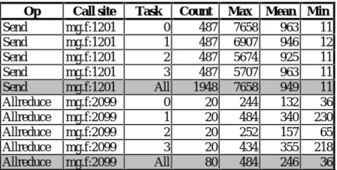
We organize our data to reflect the stages of scalability analysis presented in Section 2. Our analysis assumes that for all call sites across all tasks in the application, we have the count, cumulative time, minimum time, and maximum time. Table 1 shows an example of this performance data from MG.Op Call site Task Count Max Mean Min Send mg.f:1201 0 487 7658 963 11 Send mg.f:1201 1 487 6907 946 12 Send mg.f:1201 2 487 5674 925 11 Send mg.f:1201 3 487 5707 963 11 Send mg.f:1201 All 1948 7658 949 11 Allreduce mg.f:2099 0 20 244 132 36 Allreduce mg.f:2099 1 20 484 340 230 Allreduce mg.f:2099 2 20 252 157 65 Allreduce mg.f:2099 3 20 434 355 218 Allreduce mg.f:2099 All 80 484 246 36
Table 1: Call site data for one experiment on NAS MG.
We have constructed a software tool, using the MPI profiling layer [9], to provide straightforward access to this type of data. In addition, we capture the runtime of each task, from start to finish. With this information, we can do all of the analysis presented in Section 2 and we can compute derived values, such as speedup. For scalability analysis, we have several options for organizing the data. One alternative is to compare call site times for each task in one experiment to the same call site times in other experiments. This option has the disadvantage that, by definition, experiments have different numbers of tasks, so it does not make sense to compare call site values task-wise across experiments. As a result, we chose our second strategy for analyzing call site data: we aggregate the call site values across all tasks for each experiment and compare the aggregation with similar aggregations for other experiments. Table 2 shows aggregate call site data for three BT experiments. NUMBER OF TASKS CALL SITE 9 16 25 Barrier:bt.f:193 11.7 26.56 58.75 Waitall:copy_faces.f:207 137440.8 232704 358045 Wait:y_solve.f:70 122610 24240.6 44461.2 Comm_split:setup_mpi.f:50 23.04 39.84 81.5
Table 2: Aggregate call site data for three BT experiments.
This choice has numerous implications. First, by aggregating the time, we suppress subtle differences across tasks and possibly, squander information that could pinpoint a load imbalance. Second, this aggregation has different results for scaled or fixed problem sizes. However, we compensate for this difference by using a ratio rather than a raw time in our final analysis.
3.2 Correlation Coefficient
For our data analysis, we turn to the correlation coefficient for two reasons. First, correlation is a relatively simple and well-understood technique, and the process of relating the results of more complex statistical measures to source code can be challenging. Second, other techniques, such as curve fitting, are often difficult to calculate for non-linear functions or noisy sample data, as is regularly the case with performance data. The sample correlation coefficient, r, measures the linear association between two variables and does not depend on the units of measurements. The standard equation for the linear correlation coefficient is
∑
∑
∑
− − − − = i i i i i i i y y x x y y x x r 2 2 ) ( ) ( ) )( ( .The value of r must be between -1 and +1. Quantitatively, r measures the strength of the linear association between two variables. If r is near 0, it implies no association between the variables, or that they are uncorrelated. Otherwise, the sign of r specifies the direction of the association. If r is negative, it implies an inclination for one value in the pair to be larger than its average when the other is smaller than its average. If r is positive, it suggests a tendency for one value of the pair to be large when the other value is large and also for both values to be small together. Disappointingly, however, the linear correlation coefficient suffers several limitations. First, it assumes that the underlying distributions are normal. Second, nonlinear associations can exist that are not revealed by the linear correlation coefficient. Third, linear correlation can be very sensitive to outliers, showing an association between variables when it does not exist. Finally, correlation does not imply causality in the association. We address these limitations by using rank transformation and by applying the correlation computation in a very restricted way.
In addition to rank transformation, we can argue that, in our context, our data does not have nonlinear relationships and that it does imply causality. Our argument relies on the fact that, as we have designed it, the application’s total communication time is the sum of all the application’s communications operations. An increase in any operation’s time directly increases the total communication time. So, it is a linear and casual relationship by design.
Another important point is that correlation can accept any number of scalability experiments, including experiments with identical configurations. This only improves the analysis either by strengthening or weakening the relationship between individual communication operations and the total communication time. That is, if two identically configured experiments have the same communication times yet produce drastically different measurements for one call site, then any conclusion about that call site must be interpreted carefully.
3.3 Rank Transformation
Because we are concerned about the normality assumption of the linear correlation technique and the effect of outliers in our measurements, we perform non-parametric or rank correlation [11, 16] on our data. Rank transformation is the process of replacing the actual observations by their ranks. Assume that we are given N pairs of measurements: X, Y. The key notion of non-parametric correlation is to replace the value of each x by the value of its rank among all other xs in the sample: R, S. The transformed list will be drawn from a uniform distribution function from the integers between 1 and N, inclusive. The values for Y are transformed in the same way. When some of the values are identical, we assign these values the midrank for their range: the mean of the ranks of that these values would have occupied if their values were different. In particular, we use the Spearman rank correlation coefficient:
∑
∑
∑
− − − − = i i i i i i i s S S R R S S R R r 2 2 ( ) ) ( ) )( ( .We prefer the rank transformed correlation because it is less likely to be distorted by non-normality and unusual observations.
1XPEHURI7DVNV5DQN 5D QN R I 5D WL R RI & DO OV LW H 7L P H WR 0 3, 7 LP H Wait:x_solve.f:71 Comm_split:setup_mpi.f:50 Barrier:bt.f:193 Wait:y_solve.f:70 Wait:z_solve.f:95 Wait:y_solve.f:97
Figure 5: Example rank scatterplot of BT call sites.
Figure 5 illustrates a scatterplot of several BT call sites after the ranking. Associations clearly emerge between the number of tasks and several call sites in this figure. The first four call sites,
Wait:x_solve.f:71, Comm_split:setup_mpi.f:50, Barrier:bt.f:193, and
Wait:y_solve.f:70, are positively correlated with the number of
tasks, while Wait:z_solve.f:95 and Wait:y_solve.f:97 are negatively correlated.
4 EXPERIMENTAL
EVALUATION
To explore our hypothesis of using rank correlation to analyze scalability, we have constructed an operational prototype for MPI applications. With this prototype, we empirically evaluated nine applications from the NAS Parallel suite and the ASCI Compact Benchmarks.
4.1 Experiment Overview
To capture information about the communication operations within these MPI applications, we extract information about each MPI call during application execution, as discussed in Section 3. Unlike trace-based performance analysis tools [8, 17, 19], our lightweight profiler captures only fundamental performance data about MPI call sites: number of times called and cumulative time spent in the call. In fact, Table 1 shows profiler output for one NAS MG experiment. Call site is location of the MPI function in the user’s the source code. Rank identifies each MPI task’s rank within communicator MPI_COMM_WORLD. All represents the aggregate values across all tasks for that call site. Count provides the number of times that function at that call site was called. Max,
Min, and Mean capture the maximum, minimum, and mean duration, respectively, for each call site.
We have found that this profiling technique balances the requirements of low overhead and manageable data volume with the need for information about an application’s communication.
Furthermore, the amount of data generated with this lightweight technique is invariant to the length of the application’s run time. Put another way, the amount of profiler output for an application experiment is effectively constant whether the application runs for 5 minutes or 5 days. Note that users can apply the techniques developed here to information gathered with trace files.
For these evaluations, we analyze each application from start to finish; therefore, these results contain initialization and setup phases that might not be included in strict algorithmic evaluations.
4.2 Platform
We ran our tests in the batch partition of the ASCI Blue Pacific combined technology refresh (CTR) SP at Lawrence Livermore National Laboratory. This machine is composed of 332 Mhz 604e 4-way SMP nodes, totaling 1344 CPUs. Each compute node has a peak performance of 2.656 GigaOPS. The 604e processor has one floating-point unit and one load/store unit. Its 32KB L1 cache is 4 way associative with 32 byte cache lines and L1 uses an LRU replacement scheme. The processor has a 500KB L2 cache. At the time of our tests, the batch partition had 305 nodes and the operating system was AIX 4.3.3. We compiled the various tests with the IBM XL compilers and used IBM’s MPI library in user-space mode. Each SMP node contains 1.5 GB main memory for a total of 504 GB system memory. Node to node bi-directional bandwidth is 150 Mbyte/s. Our test jobs ran on dedicated nodes, although other jobs were concurrently using the network.
4.3 Application Results
We tested six of the benchmarks from NAS Parallel Benchmark 2.3 suite [1]: BT, SP, MG, FT, LU, and CG. These NAS benchmarks are fixed-problem size; our experiments use class B problems. We also tested other applications from the ASCI Compact Benchmark suite: sPPM, Sweep3d, and SMG2000. These benchmarks scale problem sizes with the number of tasks. Table 4 outlines the experiment configurations for these applications. We performed the experiment at least three times at each configuration.
Application Scaled problem,
Problem size
Experiment range
NAS BT No, Class B 4 - 225 NAS CG No, Class B 2 - 256 NAS FT No, Class B 8 - 256 NAS LU No, Class B 4 - 256 NAS MG No, Class B 2 - 256 NAS SP No, Class B 4 - 225 SMG2000 Yes, 10x10x10 per task 2 - 1024 SPPM Yes, 1283 per task 2 - 768
Sweep3D Yes, 6x6x300 per task 2 - 512
Table 4: Applications.
Table 3 presents the rank correlation results for all the applications we studied. We limited the call sites included in the table to those call sites that exceeded a threshold of 1% for at least one of the experiments on that application. For clarity, we graph only the data points for each experiment configuration whose aggregate execution time was the minimum for that configuration.
4.3.1 NAS Parallel Benchmarks
Figure 6 shows our scaling results for the NAS benchmarks. All of the NAS benchmarks scale well, given that they are constrained by their fixed problem size. As other researchers have noted [24], these benchmarks effectively utilize an increasing number of processors up to a limit where they begin suffering from their inevitable growth in communication overhead and from their
shrinking local problem size.
The benchmark applications NAS SP and BT represent computational fluid dynamics (CFD) applications that solve systems of equations resulting from an approximately factored implicit finite-difference discretization of the Navier–Stokes equations. The SP and BT algorithms have a similar structure; each solves three sets of uncoupled systems of equations. BT solves block-tridiagonal systems of 5x5 blocks; SP solves scalar
bt.B rs mg.B rs lu.B rs
Wait:x_solve.f:71 0.93 Wait:mg.f:1315 0.89 Allreduce:l2norm.f:55 0.75 Comm_split:setup_mpi.f:50 0.90 Wait:mg.f:1542 0.70 Bcast:bcast_inputs.f:28 0.73 Barrier:bt.f:193 0.89 Barrier:mg.f:99 0.67 Send:exchange_3.f:275 0.46 Wait:y_solve.f:70 0.64 Barrier:mg.f:2089 0.62 Recv:exchange_1.f:30 0.45 Wait:y_solve.f:0 0.44 Allreduce:mg.f:1004 0.48 Send:exchange_3.f:209 0.41 Wait:z_solve.f:68 0.42 Allreduce:mg.f:2139 0.43 Send:exchange_1.f:149 0.30 Wait:x_solve.f:0 -0.06 Allreduce:mg.f:1001 0.41 Send:exchange_1.f:130 -0.01 Wait:x_solve.f:99 -0.07 Allreduce:mg.f:2099 0.41 Recv:exchange_1.f:48 -0.04 Wait:y_solve.f:69 -0.32 Allreduce:mg.f:2115 0.39 Send:exchange_1.f:166 -0.08 Wait:z_solve.f:0 -0.32 Allreduce:mg.f:2123 0.33 Send:exchange_1.f:113 -0.13 Barrier:bt.f:147 -0.44 Barrier:mg.f:233 0.09 Recv:exchange_1.f:86 -0.13 Wait:x_solve.f:70 -0.47 Reduce:mg.f:256 0.01 Send:exchange_3.f:139 -0.18 Wait:y_solve.f:98 -0.53 Bcast:mg.f:133 -0.06 Recv:exchange_1.f:68 -0.21 Wait:z_solve.f:96 -0.56 Send:mg.f:1215 -0.11 Send:exchange_3.f:73 -0.25 Wait:z_solve.f:67 -0.86 Irecv:mg.f:1160 -0.13 Wait:exchange_3.f:288 -0.44 Wait:x_solve.f:98 -0.92 Send:mg.f:1247 -0.15 Wait:exchange_3.f:222 -0.46 Waitall:copy_faces.f:207 -0.95 Send:mg.f:1233 -0.27 Wait:exchange_3.f:152 -0.83 Wait:z_solve.f:95 -0.96 Send:mg.f:1265 -0.33 Wait:exchange_3.f:86 -0.92 Wait:y_solve.f:97 -0.97 Comm_rank:mg.f:86 -0.36 Send:mg.f:1201 -0.41 cg.B rs sp.B r s Send:mg.f:1279 -0.48 Barrier:cg.f:411 0.91 Comm_split:setup_mpi.f:51 0.85 Wait:cg.f:1221 0.90 Barrier:sp.f:189 0.77 sppm r s Wait:cg.f:1275 0.90 Waitall:y_solve.f:74 0.71 Allreduce:main.f:1392 0.81 Wait:cg.f:1397 0.85 Bcast:sp.f:102 0.65 Wait:bdrys.f:1247 0.75 Wait:cg.f:1059 0.58 Allreduce:error.f:50 0.35 Wait:bdrys.f:1248 0.73 Wait:cg.f:1150 0.44 Isend:x_solve.f:335 0.18 Wait:bdrys.f:928 0.72 Irecv:cg.f:1318 0.43 Waitall:x_solve.f:81 -0.03 Wait:bdrys.f:3596 0.63 Wait:cg.f:1177 -0.23 Barrier:sp.f:143 -0.19 Wait:bdrys.f:2421 0.54 Send:cg.f:1326 -0.66 Waitall:z_solve.f:73 -0.39 Allreduce:main.f:1025 0.48 Send:cg.f:1143 -0.76 Waitall:y_solve.f:380 -0.78 Wait:bdrys.f:2422 0.46 Send:cg.f:1354 -0.76 Waitall:z_solve.f:377 -0.91 Wait:bdrys.f:2953 0.45 Send:cg.f:1170 -0.79 Waitall:x_solve.f:388 -0.92 Wait:bdrys.f:2954 0.34
Waitall:copy_faces.f:208 -0.94 Wait:bdrys.f:2102 -0.03 smg2000 rs Wait:bdrys.f:1780 -0.24 Allreduce:timing.c:419 0.93
ft.B rs Wait:bdrys.f:3595 -0.24 Allreduce:struinprod.c:107 0.92 Bcast:ft.f:443 0.87 Wait:bdrys.f:927 -0.28 Waitall:coarsen.c:542 0.83 Comm_split:ft.f:506 0.86 Wait:bdrys.f:1779 -0.33 Waitall:coarsen.c:491 0.80 Barrier:ft.f:118 -0.41 Wait:bdrys.f:3276 -0.50 Barrier:smg2000.c:227 0.71 Alltoall:ft.f:1283 -0.91 Wait:bdrys.f:3275 -0.82 Allgather:struct_grid.c:366 0.62 Reduce:ft.f:1662 -0.94 Wait:bdrys.f:2477 -0.84 Waitall:comm.c:667 -0.27 Wait:bdrys.f:606 -0.85 Irecv:comm.c:485 -0.98
sweep3d rs Wait:bdrys.f:3651 -0.88 Isend:comm.c:492 -0.99 Barrier:mpi_stuff.f:337 0.50 Wait:bdrys.f:605 -0.88 Type_commit:comm.c:1487 -0.99 Bcast:mpi_stuff.f:248 0.09 Wait:bdrys.f:2101 -0.94 Type_free:comm.c:1405 -0.99 Send:mpi_stuff.f:128 -0.10 Type_free:comm.c:1413 -0.99 Recv:mpi_stuff.f:155 -0.33
Allreduce:mpi_stuff.f:270 -0.36 Allreduce:mpi_stuff.f:316 -0.73 Comm_size:mpi_stuff.f:36 -0.86
pentadiagonal systems resulting from full diagonalization of the approximately factored scheme.
The analysis of our motivating example, BT, exposes that a Wait, a Comm_split, and a Barrier grow considerably with the number of tasks. The strongest correlation is Wait:x_solve.f:71. Referring back to Figure 3, we can see that this Wait is consistently increasing as the number of tasks increases. Upon closer examination, this Wait completes the first Irecv of the solver for the X-direction. This is the first message passing operation in the sequence, so any load-imbalance up to that point is credited toward this Wait. The other two operations, Comm_split and
Barrier, increase as the number of tasks increase as well. Note that although they do consume more time than the Wait, they are much less consistent. Hence, they have a lower rank correlation in Table 3. Number of Tasks 1 10 100 A g g reg at e T im e ( s ec s ) 0 1e+4 2e+4 3e+4 4e+4 BT CG FT LU MG SP
Figure 6: NAS NPB Class B Scaling.
Interestingly, the rank correlation for SP also positions a
Comm_split, a Barrier, and a Waitall as the most positively
correlated with the number of tasks. Its structure is very similar to BT.
NAS CG computes an approximation to the smallest eigenvalue of a large, sparse, symmetric positive definite matrix, which is characteristic of unstructured grid computations.
Our analysis of CG rates a Barrier and several Wait operations as the main culprits that scale poorly. As Table 3 and Figure 7 show, the remaining Wait operations have a strong positive correlation with the number of tasks. On the other hand, the Barrier call is used for initialization and it increases from about 1 millisecond for 2 tasks up to 20 seconds for one experiment (not shown) at 256 tasks.
NAS FT, which solves a 3-D partial differential equation using FFTs, has few MPI calls, relying entirely on collective operations. FT relies mainly on one Alltoall for periodic exchanges of data among tasks for the FFT. As the number of tasks grows, though, two relatively obscure collective operations dominate communication time: a Bcast and a Comm_split.
This example demonstrates one of the most important features of our analysis technique. The Alltoall operation is a very important operation for the FFT as shown in Figure 8; however, its contribution to the communication time remains relatively constant when scaling from 2 to 256 tasks. Instead, our rank correlation technique clearly identifies the two other collectives,
Bcast and Comm_split, as the call sites that increase with the
number of tasks. Number of Tasks 10 100 A g g reg a te Ti m e (millis e c s ) 1e-1 1e+0 1e+1 1e+2 1e+3 1e+4 1e+5 1e+6 1e+7 1e+8 Barrier:cg.f:411 Wait:cg.f:1221 Wait:cg.f:1275 Wait:cg.f:1397 Wait:cg.f:1059
Figure 7: Aggregate time for select CG call sites.
Number of Tasks 10 100 A g g reg a te Ti m e (millis e c s ) 1e+0 1e+1 1e+2 1e+3 1e+4 1e+5 1e+6 1e+7 Bcast:ft.f:443 Comm_split:ft.f:506 Barrier:ft.f:118 Alltoall:ft.f:1283 Reduce:ft.f:1662
Figure 8: Aggregate time for FT call sites.
NAS LU solves a regular-sparse, block 5x5 lower and upper triangular system using a symmetric successive over-relaxation (SSOR) numerical scheme.
Again, collective operations dominate the top two spots for our evaluation for LU: an Allreduce and a Bcast. More importantly, only 6 of 18 listed communication operations have a positive correlation to the number of tasks. Figure 9 helps make this result understandable. Once more, we see these two collectives have a very small portion of the communication time at 4 tasks. They, then, grow consistently to hold a large portion of the communication time at 256 tasks. Contrast this result with
Wait:exchange_3.f:86 and the result is more conspicuous. For this
particular Wait, the aggregate time remains almost constant during our scaling experiments, even though, it holds a large portion of the communication time.
Number of Tasks 10 100 A g g reg a te Ti m e (millis e c s ) 1e+0 1e+1 1e+2 1e+3 1e+4 1e+5 1e+6 1e+7 1e+8 Allreduce:l2norm.f:55 Bcast:bcast_inputs.f:28 Send:exchange_3.f:275 Recv:exchange_1.f:30 Wait:exchange_3.f:86
Figure 9: Aggregate time for select LU call sites
Number of Tasks 1 10 100 A g g reg a te Ti m e (millis e c s ) 1e-1 1e+0 1e+1 1e+2 1e+3 1e+4 1e+5 1e+6 1e+7 Wait:mg.f:1315 Wait:mg.f:1542 Barrier:mg.f:99 Barrier:mg.f:2089 Allreduce:mg.f:1004 Comm_rank:mg.f:86
Figure 10: Aggregate time for select MG call sites
NAS MG is a kernel benchmark that runs a simplified multigrid solver to compute a three-dimensional potential field. MG has only two positively correlated communication operations that are not collectives: two Waits. The remaining operations include three
Barriers and six Allreduces.
As Figure 10 demonstrates, Wait:mg.f:1315 consumes most of the communication time and it grows steadily with the number of tasks. Wait:mg.f:1542 also holds a top position and maintains that position as the number of tasks grows. This call site begins at 16 tasks because the problem decomposition at smaller task sizes did not explore all the control flow paths. Compare these positively correlated call sites with Comm_rank:mg.f:86, which also increases as does the number of tasks. Comm_rank:mg.f:86 is negatively correlated at -0.36 with the nubmer of tasks because as the communication time increases dramatically from 128 to 256 tasks (from Figure 6), the aggregate time for this call site does not change noticeably and its portion of the communication time shrinks.
4.3.2 ASCI Benchmarks
Figure 11 illustrates the results of our scaling experiments for the three ASCI Benchmarks. All three of these benchmarks have
scaled problem sizes, so we were able to run much larger problems and in the case of SMG, we ran up to 1024 tasks.
Number of Tasks 1 10 100 1000 A v g T im e Per T a sk ( secs) 10 100 Sweep SPPM SMG
Figure 11: ASCI Benchmark Scaling.
sPPM [15] solves a 3D gas dynamics problem on a uniform Cartesian mesh, using a simplified version of the Piecewise Parabolic Method. The algorithm makes use of a split scheme of X, Y, and Z Lagrangian and remap steps, which are computed as three separate sweeps through the mesh per timestep. Message passing provides updates to ghost cells from neighboring domains three times per timestep. The sPPM code is written in Fortran 77 with some C routines. The code uses the asynchronous message operations: MPI_Irecv and MPI_Isend.
Number of Tasks 1 10 100 1000 A g g reg a te Ti m e (millis e c s ) 1e+0 1e+1 1e+2 1e+3 1e+4 1e+5 1e+6 1e+7 Allreduce:main.f:1392 Wait:bdrys.f:1247 Wait:bdrys.f:1248 Allreduce:main.f:1025 Wait:bdrys.f:2101
Figure 12: Select call sites for sPPM.
Our analysis of sPPM confirmed our earlier investigation [22] and reinforced the experience of others [15]: sPPM scales very well. As illustrated in Table 3, our rank correlation identifies
Allreduce:main.f:1392 main culprit while a host of Waits dominate the other positively correlated operations. As Figure 12 illustrates,
Allreduce:main.f:1392 rockets from a very small portion of the
communication time at 2 tasks up to practically dominating the communication time at 768 tasks. Closer scrutiny of the code reveals that the two Allreduces are called in sequence with the first one, Allreduce:main.f:1392, bearing the brunt of any load imbalance. sPPM calls the second Allreduce at
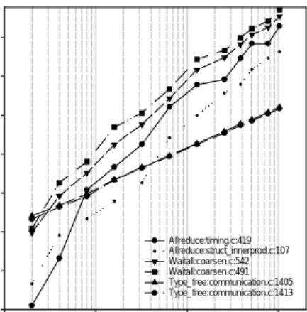
Allreduce:main.f:1025 immediately after the first one. Number of Tasks 1 10 100 1000 A g g regate T ime (m illis ecs ) 1e+0 1e+1 1e+2 1e+3 1e+4 1e+5 1e+6 1e+7 Allreduce:timing.c:419 Allreduce:struct_innerprod.c:107 Waitall:coarsen.c:542 Waitall:coarsen.c:491 Type_free:communication.c:1405 Type_free:communication.c:1413
Figure 13: Select call sites for SMG2000.
SMG2000 [2] is a parallel semicoarsening multigrid solver for the linear systems arising from finite difference, finite volume, or finite element discretizations of the diffusion equation,
f
u
u
D
∇
+
=
⋅
∇
(
)
σ
on logically rectangular grids. The code solves both 2D and 3D problems with discretization stencils of up to 9-point in 2D and up to 27-point in 3D. This code is a distributed memory application based on C and MPI. Note that the SMG2000 application includes the setup and solve of the linear system. In many applications, the setup can be performed once, and its cost amortized over many solves.SMG2000 scaling suffers from several collective operations. Four of the six operations are collectives with two Waitalls also having a strong positive correlation. Surprisingly, the SMG2000 rank correlation shows a large gap between positive and negative correlated operations. Six communication operations are strongly correlated to the number of tasks, where the lowest positive coefficient is 0.62. Figure 13 clarifies this difference. As before, these collective operations consume a very small portion of the communication time at 2 tasks and then they rise to the top positions at 1024 tasks. Once again, rank correlation has helped to identify the call sites that grow to consume more communication time as the number of tasks grow.
Number of Tasks 1 10 100 1000 A g gre g a te Time (m il lis ec s ) 1e-1 1e+0 1e+1 1e+2 1e+3 1e+4 1e+5 1e+6 1e+7 1e+8 Barrier:mpi_stuff.f:337 Bcast:mpi_stuff.f:248 Send:mpi_stuff.f:128 Recv:mpi_stuff.f:155 Comm_size:mpi_stuff.f:36
Figure 14: Select call sites for Sweep3D.
Sweep3D [12] is a solver for the 3-D, time-independent, particle transport equation on an orthogonal mesh. The solver computes along wavefronts in the mesh in eight diagonal directions through the cube. This code is built on FORTRAN and MPI.
Sweep3D scaling mirrors our earlier analysis where two collectives emerge to dominate practically all of the communication time. Unfortunately, Sweep3D wraps MPI communication routines in its own communication procedures, so all of the communication performance data is mapped into seven operations. Effectively, our data needs one more level of from the stack, so that it can discriminate among calls to these user-defined abstractions. We are currently implementing this feature.
4.4 Observations
The evaluation of our proposed technique for scalability analysis on nine applications produces several interesting observations. First, rank correlation of the number of tasks with the ratio of call site times to the overall communication time clearly identifies trends in the communication operations of the applications we evaluated. In our examples, this automated technique highlighted the communication operations whose aggregate time grows as the number of tasks increase.
Second, this type of correlation identifies call sites that simpler methods of analysis would not. Simply put, our analysis extracts trends from the data that could be easily overlooked by just looking at one experiment at a large task count. We can apply rank correlation to a large set of experiments and allow it to grade call sites based on all the evidence that it is presented.
Third, rank correlation is necessary in our example to remove outliers and to map the data into a normal distribution; however, the rank transformation discards some useful information including the magnitude of the variance. For instance, this conversion makes two sets of monotonically-increasing data samples exactly the same even though one set might change by a factor of 100 more than the other set. Still, the rank transformation eliminates more concerns than it introduces. It safely guarantees a normal distribution and it controls outliers.
Finally, it is important to note that both positive and negative correlation provides useful information. For instance, in the case of NAS FT, these correlations unmistakably separated the collective operations into two groups.
On reflection, our technique could benefit from several improvements as well. In particular, our analysis of Sweep3D was thwarted by the aliasing of performance data into the user-defined communication wrappers.
Our experiences also indicate that although this analysis uses only timing data, it can serve as a first-order approximation at scalability and other performance problems. With this information a user can easily interrogate the original data, or perform a trace of the offensive operations for more detailed performance data.
5 CONCLUSIONS
In this paper, we have proposed and evaluated a novel technique for identifying communication operations that scale poorly. Our technique uses non-parametric (or rank) correlation of the number of tasks to the ratio of the time for individual communication operations to the overall communication time. Our initial results with these applications on up to 1024 processors show that our correlation technique automatically and correctly identifies the poorly scaling operations in every case. We have also successfully
used this technique to analysis applications with 1536 processors on the ASCI White initial delivery system and with over two hundred individual MPI call sites. More importantly, our technique identifies performance problems in a way that a user can easily relate to the design of their application. Our experiments showed that our technique extracts trends from the performance data that are very important, but not obvious. Our experiments also show that similar communication operations do not scale similarly. Accordingly, we are also investigating automated techniques that robustly discover other performance phenomena, which include poor load-balancing and inadequate overlap of computation with communication.
ACKNOWLEDGEMENTS
This work was performed under the auspices of the U.S. Dept. of Energy by University of California LLNL under contract W-7405-Eng-48. LLNL Document Number UCRL-JC-142611.
REFERENCES
[1] D. Bailey, E. Barszcz et al., “The NAS Parallel Benchmarks (94),” NASA Ames Research Center, RNR Technical Report RNR-94-007, 1994.
[2] P.N. Brown, R.D. Falgout, and J.E. Jones, “Semicoarsening multigrid on distributed memory machines,” SIAM Journal on Scientific Computing, 21(5):1823-34, 2000.
[3] A.C. Calder, B.C. Curtis et al., “High-Performance Reactive Fluid Flow Simulations Using Adaptive Mesh Refinement on Thousands of Processors,” Proc. SC2000: High Performance Networking and Computing Conf. (electronic publication), 2000.
[4] M. Calzarossa, L. Massari et al., “Parallel performance evaluation: the Medea tool,” Proc. High-Performance Computing and Networking (HPCN Europe 1996), 1996, pp. 522-9.
[5] S.K. Card, B. Shneiderman, and J.D. Mackinlay, Readings in information visualization: using vision to think. San Francisco, CA: Morgan Kaufmann Publishers, 1999. [6] D.E. Culler, J.P. Singh, and A. Gupta, Parallel computer
architecture: a hardware software approach. San Francisco: Morgan Kaufmann Publishers, 1999.
[7] I. Foster, Designing and building parallel programs: concepts and tools for parallel software engineering. Reading, MA: Addison-Wesley, 1995.
[8] G.A. Geist, M.T. Heath et al., “A Users' Guide to PICL - A Portable Instrumented Communication Library,” Oak Ridge National Laboratory, P.O.Box 2009, Bldg. 9207-A, Oak Ridge, TN 37831-8083 1991.
[9] W. Gropp, E. Lusk, and A. Skjellum, Using MPI: portable parallel programming with the message-passing interface, 2nd ed. Cambridge, MA: MIT Press, 1999.
[10] M.T. Heath, A.D. Malony, and D.T. Rover, “Parallel performance visualization: from practice to theory,” IEEE Parallel & Distributed Technology: Systems & Applications, 3(4):44-60, 1995.
[11] R.A. Johnson and D.W. Wichern, Applied Multivariate Statistical Analysis, 4 ed. Englewood Cliffs, New Jersey, USA: Prentice-Hall, 1998.
[12] K.R. Koch, R.S. Baker, and R.E. Alcouffe, “Solution of the First-Order Form of the 3-D Discrete Ordinates Equation on a Massively Parallel Processor,” Trans. Amer. Nuc. Soc., 65(198), 1992.
[13] V. Kumar, A. Grama et al., Introduction to parallel computing: design and analysis of algorithms. Redwood City, Calif.: Benjamin/Cummings Pub. Co., 1994.
[14] V. Kumar and A. Gupta, “Analyzing Scalability of Parallel Algorithms and Architectures,” Journal of Parallel and Distributed Computing, 22(3):379-91, 1994.
[15] A.A. Mirin, R.H. Cohen et al., “Very High Resolution Simulation of Compressible Turbulence on the IBM-SP System,” Proc. SC99: High Performance Networking and Computing Conf. (electronic publication), 1999.
[16] W.H. Press, S.A. Teukolsky et al., Numerical recipes in C: the art of scientific computing, 2nd , rev. ed. Cambridge Cambridgeshire; New York: Cambridge University Press, 1997.
[17] D.A. Reed, R.A. Aydt et al., “An Overview of the Pablo Performance Analysis Environment,” Department of Computer Science, University of Illinois, 1304 West Springfield Avenue, Urbana, IL 61801 1992.
[18] D.A. Reed, O.Y. Nickolayev, and P.C. Roth, “Real-Time Statistical Clustering and for Event Trace Reduction,” J. Supercomputing Applications and High-Performance Computing, 11(2):144-59, 1997.
[19] S. Shende, A.D. Malony et al., “Portable profiling and tracing for parallel, scientific applications using C++,” Proc. SIGMETRICS Symp. Parallel and Distributed Tools (SPDT), 1998, pp. 134-45.
[20] M. Snir, S. Otto et al., Eds., MPI--the complete reference, 2nd ed. Cambridge, MA: MIT Press, 1998.
[21] J. Stasko, J. Domingue et al., Eds., Software Visualization: Programming as a Multimedia Experience,. Cambridge, MA: MIT Press, 1998.
[22] J.S. Vetter, “Performance Analysis of Distributed Applications using Automatic Classification of Communication Inefficiencies,” Proc. ACM Int'l Conf. Supercomputing (ICS), 2000, pp. 245 - 54.
[23] J.S. Vetter and D. Reed, “Managing Performance Analysis with Dynamic Statistical Projection Pursuit,” Proc. SC99: High Performance Networking and Computing Conf. (electronic publication), 1999.
[24] F. Wong, R. Martin et al., “Architectural Requirements and Scalability of the NAS Parallel Benchmarks,” Proc. SC99: High Performance Networking and Computing Conf. (electronic publication), 1999.