Procedia Computer Science 17 ( 2013 ) 514 – 522
1877-0509 © 2013 The Authors. Published by Elsevier B.V.
Selection and peer-review under responsibility of the organizers of the 2013 International Conference on Information Technology and Quantitative Management
doi: 10.1016/j.procs.2013.05.066
Information Technology and Quantitative Management , ITQM 2013
Exploring determinants of inflation in China based on
L
1
-
-twin
support vector regression
Ya-Fen Ye
a, Hui Cao
b,∗, Lan Bai
c, Zhen Wang
c, Yuan-Hai Shao
aaZhijiang College, Zhejiang University of Technology, Hangzhou, 310024, P.R.China bCollege of Sciece,Zhejiang University of Technology, Hangzhou, 310023, P.R.China
cCollege of Mathematics, Jilin University, Changchun, 130012, P.R.China
© 2013 The Authors. Published by Elsevier B.V.
Selection and peer-review under responsibility of the organizers of the 2013 International Conference on Information Technology and Quantitative Management
Abstract
As a novel feature selection approach, L1-norm-twin support vector regression(L1-- TSVR )is proposed in this paper to
investigate determinants of cost-push inflation in China. Compared withL2-ε-TSVR , ourL1-- TSVR not only can fit function
well, but also can do feature ranking. The computational results of inflation forecasts demonstrate that our L1-- TSVR
derives much smaller root mean squared error (RMSE) than the forecasts generated from ordinary least square (OLS) model. Furthermore, the feature selection results indicate that the most significant explanatory factor for the inflation in China is the housing sales price index. Therefore, the housing market do have an important impact on the inflation in China.
Keywords: support vector machines,L1-ε-TSVR, cost-push factors, Chinese inflation
1. Introduction
Inflation has played a prominent role in financial economics for a long time. The literatures by identify-ing important determinants of inflation in China has been growidentify-ing rapidly in recent years[1–3]. However, these econometric models rely on some strong assumptions and ignore some real economic information. While sup-port vector regression (SVR) algorithm, being computationally powerful tools, can overcome this shortcoming. SVR is based on statistical learning theory and has been successfully applied in many important fields including economics, engineering and bioinformatics, etc [4, 5].
There has been some extensive models of SVR such as least square support vector regression (LS-SVR) [6],
twin support vector regression (TSVR)[7],ε- twin support vector regression (ε-TSVR) [8] and so on. Different
from SVR,ε-TSVR determines a pair ofε-insensitive proximal functions by solving two related SVM-type
prob-lems, each of which is smaller than that in a classical SVR. In fact,ε-TSVR inspire by the twin support vector
machines [9–14]. Thus,ε-TSVR has more powerful study ability and faster speed than SVR. Althoughε-TSVR
achieves good performance, it is less robust because the square of theL2norm distance of the residuals is sensitive
to the large errors [15–17]. This fact motivates us to formulateε-TSVR as two linear programming problems
∗Corresponding author. Tel.:+086-0571-87313643; fax:+086-0571-87313643 URL:[email protected](Hui Cao)
Open access under CC BY-NC-ND license.
by using theL1 norm distance, called L1-norm- twin support vector regression (L1--TSVR). The use of
L1-norm distance in the-TSVR as opposed to the square of theL2-norm leads to the robustness, which makes the
L1--TSVR own the better generalization ability.
In this paper, in order to verify the effective of theL1--TSVR, we adoptL1-- TSVR to explore the important
determinants of the inflation in China. We use consumer price index (CPI) as the dependent variable, and test 5 cost-push factors including the housing sales price index, the producer price index (PPI), the international crude oil price, the agriculture and sideline products purchasing price index, and the ferrous metals price index. Specif-ically,the operation is divided into two parts. Firstly, the computational results of inflation forecasts demonstrate
that our L1-- TSVR derives much smaller root mean squared error (RMSE) than the forecasts generated from
ordinary least square (OLS) model, which indicates that ourL1-- TSVR is an efficient algorithm for the inflation
forecasts. Then, we focus on these 5 cost-push factors to determine the important determinant of Chinese
infla-tion. The experimental result of our linearL1--TSVR indicates that the most significant explanatory factor for
the inflation in China is the housing sales price index.
The remainder of this paper is structured as follows: the following section introducesε-TSVR. In section 3
we discuss our L1--TSVR . The artificial datasets experiments are described in section 4. Section 5 contains
the inflation forecasts of our L1-- TSVR and the ordinary least square (OLS) model, and discuss important
determinants of inflation in China. Section 6 concludes this paper.
2. ε-twin support vector regression
In this section, we introduceε-twin support vector regression (ε-TSVR). Consider the following regression
problem in then-dimensional real spaceRn, suppose that the training set is denoted by (A,Y), whereAis al×n
matrix and the i-th rowAi ∈ Rn represents thei-th training sample Y = (y1;y2;· · ·;yl) ∈ Rn ×1 denotes the
response vector of training sample,i=1,2,· · ·,l. 2.1. Linearε-TSVR
Following the literature of [8],ε-TSVR finds the following twoε-insensitive proximal functions
f1(x)=w1x+b1 and f2(x)=w2x+b2. (1)
By introducing the regularization terms 1
2(w1w1+b21) and 12(w2w2+b21), the slack variablesξ,ξ∗,ηandη∗, the primal problems can be expressed as
min w1,b1,ξ,ξ∗ 1 2c3(w1w1+b 2 1)+ 1 2ξ∗ξ∗+c1eξ, s.t. Y−(Aw1+eb1)=ξ∗,Y−(Aw1+eb1)≥ −ε1e−ξ, ξ≥0, (2) and min w2,b2,η,η∗ 1 2c4(w2w2+b22)+ 1 2η∗η∗+c2eη,
s.t. (Aw2+eb2)−Y =η∗,(Aw2+eb2)−Y≥ −ε2e−η, η≥0, (3)
wherec1,c2,c3,c4,ε1andε2are positive parameters. Then, the dual problems of the problem (2) and (3) are as
follows max α − 1 2αG(GG+c3I)− 1Gα+YG(GG+c 3I)−1Gα−(eε1+Y)α s.t. 0≤α≤c1e, (4) max γ − 1 2γG(GG+c4I)−1Gγ−YG(GG+c4I)−1Gγ+(Y−eε2)γ s.t. 0≤γ≤c2e, (5)
whereαandγare the Lagrange multipliers,G=[A e]. The augmented vectorv1=[w1 b1],andv2 =[w2 b2]
are given by
Once the solutions (w1,b1) and (w2,b2) of the problems (2) and (3) are obtained from the solutions of (4)
and (5), the two proximal functions f1(x) and f2(x) are obtained. Then the estimated regressor is constructed as
follows f(x)= 1 2(f1(x)+f2(x))= 1 2(w1+w2) x+1 2(b1+b2). (7) 2.2. Kernelε-TSVR
In order to extend the above (4) and (5) to nonlinear regressors, consider the following two ε-insensitive
proximal functions
f1(x)=K(x,A)u1+b1,f2(x)=K(x,A)u2+b2, (8)
whereKis a kernel.
By introducing the slack variablesξ,ξ∗,ηandη∗, the primal problems can be expressed as
min u1,b1,ξ 1 2c3(u1u1+b21)+ 1 2ξξ∗+c1eξ, s.t. Y−(K(A,A)u1+eb1)≥ −ε1e−ξ, ξ≥0,Y−(K(A,A)u1+eb1)=ξ∗, (9) and min u2,b2,η 1 2c4(u2u2+b22)+ 1 2ηη∗+c2eη,
s.t. (K(A,A)u1+eb1)−Y≥ −ε2e−η, η≥0,(K(A,A)u2+eb2)−Y =η∗, (10)
wherec1,c2,c3andc4are positive parameters.
Then, the dual problem of (9) is obtained as follows max α − 1 2αH(HH+c3I)− 1Hα−(eε 1+Y)α+YH(HH+c3I)−1Hα s.t. 0≤α≤c1e, (11) and max γ − 1 2γH(HH+c4I)− 1Hγ+(Y−eε 2)γ−YH(HH+c4I)−1Hγ s.t. 0≤γ≤c2e, (12)
whereαandγare the Lagrange multipliers. The augmented vectorv1=[u1 b1]andv2=[u2 b2]are given by
v1=(HH+c3I)−1H(Y−α) andv2=(HH+c4I)−1H(Y+γ). (13)
Once the solutions (u1,b1) and (u2,b2) of the problems (9) and (10) are obtained from the solutions of (11)
and (12), the two functions f1(x) and f2(x) are obtained. Then the estimated regressor is constructed as follows
f(x)= 1 2(f1(x)+f2(x))= 1 2(u 1 +u2)K(A,x)+ 1 2(b1+b2). (14)
3. L1-norm-twin support vector regression 3.1. Linear L1-norm-twin support vector regression
By replacing the square of theL2-norm in the quadratic program (4) or (5) with theL1-norm, we obtain the
linearL1--twin support vector regression(L1--TSVR) as follows
min w1,b1,ξ1 ||w1||1+|b1|+c11||Aw1+b1e−Y||1+c12eξ1, s.t. Aw1+b1e−Y≤ε1e+ξ1, ξ1≥0, (15) and min w2,b2,ξ2
||w2||1+|b2|+c21||Aw2+b2e−Y||1+c22eξ2, s.t. Aw2+b2e−Y≥ −ε2e−ξ2, ξ2≥0,
wherec11,c12,c21,c22are positive parameters, andξ1andξ2are the slack vectors. In order to solve (15), we firstly introduce the following definitions as
u1=[w1;b1]=p1−q1,B1=[A,e],Aw1+b1e−Y =B1u1−Y =s1−t1, (17)
wherer1,s1,p1,q1are all nonnegative auxiliary vectors. Then, we can re-express the minimization problem (15)
as follows min p1,q1,s1,t1,ξ1 e(p1+q1)+c11e(s1+t1)+c12eξ1, s.t. s1−t1≤ε1e+ξ1,B1(p1−q1)−Y =s1−t1,p1,q1,s1,t1, ξ1≥0. (18) In the same way, the minimization problem (16) can re-express as follows
min p2,q2,s2,t2,ξ2 e(p2+q2)+c21e(s2+t2)+c22eξ2, s.t. s2−t2≥ −ε2e−ξ2,B1(p2−q2)−Y =s2−t2,p2,q2,s2,t2, ξ2≥0, (19) whereu2=[w2;b2]=p2−q2andB1u2−Y=s2−t2.
The (18) and (19) are standard linear program and can be solved by many LP solvers.Once the problems in
(15) and (16) are solved, the two function f1(x) andf2(x) are obtained. Then the estimated regressor is constructed
as follows f(x)= 1 2(f1(x)+f2(x))= 1 2(w1+w2) x+1 2(b1+b2). (20)
3.2. Nonlinear L1-norm-twin support vector regression
In order to extend our results to nonlinear regression, we first express the proximal functions in kernel space as follows
f1(x)=K(x,A)w1+b1,f2(x)=K(x,A)w2+b2. (21)
Then, following the same idea of linear L1--TSVR, we give the model for nonlinear L1--TSVR as the
following two optimization problems min w1,b1,ξ1 ||w1||1+|b1|+c11||K(A,AT)w 1+b1e−Y||1+c12eξ1, s.t. K(A,AT)w1+b1e−Y ≤ε1e+ξ1, ξ1≥0, (22) and min w2,b2,ξ2 ||w2||1+|b2|+c21||K(A,AT)w 2+b2e−Y||1+c22eξ2, s.t. K(A,AT)w2+b2e−Y ≥ −ε2e−ξ2, ξ2≥0. (23)
The optimal solution [w1;b1] and [w2;b2] for (22) and (23) following similar procedure in linearL1--TSVR
are as follows min p1,q1,s1,t1,ξ1 e(p1+q1)+c11e(s1+t1)+c12eξ1, s.t. s1−t1≤ε1e+ξ1,B2(p1−q1)−Y =s1−t1, p1,q1,s1,t1, ξ1≥0, (24) min p2,q2,s2,t2,ξ2 e(p2+q2)+c21e(s2+t2)+c22eξ2, s.t. s2−t2≥ −ε2e−ξ2,B2(p2−q2)−Y=s2−t2, , p2,q2,s2,t2, ξ2≥0, (25) whereB2=[K(A,AT),e] ,B2u1−Y =s1−t1,B2u2−Y=s2−t2. The resulting regression function can be express by
f(x)=1 2(f1(x)+f2(x))= 1 2(w T 1 +wT2)K(A,x)+ 1 2(b1+b2). (26)
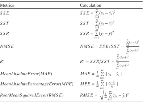
Table 1. Performance metrics and their calculations. Metrics Calculation S S E S S E=m i=1 (yi−yˆi)2 S S T S S T =m i=1 (yi−y)¯2 S S R S S R=m i=1 (ˆyi−y)¯2 N MS E N MS E=S S E/S S T = m i=1( yi−yˆi)2 m i=1 (yi−y¯)2 R2 R2=S S R/S S T = m i=1(ˆ yi−¯y)2 m i=1 (yi−¯y)2 MeanAbsoluteError(MAE) MAE= 1 m m i=1| yi−yˆi| MeanAbsolutePercentageError(MPE) MPE= 1 m m i=1| yi−yˆi yi | RootMeanS quaredError(RMS E) RMS E= 1 m m i=1 (yi−yˆi)2 4. Numerical test
In this section, we use the artificial datasets to test the performance of ourL1--TSVR. The values of the
pa-rameters in our method are obtained through searching in the range 2−8to 28by tuning a set comprising of random
10% of the dataset. In our experiments, we setc11 = c21,c12 = c22 andε1 = ε2 to degrade the computational
complexity of parameter selection. Some evaluation criteria are introduced in Table 1. Without loss of generality,
letlbe the number of training samples, and denotemas the number of testing samples, ˆyias the prediction value
ofyi, and ¯y=m1iyias the average value ofy1,· · ·,ym.
We use the sinc function to test the performance of our L1--TSVR, which is defined as: y = sin(xx), x ∼
U[−4π,4π].To effectively reflect the performance of our method, training data samples are polluted by some
different kinds of noises, including the Gaussian noises with zero means and the uniformly distributed noises.
Specially, we have the following training samples (xi,yi): yi= sin(xi) xi +ξi, xi∼U[−4π,4π], ξi∼N(0,0.12), (27) yi= sin(xi) xi +ξ i, xi∼U[−4π,4π], ξi∼N(0,0.22), (28) yi= sin(xi) xi +ξi, xi∼U[−4π,4π], ξi∼U[0,0.1], (29) yi= sin(xi) xi +ξi, xi∼U[−4π,4π], ξi∼U[0,0.2], (30)
whereU[a,b] andN(c,d2) represent the uniformly random variable in [a,b] and the Gaussian random variable
with meanscand varianced2, respectively. Our datasets consist of 252 training samples and 503 test samples.
Now, we show some comparisons of ourL1--TSVR withε-TSVR. Fig. 1(a-d) illustrate the one-run
simu-lation results for these four different types of noises. Obviously, ourL1--TSVR derives better approximations
compared withε-TSVR in these four cases. The results of the performance criteria are listed in Table 2. It has been
seen that ourL1--TSVR derives the smaller SSE, which indicates that the statistical information in the training
−15 −10 −5 0 5 10 15 −0.4 −0.2 0 0.2 0.4 0.6 0.8 1 1.2 1.4 Sinc(x) Samples 1 norm ETSVR 2 norm ETSVR Down−1 norm ETSVR Up−1 norm ETSVR
(a) −15 −10 −5 0 5 10 15 −0.5 0 0.5 1 1.5 Sinc(x) Samples 1 norm ETSVR 2 norm ETSVR Down−1 norm ETSVR Up−1 norm ETSVR
(b) −15 −10 −5 0 5 10 15 −0.4 −0.2 0 0.2 0.4 0.6 0.8 1 1.2 1.4 Sinc(x) Samples 1 norm ETSVR 2 norm ETSVR Down− 1 norm ETSVR Up−1 norm ETSVR
(c) −15 −10 −5 0 5 10 15 −0.4 −0.2 0 0.2 0.4 0.6 0.8 1 1.2 1.4 Sinc(x) Samples 1 norm ETSVR 2 norm ETSVR Down−1 norm ETSVR Up−1 norm ETSVR
(d)
Table 2. Result comparisons of ourL1--TSVR andε-TSVR on artificial datasets with the RBF kernel.
Dataset Regressor SSE NMSE R2 CPU .
(27) L1--TSVR 3.149 0.055 0.877 2.201 (27) ε-TSVR 2.037 0.036 0.932 2.111 (28) L1--TSVR 22.784 0.315 0.680 1.860 (28) ε-TSVR 22.692 0.314 0.721 0.007 (29) L1--TSVR 0.444 0.008 0.991 1.556 (29) ε-TSVR 0.669 0.012 0.935 0.114 (30) L1--TSVR 1.905 0.033 0.971 1.779 (30) ε-TSVR 1.800 0.032 0.966 0.007
Table 3. Results of ourL1--TSVR and the OLS model .
Regressor MAE MPE RMSE
L1--TSVR 0.916 0.008 1.123
OLS 1.293 0.0125 1.503
5. Determinants of Chinese inflation
5.1. Data
The aim of this part is to explore important determinants of inflation in China. We use national-level monthly time series from July 2005 to October 2012, with 88 observations for each variable. For the dependent variable, we use the consumer price index (CPI) movement as the measure of the inflation. The cost factors of inflation are the housing sales price index, the producer price index (PPI), the international crude oil price, the agriculture and sideline products purchasing price index, the ferrous metals price index. International crude oil price is taken
from U.S. Energy Information Administration (EIA)(http://www.eia.gov/), and the other indexes are obtained
from national statistic bureau of China (http://www.stats.gov.cn/). All these indicators are listed in Table 3.
0 2011m6 2011m8 2011m10 2011m12 2012m2 2012m4 2012m6 2012m8 2012m10 101 102 103 104 105 106 107 108 Actual data OLS L 1−ε−TSVR
Fig. 2. The actual and forecasting inflation series.
Firstly, we test the forecasting performance of ourL1--TSVR, which is compared with the ordinary least
square (OLS) model. The evaluation criterions and their definitions are specified in Table 1. The dataset is divided into two parts: the training samples and the test samples. Specially, the last 18 monthly data of the inflation data is used to compute forecast error and test statistics.
The forecasting performance of ourL1--TSVR and the OLS model are listed in Table 3. From the Table 3
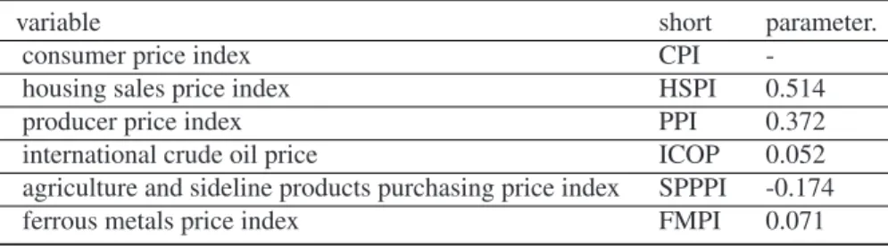
Table 4. Variables list.
variable short parameter.
consumer price index CPI
-housing sales price index HSPI 0.514
producer price index PPI 0.372
international crude oil price ICOP 0.052
agriculture and sideline products purchasing price index SPPPI -0.174
ferrous metals price index FMPI 0.071
L1--TSVR delivers much lower MAE, MPE and RMSE than the OLS model. Thus, the traditional OLS model
does not perform well in inflation forecasts for China. OurL1--TSVR inflation forecasts can outperform the OLS
forecasts derived in this paper. The actual and forecasting inflation series over the predicting period are shown
in Fig. 2. Obviously, compared to the OLS model, ourL1--TSVR delivers relatively more accurate forecasts of
inflation for China, which indicate that ourL1-ε-TSVR is an efficient method for the inflation forecasting.
Then, we adopt ourL1--TSVR with linear terms to test the impact of major cost factors on the inflation
in China. Shown by the estimated parameter value as listed in Table 4, the most significant explanatory factor for Chinese inflation is the housing sales price index. This result indicates that the developments in the Chinese housing market do have an important impact on inflation. PPI also is a significant explanatory factor for Chinese inflation. The agriculture and sideline products purchasing price enters the model with a negative parameter,
which indicates that it has negative effects on the Chinese inflation. The international crude oil price and the
ferrous metals price have rather weak explanatory power on the inflation.
6. Conclusion
A new version ofL1--TSVR is proposed in this paper to explore the important determinants of inflation in
China. Specifically, the operation is divided into two parts. Firstly, the computational results of inflation
fore-casts demonstrate that ourL1-- TSVR derives much smaller root mean squared error (RMSE) than the forecasts
generated from ordinary least square (OLS) model, which indicates that ourL1-- TSVR is an efficient algorithm
for the inflation forecasts. Then, we focus on these 5 cost-push factors to determine the important determinant of
Chinese inflation. The feature selection results of our linearL1--TSVR show that the most significant explanatory
factor for the inflation in China is the housing sales price index, which indicates the housing market do have an important impact on the inflation in China. It should be pointed out that this paper only focuses on the cost-push factors on Chinese inflation, while other important factors such as the demand-pull factors and the money factors are ignored. Such consideration will be our continue research points.
Acknowledgments
This work is supported by the National Natural Science Foundation of China (No.11201426, No. 10971223 and No. 11071252), the Zhejiang Provincial Natural Science Foundation of China (No.LQ12A01020), the Sci-ence and Technology Foundation of Department of Education of Zhejiang Province (No. Y201225256 and No.Y201225179), and the Graduate Innovation Fund of Jilin University (No.20121053).
References References
[1] W.Q. Tang, L.B. Wu, Z.X. Zhang, Oil price shocks ans their shot-and long-term effects on the Chinese economy. Energy Economics, 2010, 32:s3-s14
[3] Z.H. Ding, M.H. Zhou, B. Ning, Research on the inflencing effect of coal price fluctuation on CPI of China. Energy Procedia, 2011, 5:1508-1513.
[4] N. Y. Deng, Y. J. Tian, C. H. Zhang, Support Vector Machines: Optimization Based Theory, Algorithms, and Extensions, CRC Press, 2012.
[5] Y. Tian, Y. Shi, X. Liu, Recent advances on support vector machines research. Technological and Economic Development of Economy, 2012, 18(1):5-33.
[6] JAK Suykens, J Vandewalle, Least squares support vector machine classifiers. Neural Process Letter, 1999, 9:293-300. [7] X.J. Peng, TSVR: An efficient Twin Support Vector Machine for regression. Neural Networks, 2010 23:365-372.
[8] Y.H. Shao, C.H. Zhang, Z.M. Yang, L. Jing, N.Y. Deng, Anε-twin support vector machine for regression. Neural Comput Applic, 2012, doi 10.1007/s00521-012-0924-3
[9] Z.Q. Qi, Y.J. Tian, Y. Shi, Twin support vector machine with Universum data. Neural Networks, 2012, 36C:112-119.
[10] Z. Qi, Y. Tian, and Y. Shi, Laplacian Twin Support Vector Machine for Semi-supervised Classification, Neural Networks, vol. 35, pp. 46-53, 2012
[11] Z. Qi, Y. Tian, and Y. Shi, Structural Twin Support Vector Machine for Classification, Knowledge-Based Systems, 2013, DOI: 10.1016/j.knosys.2013.01.008
[12] Y.H. Shao, C.H. Zhang, X.B. Wang, N.Y. Deng, Improvements on twin support vector machines. IEEE transactions on neural networks, 2011, 22:962-968.
[13] Y.H. Shao, N.Y. Deng, Z.M. Yang, Least squares recursive projection twin support vector machine for classification. Pattern Recognition, 2012, 45:2299-2307.
[14] Y.H. Shao, N.Y. Deng, Z.M. Yang, W.J. Chen, Z. Wang, Probabilistic outputs for twin support vector machines. Knowledge Based Systems, 2012, 33:145-151.
[15] Y.H. Shao, Z. Wang, W.J. Chen, N.Y. Deng, A regularization for the projection twin support vector machine. Knowledge-Based Systems, 2013, 37:203-210.
[16] Z.Q. Qi, Y.J. Tian, Y. Shi, Robust twin support vector machine for pattern classification. Pattern Recognition, 2013, 46(1):305-316. [17] Y.H. Shao, N.Y. Deng, W.J. Chen, Z. Wang, Improved generalized eigenvalue proximal support vector machine. IEEE Signal Processing