HAL Id: hal-02385387
https://hal.archives-ouvertes.fr/hal-02385387
Submitted on 28 Nov 2019
HAL
is a multi-disciplinary open access
archive for the deposit and dissemination of
sci-entific research documents, whether they are
pub-lished or not. The documents may come from
teaching and research institutions in France or
abroad, or from public or private research centers.
L’archive ouverte pluridisciplinaire
HAL, est
destinée au dépôt et à la diffusion de documents
scientifiques de niveau recherche, publiés ou non,
émanant des établissements d’enseignement et de
recherche français ou étrangers, des laboratoires
publics ou privés.
Convergence of the two-dimensional random walk
loop-soup clusters to CLE
Titus Lupu
To cite this version:
Titus Lupu. Convergence of the two-dimensional random walk loop-soup clusters to CLE.
Jour-nal of the European Mathematical Society, European Mathematical Society, 2019, 21, pp.1201-1227.
�10.4171/JEMS/859�. �hal-02385387�
CONVERGENCE OF THE TWO-DIMENSIONAL RANDOM WALK LOOP-SOUP CLUSTERS TO CLE
TITUS LUPU
CNRS and LPSM, UMR 8001, Sorbonne Universit´e, 4 place Jussieu, 75252 Paris cedex 05, France
Abstract. We consider the random walk loop-soup of sub-critical intensity parameter on the discrete half-planeH:=Z×N. We look at the clusters of discrete loops and show that the scaling limit of the outer boundaries of outermost clusters is a CLEκConformal loop ensemble.
1. Introduction
One can naturally associate to a wide class of Markov processes an infinite measure on time-parametrised loops. Roughly speaking, given a locally compact second-countable spaceS, a Markov process (Xt)0≤t<ζ
onS, defined up to a killing timeζ∈(0,+∞], with transition densitiespt(x, y) with respect someσ-finite
measure m(dy), incorporating the killing if there is one, and with bridge probability measuresPt x,y(·),
where the bridges are conditioned onζ > t, the loop measure associated toX is
(1.1) µ(·) = Z x∈S Z t>0 Ptx,x(·)pt(x, x) dt t m(dx).
See [8] for the precise setting and definition. APoisson ensemble of Markov loopsorloop-soupof intensity parameterα >0 is a Poisson point process of loops of intensityαµ. It is a random countable collection of loops. These loop-soups satisfy some universal properties, one of which is the relation to the Gaussian free field at intensity parameterα = 1/2 [3, 9]. We will deal with the clusters of loops. Two loops γ andγ0 in a loop-soup belong to the same cluster if there is a chain of loopsγ0, . . . , γj such thatγ0=γ,
γj=γ0 andγi and γi−1 visit a common point inS.
We will consider loop-soups in three different settings. In the first one, on the continuum half-plane
H={=(z)>0} ⊂C, we will consider the loop-soups associated to the Brownian motion onHkilled at
the first hitting time of the boundary Rand denote them LH
α. These two-dimensional Brownian
loop-soups were introduced by Lawler and Werner in [5] and used by Sheffield and Werner in [14] to give a construction of Conformal loop ensembles (CLE). In (1.1) we use the same normalisation of the loop measure as in [5], [14], [3] or [4]. However, contrary to what is claimed in [14], the intensity parameter αis not equal to thecentral charge c. The central charge is a notion that comes from Conformal Field Theory and representations of Virasoro algebra. Actually,
α= c 2.
The 1/2 factor was pointed out by Werner in a private communication. It also appears in Lawler’s work [6]. The confusion originates from the article [5]. There the authors consider a Brownian loop soup in the half-plane and a continuous path cutting the half-plane, parametrised by the half-plane capacity. For such a path the half-plane capacity at time tequals 2t . It discovers progressively new Brownian loops and the authors map these loops conformally to the origin. In Theorem 1 they identify the processes of these conformally mapped Brownian loops to be a Poisson point process with intensity proportional to the Brownian bubble measure. In the identification of the intensity there is a factor 2 missing. Actually, in the article [5], Theorem 1 is inconsistent with Proposition 11.
In the second setting, on the discrete rescaled half-plane
Hn:= 1 nZ × 1 nN ,
E-mail address:[email protected].
2010Mathematics Subject Classification. Primary 60G15; 60J67; 60K35; 82B20; Secondary 82B27.
Key words and phrases. Conformal loop ensemble; Gaussian free field; loop-soup; metric graph; Poisson ensemble of Markov loops.
we will consider the loop-soups associated to the nearest neighbours Markov jump process with uniform transition rates and killed at the first hitting time of the boundary 1nZ× {0}. We will denote these
loop-soupsLHn
α . The loop-soups associated to Markov jump processes on more general electrical networks were
studied by Le Jan in [3]. If one forgets the parametrisation by continuous time and the ”loops” that visit only one vertex, these are exactly the random walk loop-soups studied by Lawler and Trujillo-Ferreras in [4]. See also [7], Section 9.
In the third setting, we will use the metric (or cable) graphseHn associated toHn: each ”discrete” edge
{(ni,nj),(i+1n ,jn)}or{(ni,nj),(ni,j+1n )}is replaced by a continuous line of length n1. Let (BeHn
t )0≤t<ζn be
the Brownian motion on eHn (cable process) killed at reaching the boundary, that is to say the vertices
1
nZ× {0}and all the lines joining ( i
n,0) to ( i+1
n ,0). One can find a construction of (B
eHn
t )0≤t<ζn in [9].
Inside each line segment,BeHn
t evolves like a one-dimensional Brownian motion. After reaching a vertex,
the process makes Brownian excursions in each of the four possible directions before hitting the next vertex. Each direction has an equal rate. (BeHn
2t)0≤t<ζn/2converges in law to the Brownian motion on the
half-planeHkilled at reachingR. We will denote byLeHn
α the loop-soups associated to (BeHtn)0≤t<ζn. The
loop-soups on metric graphs were first considered in [9]. We will use metric graphs because at intensity parameterα= 1/2 the probability that two points belong to the same cluster of loops can be explicitly expressed using a metric graph Gaussian free field. Indeed, the clusters of loops are then exactly the sign clusters of the Gaussian free field [9].
The discrete loopsLHn
α can be deterministically recovered from the metric graph loopsLeHαn. The first
are the trace on the vertices of the latter. In particular each cluster ofLHn
α is contained in a cluster of
LeHn
α , but the clusters ofLeHαn may be strictly larger [9].
c = 1 is the critical central charge for the Brownian loop percolation on H (or any other simply
connected proper subset of C). This means that the critical intensity parameter is α = 1/2. For
α > 1/2, LH
α has only one cluster everywhere dense in H. If α ∈ (0,1/2], there are infinitely many
clusters and each is bounded [14]. α= 1/2 is also the critical intensity parameter for the existence of an unbounded cluster of loops on discrete or metric graph half-planeHn respectivelyeHn [10, 9]. In all
three settings, forα∈(0,1/2], we will consider the collection of outer boundaries of outermost clusters (not surrounded by any other cluster) and denote it Fext(LSα), where S is H, Hn or eHn. Next we give
the formal definition of Fext(LSα). We consider the set of all points in Hvisited by a loop in LSα and
take its complement in H. This complement has only one unbounded connected component. We take the boundary inHof this connected component (by definition it does not intersectR). The elements of
Fext(LS
α) are the connected components of this boundary. We will call the elements ofFext(LSα)contours.
The contours are pairwise disjoint and non nested. See Figure 1 for a representation ofFext(LeHn α ).
The contours in Fext(LH
α), α ∈ (0,1/2], are non self-intersecting loops, and are equal in law to a
Conformal loop ensemble CLEκ,κ∈(8/3,4] [14]. The relation betweenαandκis given by
(1.2) 2α=c=(3κ−8)(6−κ) 2κ .
We will denote byκ(α) the value ofκcorresponding to a particular intensity parameterα. We will show that both Fext(LHαn) and Fext(LeHαn) converge in law to Fext(LHα)
(d)
= CLEκ(α) for α ∈ (0,1/2]. Observe thatκ(1/2) = 4 and Fext(LeH1n/2) and CLE4are both related to the Gaussian free field.
Fext(LeH1n/2) is the collection of outer boundaries of outermost sign clusters of a GFF on the metric graph e
Hn [9] and the CLE4 loops are in some sense zero level lines of the continuum GFF on H with zero
boundary conditions onR[11, 15, 1, 12, 13].
Next we define the notion of convergence we will use. dH will be Hausdorff distance on the compact
subsets ofH. We introduce the distanced∗H between finite collections of compact subsets ofH:
d∗H(K,K0) =
+∞ if|K| 6=|K0|, minσ∈Bij(K,K0)maxK∈KdH(K, σ(K)) otherwise,
where Kand K0 are finite collections of compact subsets and Bij(K,K0) is the set of all bijections from
K toK0. Givenz∈
H, we will denote by
Fext(LSα)(z)
Figure 1. Illustration of three clusters (thin full lines) of LeHn
α , two of them being
external and one being surrounded. The thick lines represent the elements ofFext(LeHn α).
the contour ofFext(LS
α) that contains or surroundsz, whenever it exists. It exists a.s. in the caseS=H.
Givenz1, . . . , zj ∈H, we will denote
Fext(LS
α)[z1, . . . , zj] :={Fext(LSα)(zi)|1≤i≤j}.
By the convergence in law ofFext(LHn
α ) andFext(LeHαn) toFext(LHα) we mean that for anyz1, . . . , zj∈H,
Fext(LHn
α )[z1, . . . , zj] andFext(LeHαn)[z1, . . . , zj] converge in law toFext(LHα)[z1, . . . , zj] for the distanced∗H.
So, the main result in this article is the following.
Theorem 1.1. Let α∈(0,1/2]. Fext(LαHn)and Fext(LeHαn) converge in law (in the above defined sense)
asn→+∞toFext(LHα), that is to say to a CLEκ(α) onH.
In the article [2] Van de Brug, Camia and Lis consider clusters of rescaled two-dimensional random walk loops that are not too small. Given T > 0 let LHn,T
α be the subset of LHαn consisting of random
walk loops that do at least T jumps. In [2] it is almost shown that forθ ∈(16/9,2) and α∈(0,1/2],
Fext(LHn,nθ
α ) converges in law to a CLEκ(α) process in the sense described previously. The result uses the approximation of ”not too small” Brownian loops by ”not too small” random walk loops obtained by Lawler and Trujillo-Ferreras in [4]. However the authors in [2] consider the loop-soups only on bounded domains. In the present paper, we will extend their result by removing the cutoff on microscopic loops (and also consider the case of unbounded domains). Actually, the ”microscopic” loops that are thrown away in [2] create additional connections and may merge large clusters. So the point is to show that this happens with a probability converging to 0 and the contribution of microscopic loops does not change the picture at macroscopic level. Observe that in [2] the authors use the same normalisation of the measure on loops as we do but with the widespread confusion about the factor 2 in the intensity of loop-soups.
From above considerations one deduces that the contours obtained in the limit from Fext(LHαn) and
a fortiori from Fext(LeHαn) are ”at least as big as” CLEκ(α) loops. We thus have a ”lower bound”. To conclude the convergence we need an ”upper bound”. We will prove Theorem 1.1 in two steps. First, we will construct an ”upper bound” for Fext(LeHn
1/2) and deduce the convergence to CLE4 ofFext(L e
Hn
1/2) and Fext(LHn
1/2). Then from this we will deduce the desired convergences for α∈(0,1/2). For this, we will divide the loop-soup of intensity 1/2 in two independent loop-soups of respective intensitiesαand ¯
α, with α+ ¯α = 1/2. If the scaling limit of Fext(LeHn
α) happens to contain contours ”strictly larger”
than CLEκ(α), then the additional independent contribution of LeHα¯n would give in the scaling limit of
Fext(LeHn
1/2) contours ”strictly larger” than CLE4, and this would contradict the first step. 3
Next we explain how the ”upper bound” in the critical case α = 1/2 will be constructed. We additionally introduce two Poisson point processes of excursions on eHn and on H. First we consider
e
Hn. Let x∈ n1Z−× {0}, whereZ− includes 0. Let νeHn
exc(x→(−∞,0]) be the measure on excursions of the metric graph Brownian motion BeHn from xto a point in 1
nZ−× {0}. It is defined as follows: Let
PeHn x+iε(·, B e Hn ζn− ∈ 1
nZ−× {0}) be the law of a sample path ofB
eHn, started atx+iε, restricted to the event
BeHn ζ−n ∈
1
nZ−× {0}(we do not condition and the total mass is<1). Then
νeHn exc(x→(−∞,0]) = lim ε→0 1 εP eHn x+iε ·, BeHn ζn− ∈ 1 nZ−× {0} . Letq∈(1,+∞) and x∈((n1Z)∩[1, q])× {0}. We will similarly denote by νeHn
exc(x→[1, q]) the measure on excursions fromxto ((n1Z)∩[1, q])× {0}. Let
(1.3) νeHn exc((−∞,0]) := 8π n X x∈1 nZ−×{0} νeHn exc(x→(−∞,0]), (1.4) νeHn exc([1, q]) := 8π n X x∈((1 nZ)∩[1,q])×{0} νeHn exc(x→[1, q]). νeHn
exc((−∞,0]) is a measure on excursions from and to n1Z−× {0}. ν
eHn
exc([1, q]) is a measure on excursions from and to ((n1Z)∩[1, q])× {0}.
The above measures can be disintegrated over the starting and the endpoint. The measure induced over the couple starting and endpoint is
8π X i n∈interval X j n∈interval P(i n,n1) BeHn hits 1 nZ × {0} on j n,0 δ((ni, 0 n),( j n, 0 n)),
where ”interval” stands for either (−∞,0] or [1, q], and δ· denotes the Dirac mass. Let GH(·,·) be the
Green’s function of the simple random walk (xk)k≥0 on H= Z×N, killed at the first hitting time of Z× {0}. Leti, j∈Z. Then P(i n, 1 n) BeHn hits 1 nZ × {0} on j n,0 = +∞ X k=0 P(i,1)(x1, . . . , xk−16∈Z× {0}, xk = (j,1), xk+1= (j,0)) = 1 4 +∞ X k=0 P(i,1)(x1, . . . , xk−16∈Z× {0}, xk= (j,1)) = 1 4G H((i,1),(j,1)) = 1 4G H((0,1),(j−i,1)). (1.5)
Indeed, to go from (ni,n1) to (nj,0) the moving particle needs to reach (nj,n1), possibly make excursions from and to this point without hitting 1
nZ
× {0}, and then with probability 1
4 transition to (
j n,0).
Thus, the measure over the starting and endpoint is 2π X i n∈interval X j n∈interval GH((0,1),(j−i,1))δ ((i n, 0 n),( j n, 0 n)) .
Observe that the above measure is invariant by permuting the starting and the endpoint. Moreover, the conditional probability measures on excursions where the both ends are fixed are covariant with time reversal, that is to say the distribution on the unoriented excursion does not change. This means that the whole measures on excursionsνeHn
exc((−∞,0]) andνeexcHn([1, q]) are invariant under time reversal. According to the asymptotic expansion given in [7], Section 8.1.1,
(1.6) GH((0,1),(j,1)) = 1 πj2+O 1 j3 . 4
So, asntends to infinity, the measure on the starting and endpoint converges to a measure with density with respect to Lebesgue:
2 dxdy
(y−x)21x,y∈interval.
The conditional probability measures on excursions ofBeHn with fixed endpoints converge too. The limits
are the probability measures on two-dimensional Brownian excursions fromxtoy inH, wherex, y∈R,
and we will denote themPHx,y(·). See [18], Section 1.2, for more on these normalised excursion probability
measures.
Consequently, asntends to infinity,νeHn
exc((−∞,0]) andνexceHn([1, q]) have limits which are measures on Brownian excursions inH, from and to (−∞,0]× {0}respectively [1, q]× {0}, and which disintegrate as
follows: νH exc((−∞,0]) = 2 Z 0 −∞ Z 0 −∞ PHx,y dxdy (y−x)2, ν H exc([1, q]) = 2 Z q 1 Z q 1 PHx,y dxdy (y−x)2. In general, givena < b∈R, we will use the notation
νH exc([a, b]) := 2 Z b a Z b a PHx,y dxdy (y−x)2. See [18], Section 4.3, for more on these infinite mass excursion measures.
We will consider oneHn three independent Poisson point processes:
• a loop-soupLeHn
1/2,
• a Poisson point process of excursions of intensityuνeHn
exc((−∞,0]),u >0, denoted byEeuHn((−∞,0]),
• a Poisson point process of excursions of intensityvνeHn
exc([1, q]),v >0, denoted byEveHn([1, q]).
We will consider the following event: either an excursion fromEeHn
u ((−∞,0]) intersects an excursion from
EeHn
v ([1, q]) or an excursion from EueHn((−∞,0]) and one from EveHn([1, q]) intersect a common cluster of
LeHn
1/2. We will denote byp eHn
1/2,u,v(q) the probability of this event. The second condition of intersecting a
common cluster is equivalent to intersecting a common contour inFext(LeHn
1/2). Similarly we will consider onHthree independent Poisson point processes:
• a loop-soupLH
α,α∈(0,1/2],
• a Poisson point process of excursions of intensityuνH
exc((−∞,0]),u >0, denoted byEuH((−∞,0]),
• a Poisson point process of excursions of intensityvνH
exc([1, q]),v >0, denoted byEvH([1, q]).
Then we will consider the event when either an excursion fromEH
u((−∞,0]) intersects an excursion from
EH
v([1, q]) or an excursion from EuH((−∞,0]) and one from EvH([1, q]) intersect a common cluster of LHα.
This event is schematically represented in Figure 2. We denote bypH
α,u,v(q) its probability.
Figure 2. Two excursions (full lines) connected by a chain of two loops (doted lines). 5
In Section 2 we will computepeHn
1/2,u,v(q) using the duality with the Gaussian free field, and compute
its limit as ntends to +∞. In Section 3, for an arbitrary value ofv and a particular valueu0(α) of u (depending onα) we will establish a differential equation inq for 1−pH
α,u,v(q). Using this we will show
that
(1.7) lim
n→+∞p
eHn
1/2,u0(1/2),v(q) =pH1/2,u0(1/2),v(q).
This convergence will provide the ”upper bound” we need. Indeed, if the scaling limit of Fext(LeHn
1/2) contains contours ”strictly larger” than CLE4, then the limit contours would connectEuH0(1/2)((−∞,0])
andEH
v([1, q]) with a probability strictly larger than
pH
1/2,u0(1/2),v(q), which in (1.7) would give a strict inequality rather then an equality. In Section 4 we
will prove the convergences to CLE out of (1.7) using the above argument. 2. Computations on metric graph
LetG = (V, E) be a connected undirected graph. V is countable and each vertex is of finite degree. Each edge {x, y} is endowed with a positive conductanceC(x, y)>0. We also consider a metric graph
e
G associated toG where each edge{x, y} is replaced by a continuous line of length
(2.1) r(x, y) =1
2C(x, y)
−1.
LetBGebe the Brownian motion on the metric graph e
G. Let F be a subset of V. LetζF be the first
timeBGehitsF. LetµGe,F be the measure on loops associated to (BGe
t)0≤t<ζF, the Brownian motion killed
at reachingF. It is defined according to (1.1). See [9] for details. LetLGe,F
α be the Poisson point process
of intensityαµGe,F.
BGe has a time-space continuous family of local times Lz
t(BGe). The Green’s function of the killed
Brownian motion (BGe t)0≤t<ζF is defined to be GGe,F(z, z0) = Ez h Lzζ0 F(B e G)i
and is symmetric. Just as BGe, a loopγ ∈ LGe,F
α has a family of continuous local timesLzt(γ). We will
denote bytγ the total life-time of the loopγ. The occupation field
(Lbzα)z∈ e G\F is defined as b Lz α= X γ∈LG,Fe α Lzt γ(γ).
It is a continuous field. The clusters ofLGe,F
α are delimited by the zero set of the occupation field.
At intensity parameterα= 1/2, the occupation field (Lbzα)z∈ e
G\F is related to the Gaussian free field
(φz)z∈G\e F with zero mean and covariance functionGGe,F. Givenz∈G \e F such thatLbz1/2>0, we denote by C1/2(z) the cluster of LGe
,F
1/2 that contains z. We introduce a countable family (σ(C1/2(z)))z∈G\eF of i.i.d. random variables, independent ofLGe,F
1/2 conditional on the clusters, which equal−1 or 1 with equal probability. There is an equality in law (see [9]):
(2.2) (φz)z∈G\eF (d) = σ(C1/2(z)) q 2Lbz1/2 z∈G\eF . Letx, y∈V \F. LetCeq(x, y), χeq
(x,y)(x), χ eq
(x,y)(y) be the quantities defined by GGe,F(x, x) GGe,F(x, y) GGe,F(x, y) GGe,F(y, y) !−1 = χ eq (x,y)(x) +C eq(x, y) −Ceq(x, y) −Ceq(x, y) χeq (x,y)(y) +C eq(x, y) ! . Then Ceq(x, y)>0, χeq (x,y)(x), χ eq (x,y)(y)≥0, (χ eq (x,y)(x) and χ eq (x,y)(y))6= (0,0). C eq(x, y), χeq (x,y)(x) and χeq(x,y)(y) are the conductances of a network electrically equivalent toG, where all vertices inF are at the same electrical potential. This equivalent network has three vertices, x, y and a vertex corresponding to the set F. Ceq(x, y) is the conductance between x and y, χeq
(x,y)(x) respectively χ eq
(x,y)(y) is the conductance betweenxandF respectivelyy andF.
LetN1/2(x, y) the number of loops inL e
G,F
1/2 that visit bothxandy. 6
Lemma 2.1. Let u, v >0 andx, y∈V \F. (2.3) P C1/2(x)6=C1/2(y) Lb x 1/2=u,Lb y 1/2=v,N1/2(x, y) = 0 =e−2Ceq(x,y) √ uv.
Proof. IfN1/2(x, y)>0 thenC1/2(x) =C1/2(y). Thus (2.4) PC1/2(x)6=C1/2(y) Lb x 1/2=u,Lb y 1/2=v,N1/2(x, y) = 0 = P C1/2(x)6=C1/2(y) Lb x 1/2=u,Lb y 1/2=v P N1/2(x, y) = 0 Lb x 1/2=u,Lb y 1/2=v .
The value of the denominator
P N1/2(x, y) = 0 Lb x 1/2=u,Lb y 1/2=v
depends only onu, v and onGGe,F(x, x), GGe,F(y, y), GGe,F(x, y) (or equivalently on
Ceq(x, y),χeq(x,y)(x),χeq(x,y)(y)). This a general property of the loop-soups (see [3], especially chapter 7). As for the numerator, it can be computed using the duality with the Gaussian free field (2.2). If
C1/2(x) =C1/2(y), thenφxandφyhave same sign. Otherwise,φxandφyhave same sign with conditional
probability 1/2. Thus P C1/2(x)6=C1/2(y) Lb x 1/2=u,Lb y 1/2=v = 1−Ehsgn(φx) sgn(φy) |φx|= √ 2u,|φy|= √ 2vi = 1−e 2Ceq(x,y)√uv −e−2Ceq(x,y) √ uv e2Ceq(x,y)√uv +e−2Ceq(x,y)√uv = e −2Ceq(x,y)√uv cosh(2Ceq(x, y)√uv).
It follows that the probability (2.3) that we want to compute only depends onu, v and on Ceq(x, y), χeq(x,y)(x), χeq(x,y)(y). Thus it is the same if we replaceGeby the interval
I= −1 2χ eq (x,y)(x) −1,1 2C eq(x, y)−1+1 2χ eq (x,y)(y) −1 ,
the Brownian motion onGeby the Brownian motion onIkilled at endpoints, and the pointsxandy by 0 and 1
2C
eq(x, y)−1 respectively. According to Lemma 3.4 and 3.5 in [9], we get (2.3). By the way we also get that
P N1/2(x, y) = 0 Lb x 1/2=u,Lb y 1/2=v = cosh(2Ceq(x, y)√uv)−1. In [3], chapter 7, there is a combinatorial representation ofCeq(x, y). Givenz∈V, we will denote
λ(z) := X
z0∈V z0∼z
C(z, z0),
where the sum is over the neighbours ofz in the (discrete) graphG. Then Ceq(x, y) =λ(x)X j≥1 X (z0,...,zj)∈(V\F)j+1 z0=x,zj=y,zi∼zi−1 zi6=x,y for 1≤i≤j−1 j Y i=1 C(zi−1, zi) λ(zi−1) .
The sum is over all the discrete nearest neighbour paths joining xto y, that avoidF and only visitx andy at endpoints. The above equality can be rewritten as
(2.5) Ceq(x, y) =X
z∈V z∼x
C(x, z)Pz(BGehitsy beforeF orx).
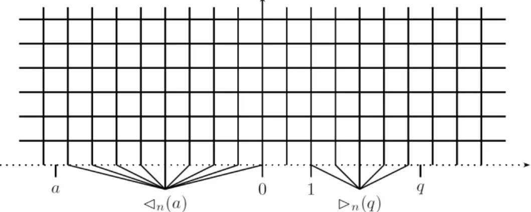
Next we return to the metric graph half-planeeHn. Leta >0. LetGen,a(q) be the metric graph obtained
fromeHn by identifying the following vertices:
• All the vertices in ((n1Z)∩[−a,0])× {0}are identified into a single vertexCn(a).
• All the vertices in ((n1Z)∩[1, q])× {0} are identified into a single vertexBn(q).
See Figure 3. We consider a finite value ofajust to have a finite degree for the quotient vertexCn(a),
but eventually we will considera→+∞.
Figure 3. Illustration of points identified intoCn(a) andBn(q).
As the length of the line joining (ni,nj) to (i+1n ,nj) or (ni,jn) to (ni,j+1n ) is 1n, the corresponding conductance is according to (2.1) equal to n2. LetCn,aeq(q) be the equivalent (or effective) conductance
between Cn(a) and Bn(q) when all the points in (1n)Z× {0} other than those identified to Cn(a) or Bn(q) have the same electrical potential. According to (2.5),
Cn,aeq (q) =n 2 bnqc X i=n P(i n, 1 n) BeHn hits 1 nZ × {0}on [−a,0]× {0} . Asatends to infinity,Ceq
n,a(q) increases and converges to
(2.6) Cneq(q) =n 2 bnqc X i=n P(i n, 1 n) BeHn hits 1 nZ × {0}on (−∞,0]× {0} .
Lemma 2.2. For alln∈N∗ andq >1,Cneq(q)<+∞. Moreover,
lim n→+∞ 1 nC eq n (q) = 1 8πlog(q).
Proof. Using the computation (1.5) and the asymptotic expansion (1.6), we get that Cneq(q)<+∞and that 1 nC eq n (q) = 1 8π bnqc X i=n +∞ X j=0 1 (i+j)2+O bnqc X i=n +∞ X j=0 1 (i+j)3 = 1 8π bnqc X i=n 1 i +O bnqc X i=n 1 i2 = 1 8πlog(q) +O 1 n . Let νeHn
exc([−a,0]) be the measure on excursions νeexcHn((−∞,0]) restricted to the excursions from and to [−a,0]× {0}. LetLGen,a(q)
α be the loop-soup associated to the Brownian motion on the metric graph
e
Gn,a(q), killed at the first hitting time of (1n)Z× {0}outside the points identified toCn(a) orBn(q). Let
(Lbzn,a,q,α)z∈ e
Gn,a(q) be the occupation field of L
e
Gn,a(q)
α . LetNα(Cn(a),Bn(q)) be the number of loops in
LGen,a(q)
α joiningCn(a) toBn(q).
Lemma 2.3. Let a, α, u, v >0. We consider LGen,a(q)
α conditioned on
b
LCn(a)
n,a,q,α=u,LbBn,a,q,αn(q) =v andNα(Cn(a),Bn(q)) = 0.
ThenLGen,a(q)
α consists of three independent families of loops:
• The loops that visit neitherCn(a) norBn(q). These are the same as the loops inLeHαn.
• The loops that visitCn(a). The excursions these loops make outsideCn(a)form a Poisson point
process of intensity 8nπuνeHn
exc([−a,0]).
• The loops that visitBn(q). The excursions these loops make outsideBn(q)form a Poisson point
process of intensity 8nπvνeHn
exc([1, q]).
Proof. This follows from universal properties of loop-soups. The subset of loops that do not visit a given setF0 is distributed like the loop-soup of the same Markov process, but with additional killing at hitting F0 (restriction property). The loops that visit a particular point z can be represented by a Poisson point process of Markovian excursions outsidez. See for instance [3], Sections 2.2, 2.3, 7.1, 7.2, 7.3, and [7], Propositions 9.3.1 and 9.4.1. The factor 8nπ in 8nπuνeHn
exc([−a,0]) and
n
8πvν
eHn
exc([1, q]) comes from the normalisation factor 8π
n in the definition ofν
eHn
exc([−a,0]) ((1.3)) andνeexcHn([1, q]) ((1.4)).
Proposition 2.4. Let u, v >0,q >1 andn≥1.
(2.7) peHn 1/2,u,v(q) = 1−e −2Ceq n(q) 8π√uv n . (2.8) lim n→+∞p eHn 1/2,u,v(q) = 1−q −2√uv.
Proof. Leta >0. Consider three independent Poisson point processes:
• a loop-soupLeHn
1/2,
• a P.p.p of excursions of intensityuνeHn
exc([−a,0]),
• a P.p.p of excursions of intensityvνeHn
exc([1, q]).
The probability for the two P.p.p. of excursions to be connected either directly or through a cluster of
LeHn
1/2 equals, according to Lemma 2.3, the probability forCn(a) andBn(q) to be in the same cluster of
LGen,a(q) 1/2 conditional on LbCn (a) n,a,q,1/2 = 8π nu, LbBn (q) n,a,q,1/2 = 8π
nv and N1/2(Cn(a),Bn(q)) = 0. According to
Lemma 2.1 this probability equals
1−e−2Ceqn,a(q) 8π√uv
n .
Taking the limit asatends to infinity we get (2.7). Using Lemma 2.2 we get the limit (2.8). 3. Computations on continuum half-plane
On the continuum upper half planeHwe consider two independent Poisson point processes:
• a Brownian loop-soupLH
α, 0< α≤1/2,
• a P.p.p. of Brownian excursions from and to (−∞,0]× {0},EH
u((−∞,0]),u >0.
We will consider the clusters made out of loops in LH
α and excursions in EuH((−∞,0]). Among these
clusters we only take the clusters that contain at least one excursion and consider the rightmost envelop of these clusters. This envelop is a non self-intersecting curve joining Rto infinity. It can be formally defined as follows. Take the clusters that contain at least one excursion. The curve minus its starting point onR is the right-most component of the boundary in H of the closure inH of the set of points
visited by the above clusters. All the excursionsEH
u((−∞,0]) are located left to the curve and there are only clusters made of loops
right to it. According to [16] and [19] this boundary curve is an SLE(κ, ρ) starting from 0, where κis given by (1.2) andρby u=(ρ+ 2)(ρ+ 6−κ) 4κ . We will define (3.1) u0(α) := 6−κ(α) 2κ(α) .
We will consider the particular caseu=u0(α) (and thusρ= 0), which is simpler to deal with. SLE(κ, ρ) is then a chordal SLEκcurve starting from 0. For a description of SLE processes see [17]. We will denote
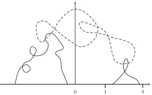
by (ξt)t≥0 this curve. ξ0= 0. It does not touchRat positive times. See Figure 4.
There is only one conformal mapgt that sendsH\ξ([0, t]) (half-plane minus the curve up to timet)
ontoHand that is normalised at infinityz→ ∞as gt(z) =z+
at
z +o(z
−1). 9
Figure 4. Full lines represent Brownian excursions inEH
u((−∞,0]). Dashed lines
rep-resent contours inFext(LH
α). The dotted line representsξ.
Moreover, one parametrises the curve by half-plane capacity (at= 2t). The Loewner flow (gt)t≥0satisfies the differential equation
∂gt(z) ∂t = 2 gt(z)− √ κWt , where (Wt)t≥0 is a standard Brownian motion onR.
Lemma 3.1. Let α ∈ (0,1/2]. pH
α,u0(α),v(q) equals the probability that an excursion from EvH([1, q])
intersects an independent SLEκ(α) curve.
Proof. Letξbe the SLEκ(α)curve constructed fromLHαandEu0H(α)((−∞,0]), independent fromEvH([1, q]).
If no excursion from EH
v([1, q]) intersects ξ, then these excursions are all on the right side of ξ and by
definition ofξ, can only intersects loops inLH
αthat are not connected toEuH0(α)((−∞,0]).
Conversely, assume that an excursion γ from EH
v([1, q]) intersectsξ at a point z0. Then =(z0)>0.
SinceEH
v([1, q]) andξare independent, by the properties of sample Brownian paths, there isε >0 small
enough such that γ makes a closed loop around the disc with center z0 and radius ε, disconnecting it from infinity. Thus, any connected set that intersects both this disc and the real line, has to intersectγ. By the definition ofξ, there is either an excursion fromEH
u0(α)((−∞,0]), or a loop fromL H
αconnected by
a finite chain to an excursion from EH
u0(α)((−∞,0]), that intersects the ε-neighbourhood ofz0. Denote this excursion or loop by γ0. In the first case, the excursion γ0 intersects γ. In the second case, an element from the chain connectingγ0 toEH
u0(α)((−∞,0]) intersectsγ.
The excursions EH
v([1, q]) satisfy the one-sided conformal restriction property (see [18], Section 8,
and [18], Section 4, in particular Section 4.3 ): if K is a compact subset of C that does not intersect
[1, q]× {0} and such that H\K is simply connected, iff is a conformal map from H\K ontoHsuch
thatf(1)< f(q)∈R, then the probability thatEvH([1, q]) does not intersectK equals
f0(1)f0(q)(q−1)2 (f(q)−f(1))2
v . Moreover, conditional on this event, the law of f(EH
v([1, q])) is EvH([f(1), f(q)]), up to a change of
parametrisation of the excursions. From this conformal restriction property, it immediately follows:
Lemma 3.2. Let κ∈(0,4]. Let (ξt)t≥0 be an SLEκ with the driving Brownian motion(
√
κWt)t≥0 and Loewner flow(gt)t≥0. Denote by g0t the derivative ofgtwith respect the complex variable:
g0t(z) = ∂gt(z) ∂z .
Denote byp¯κ,v(q)the probability that an independent family of excursionsEvH([1, q])does not intersectξ.
Then the conditional probability of the event thatEH
v([1, q])does not intersectξconditional on(ξs)0≤s≤t
(or equivalently conditional on(Ws)0≤s≤t) and on not intersecting(ξs)0≤s≤t equals (3.2) p¯κ,v g t(q)− √ κWt gt(1)− √ κWt . The conditional probability of the event that EH
v([1, q])does not intersect ξ conditional on(ξs)0≤s≤tis
(3.3) g0 t(1)gt0(q)(q−1)2 (gt(q)−gt(1))2 v ¯ pκ,v g t(q)− √ κWt gt(1)− √ κWt . In particular, for all t≥0,
(3.4) p¯κ,v(q) =E g0 t(1)gt0(q)(q−1)2 (gt(q)−gt(1))2 v ¯ pκ,v g t(q)− √ κWt gt(1)− √ κWt . Proof. (3.2) is the conditional probability thatgt(EvH([1, q])) does not intersect
(gt(ξt+s))s≥0. To express it we used the fact thatgt(EvH([1, q])) has same law as
EH
v([gt(1), gt(q)]) and that (gt(ξt+s))s≥0 is a chordal SLEκ starting from
√
κWt. In (3.3) we multiplied
the conditional probability that EH
v([1, q]) does not intersect (ξs)0≤s≤t and the conditional probability
thatgt(EvH([1, q])) does not intersect (gt(ξt+s))s≥0.
Next we derive the differential equation inqsatisfied by ¯pκ,v(q) on (1,+∞), provided ¯pκ,visC2-regular. Lemma 3.3. Let κ∈(0,4],v >0 andq >1. Let f be a bounded, C2 function on(1,+∞). Then
g0 t(1)g0t(q)(q−1)2 (gt(q)−gt(1))2 v f g t(q)− √ κWt gt(1)− √ κWt
is a martingale if and only iff satisfies the differential equation
(3.5) f00+ 1 (q−1)q 2− 4 κ q− 4 κ f0− 4v κq2f = 0. Proof. Let (3.6) Rt:= g0t(1)gt0(q)(q−1)2 (gt(q)−gt(1))2 , qt:= gt(q)− √ κWt gt(1)− √ κWt . Rt has bounded variation (int). Let
Mt:=Rvtf(qt).
We apply Itˆo’s formula to (Mt)t≥0.
dMt=Rvt vf(qt) dRt Rt +f0(qt)dqt+ 1 2f 00(q t)dhqit . DenoteH:={=(z)≥0}. Forz∈H\ξ([0, t]), ∂g0t(z) ∂t = ∂ ∂z ∂g t(z) ∂t = ∂ ∂z 2 gt(z)− √ κWt = −2g 0 t(z) (gt(z)− √ κWt)2 . Thus dRt= −2g0 t(1)gt0(q)(q−1)2 (gt(1)− √ κWt)2(gt(q)−gt(1))2 + −2g 0 t(1)gt0(q)(q−1)2 (gt(q)− √ κWt)2(gt(q)−gt(1))2 + 4g 0 t(1)g0t(q)(q−1)2 (gt(1)− √ κWt)(gt(q)−gt(1))3 + −4g 0 t(1)gt0(q)(q−1)2 (gt(q)− √ κWt)(gt(q)−gt(1))3 dt =−2Rt 1 (gt(1)− √ κWt)2 + 1 (gt(q)− √ κWt)2 − 2 (gt(1)− √ κWt)(gt(q)− √ κWt) dt =−2Rt 1 gt(1)− √ κWt − 1 gt(q)− √ κWt 2 dt =−2Rt (qt−1)2 (gt(q)− √ κWt)2 dt. 11
Further dqt= √ κ −1 gt(1)− √ κWt + gt(q)− √ κWt (gt(1)− √ κWt)2 dWt + 2 (gt(q)− √ κWt)(gt(1)− √ κWt) −2 gt(q)− √ κWt (gt(1)− √ κWt)3 +κ gt(q)−gt(1) (gt(1)− √ κWt)3 dt = √ κ(qt−1)qt gt(q)− √ κWt dWt+ (qt−1)qt (gt(q)− √ κWt)2 ((κ−2)qt−2)dt. dhqit= κ(qt−1)2q2t (gt(q)− √ κWt)2 dt. Finally, dMt=Rvtf 0(q t) √ κ(qt−1)qt gt(q)− √ κWt dWt+ Rvt(qt−1) (gt(q)− √ κWt)2 × ×κ 2(qt−1)q 2 tf 00(q t) +qt((κ−2)qt−2)f0(qt)−2v(qt−1)f(qt) dt. It follows that (Mt)t≥0 is a local martingale (hence a true one,f being bounded) if and only if
κ
2(qt−1)q 2
tf00(qt) +qt((κ−2)qt−2)f0(qt)−2v(qt−1)f(qt)≡0,
which gives the equation (3.5).
(3.5) is the differential equation for ¯pκ,v. However, we do not knowa priori that ¯pκ,v is C2-regular.
The idea is to show that both ¯pκ,vand a solution of (3.5) with right boundary conditions are fixed points
of a contracting operator, and thus coincide. We will do this for the caseκ= 4 which interests us.
Proposition 3.4. Let q >1,v >0. lim n→+∞p eHn 1/2,u0(1/2),v(q) =p H 1/2,u0(1/2),v(q) = 1−q −√v. Proof. By definition pH 1/2,u0(1/2),v(q) = 1−p4¯ ,v(q). According to Proposition 2.4, lim n→+∞p e Hn 1/2,u0(1/2),v(q) = 1−q −2√u0(1/2)v= 1−q− √ v. Letfv(q) :=q− √
v. With κ= 4, the ODE (3.5) becomes
f00+1 qf
0− v
q2f = 0
and it is satisfied byfv. According to Lemma 3.3, (Rvtfv(qt))t≥0 is a martingale (we use the notations (3.6) andκ= 4) for any initial value ofq0. In particular for anyt >0
fv(q0) =E[Rvtfv(qt)].
The same is true if we replacefv by ¯p4,v((3.4)). Thus,
(3.7) fv(q0)−p4¯,v(q0) =E[Rtv(fv(qt)−p4¯,v(qt))]
for any starting value ofq0∈(1,+∞) andt >0. ¯
p4,v is non-increasing on (1,+∞) with boundary limits
¯
p4,v(1) = 1, p4¯ ,v(+∞) = 0.
Moreover ¯p4,v is continuous. Indeed, let q ∈ (1,+∞). A.s. there is no excursion in EvH([1, q]) with
endpoint (q,0). This means that ¯p4,vis left-continuous atq. Moreover, a.s. there isε >0 such that there
is no excursion inEH
v([1, q+ε) with an endpoint in [q, q+ε)× {0} that intersects an independent SLE4
curve. This implies that ¯p4,v is right-continuous at q. From the continuity of ¯p4,v follows that there is
ˆ q∈(1,+∞) such that |fv(ˆq)−p4¯ ,v(ˆq)|= max q∈(1,+∞) |fv(q)−p4¯ ,v(q)|. 12
Lett >0 and let ˆqbe the initial valueq0 of (qs)s≥0. From (3.7) we get that
|fv(ˆq)−p4¯,v(ˆq)| ≤E[Rtv]|fv(ˆq)−p4¯,v(ˆq)|.
But a.s.Rt<1 andE[Rvt]<1. This implies that
|fv(ˆq)−p¯4,v(ˆq)|= max q∈(1,+∞) |fv(q)−p¯4,v(q)|= 0 and that ¯ p4,v(q)≡q− √ v. 4. Convergence to CLE In this section we prove the convergence results.
LetQl:= (−l, l)×(0, l). LetLαHn∩Ql,T be the loops in LHαn that are contained inQl and do at least
T jumps. Let LQl
α be the Brownian loops in LHα that are contained in Ql. From [2] follows that for
α∈(0,1/2],l >0 andθ∈(16/9,2),Fext(LHn∩Ql,nθ
α ) converges in law to Fext(LQαl). Lemma 4.1. Let α∈(0,1/2]andθ∈(16/9,2). Fext(LHn,nθ
α )converges in law to Fext(LHα).
Proof. Letz1, . . . , zj ∈H. To deduce thatFext(LHn,nθ
α )[z1, . . . , zj] converges in law toFext(LHα)[z1, . . . , zj]
from the result of [2] we need only to show that lim
l→+∞lim infn→+∞P(Contours ofFext(L
Hn,nθ
α )[z1, . . . , zj] contained inQl) = 1.
Letε∈(0,1/2). There isl0>0 such that
P Contours ofFext(LHα)[z1, . . . , zj] contained inQl0
≥1−ε. Denote
∂HQl:= ({−l} ×(0, l])∪({l} ×(0, l])∪([−l, l]× {l}).
There isl1> l0such that
P(∃γ∈ LHα, γ∩Ql0 6=∅, γ∩∂HQl1 6=∅)≤ε. Then lim n→+∞P(Contours ofFext(L Hn∩Ql1,n θ α )[z1, . . . , zj] contained inQl0)
=P(Contours ofFext(LαQl1)[z1, . . . , zj] contained inQl0)
≥P Contours ofFext(LHα)[z1, . . . , zj] contained inQl0
≥1−ε. According to the approximation of [4],
lim n→+∞P(∃γ∈ L Hn,nθ α , γ∩Ql06=∅, γ∩∂HQl1 6=∅) =P(∃γ∈ LHα, γ∩Ql0 =6 ∅, γ∩∂HQl1 6=∅)≤ε. But P(Contours ofFext(LHn,n θ α )[z1, . . . , zj] contained inQl0)≥ P(Contours of Fext(L Hn∩Ql1,n θ α )[z1, . . . , zj] contained inQl0) −P(∃γ∈ LHn,nθ α , γ∩Ql0 6=∅, γ∩∂HQl1 6=∅). Thus, lim inf n→+∞P(Contours ofFext(L Hn,nθ α )[z1, . . . , zj] contained inQl0)≥1−2ε.
From now onθ∈(16/9,2) will be fixed. αwill belong to (0,1/2]. Forz0∈H, we define
δα,n(z0) := max{d(z,Fext(LHn,n θ
α )(z0))|z∈ Fext(LeHαn)(z0)}.
By z ∈ Fext(LeHαn)(z0) we mean that z is a point on the contour Fext(LeHαn)(z0). The random variable δα,n(z0) is defined only whenFext(LHn,n
θ
α )(z0) is defined, which happens with probability converging to
1.
Lemma 4.2. Assume thatFext(LeHn
α )does not converge in law toFext(LHα). Then there is zα,0∈Hsuch
that δα,n(zα,0) does not converge in law to0.
Proof. IfFext(LeHn
α ) does not converge in law toFext(LHα) then by definition there arez1, . . . , zj∈Hsuch
thatFext(LeHαn)[z1, . . . , zj] does not converge in law to
Fext(LH
α)[z1, . . . , zj]. To the contraryFext(LHn,n θ
α )[z1, . . . , zj] does converge in law toFext(LHα)[z1, . . . , zj].
Since each contour ofFext(LHn,nθ
α )[z1, . . . , zj] is surrounded by a contour ofFext(LeHn
α )[z1, . . . , zj], one of
δα,n(zi) must not converge in law to 0.
Letzα,0 be defined by the previous lemma under the non-convergence assumption. The set of points zon the metric graph contained in or surrounded byFext(LeHn
α )(zα,0) and not in the interior surrounded
byFext(LHn,nθ
α )(zα,0), such thatd(z,Fext(LHn,n θ
α )(zα,0)) =δα,n(zα,0)∧1, is non-empty (whenδα,n(zα,0)
is defined). Indeed,Fext(LeHn
α)(zα,0) plus the set of points it surrounds, minus the interior surrounded by
Fext(LHn,nθ
α )(zα,0), is connected and compact. Let Zα,n be a random point taking values in the above
set, for instance the maximum for the lexicographical order.
Lemma 4.3. Assume thatFext(LeHαn)does not converge in law toFext(LHα). Then there is a sub-sequence
of indicesnα,0 such that the joint law of
(Fext(LHnα,0,n θ α,0
α )(zα,0), Zα,nα,0)
has a limit whennα,0→+∞. It is a law on (Fext(LH
α)(zα,0), Zα)
satisfying the property that with positive probability the point Zα is not contained or surrounded by
Fext(LH α)(zα,0).
Proof. δα,n(zα,0) does not converge in law to 0. This means that there is ε >0 and a sub-sequence of indicesn0 such that
(4.1) ∀n0,P(d(Zα,n0,Fext(LHn0,n 0θ
α )(zα,0))≥ε)≥ε.
The sub-sequence of random variables
(Fext(LHn0,n0θ
α )(zα,0), Zα,n0)
is tight. Indeed the first component of the couple converges in law and the second is by definition at distance at most 1 from the first. Thus there is a sub-sequence of indicesnα,0out ofn0 such that there is a convergence in law. Fext(LHnα,0,n
θ α,0
α )(zα,0) converges in lawFext(LHα)(zα,0). LetZα be defined as
the second component of the limit in law of (Fext(LHnα,0,n θ α,0
α )(zα,0), Zα,nα,0). (4.1) implies that
P(d(Zα,Fext(LαH)(zα,0))≥ε)≥ε.
Moreover, a.s.Zαcannot be in the interior surrounded byFext(LHα)(zα,0) becauseZα,nis not surrounded
byFext(LHn,n
θ
α )(zα,0).
From now on (zj)j≥1 will be a fixed everywhere dense sequence inH.
Lemma 4.4. Assume that Fext(LeHn
α) does not converge in law to Fext(LHα). Then there is a family of
sub-sequences of indicesnα,j such that
• nα,0 is given by Lemma 4.3.
• nα,j+1 is a sub-sequence of nα,j.
• The random variable
(Fext(LHnα,j,n
θ α,j
α )[zα,0, z1, . . . , zj], Zα,nα,j)
converges in law as nα,j →+∞ and the limit defines the joint law of
(Fext(LH
α)[zα,0, z1, . . . , zj], Zα).
• The family of joint laws on (Fext(LH
α)[zα,0, z1, . . . , zj], Zα)j≥1 is consistent in the sense that the law on(Fext(LHα)[zα,0, z1, . . . , zj], Zα)induced by the law of
(Fext(LH
α)[zα,0, z1, . . . , zj+1], Zα)is the same as the one given by the convergence. In particular
the law on(Fext(LH
α)(zα,0), Zα)is the one given by Lemma 4.3.
• The family of laws of(Fext(LH
α)[zα,0, z1, . . . , zj], Zα)j≥1uniquely defines a law on(Fext(LHα), Zα).
Proof. The consistency of law follows from the fact that nα,j+1 is a sub-sequence of nα,j. A contour
loop in Fext(LH
α) almost surely surrounds one of thezj points. Thus the fact that a consistent family
of laws on (Fext(LHα)[zα,0, z1, . . . , zj], Zα)j≥1 uniquely defines a law on (Fext(LHα), Zα) follows from the
Kolmogorov extension theorem.
Next we explain how we extractnα,j+1 out ofnα,j. By construction, the sub-sequence
(Fext(L
Hnα,j,nθα,j
α )[zα,0, z1, . . . , zj], Zα,nα,j) converges in law as nα,j → +∞ and defines a joint law on
(Fext(LH
α)[zα,0, z1, . . . , zj], Zα). Moreover we have the convergence in law of Fext(L
Hnα,j,nθα,j
α )(zj+1) to
Fext(LH
α)(zj+1). Thus the sub-sequence (Fext(L
Hnα,j,nθα,j
α )[zα,0, z1, . . . , zj+1], Zα,nα,j) is tight and one can
extract a subset of indicesnα,j+1 such that it converges in law. The limit law is a law on
(Fext(LHα)[zα,0, z1, . . . , zj+1], Zα). Theorem 4.5. Fext(LHn
1/2) andFext(L eHn
1/2)converge in law as n→+∞ toFext(LH1/2), that is to say to a CLE4 on H.
Proof. It is enough to prove the convergence ofFext(LeH1n/2). Indeed we already have the convergence for
Fext(LHn,nθ
1/2 ) and each contour Fext(L
Hn
1/2)(z) lies between the contour Fext(L
Hn,nθ
1/2 )(z) and the contour
Fext(LeHn
1/2)(z).
Assume that Fext(LeHn
1/2) does not converge in law to Fext(LH1/2). Let z1/2,0 be the point defined by Lemma 4.2 and n1/2,j the sub-sequences defined by Lemma 4.4. We also consider the joint law of
(Fext(LH1/2), Z1/2) defined by Lemma 4.4.
For u, v > 0 and q > 1 we consider additional independent Poisson point processes of excursions
EH
u((−∞,0]) and EvH([1, q]). Let A1/2,u,v(q) be the event that is satisfied if either an excursion from
EH
u((−∞,0]) and one from EvH([1, q]) intersect each other or both intersect a common contour from
Fext(LH
1/2). By definition
P(A1/2,u,v(q)) =pH1/2,u,v(q).
LetA+1/2,u,v(q) be the event that is satisfied if one of the following conditions holds:
• An excursion fromEH
u((−∞,0]) and one fromEvH([1, q]) intersect each other.
• An excursion fromEH
u((−∞,0]) and one fromEvH([1, q]) intersect a common contour fromFext(LH1/2).
• An excursion from EH
u((−∞,0]) intersects Fext(LH1/2)(z1/2,0) and an excursion from EvH([1, q])
hits or surroundsZ1/2.
• An excursion from EH
v([1, q]) intersects Fext(LH1/2)(z1/2,0) and an excursion from EuH((−∞,0])
hits or surroundsZ1/2. We claim that
P(A+1/2,u,v(q))>P(A1/2,u,v(q)) =pH1/2,u,v(q).
To see that the strict inequity holds, consider the following:
• Restrict to the event whenZ1/2is not contained or surrounded by the contourFext(LH1/2)(z1/2,0), which has a positive probability.
• LetK by a compact subset of {=(z)≥0} that contains Fext(L1H/2)(z1/2,0) and Z1/2, such that
H\Kis simply connected and such thatK intersects the real line on (0,+∞) only.
• Since EH
u((−∞,0]) is independent from (Fext(LH1/2), Z1/2, K), there is a positive probability
that no excursions in EH
u((−∞,0]), except one, hits K, and one excursion hits the contour
Fext(LH
1/2)(z1/2,0) without surroundingZ1/2. Then the pointZ1/2is to the right from the region defined by EH
u((−∞,0]) and the contours in Fext(LH1/2) it intersects. See Figure 4 again for a representation of this region.
• SinceEH
v([1, q]) is independent from (Fext(LH1/2), Z1/2,EuH((−∞,0])), there is a positive
probabil-ity that no excursion from EH
v([1, q]) hits the region defined byEuH((−∞,0])) and the contours
inFext(LH1/2) intersected byEuH((−∞,0])), but one excursion fromEvH([1, q]) surrounds the point
Z1/2, which is to the right from this region.
See Figure 5 for the illustration ofA+1/2,u,v(q)\A1/2,u,v(q).
Letj ≥1. The eventsA1/2,u,v(q, j) respectivelyA
+
1/2,u,v(q, j) are defined similarly to A1/2,u,v(q)
re-spectivelyA+1/2,u,v(q), where the condition ofEH
u((−∞,0]) andEvH([1, q]) intersecting a common contour of
Figure 5. Illustration of A+1/2,u,v(q) where an excursion from EuH((−∞,0]) surrounds
Z1/2 and an excursion fromEvH([1, q]) intersects Fext(LH1/2)(z1/2,0).
Fext(LH
1/2) is replaced by the condition of intersecting a common contour ofFext(LH1/2)[z1/2,0, z1, . . . , zj].
Then
lim
j→+∞P(A1/2,u,v(q, j)) =P(A1/2,u,v(q)), j→lim+∞P(A
+
1/2,u,v(q, j)) =P(A
+
1/2,u,v(q)).
We will denote byAn1/2,u,v(q, j) andAn,1/+2,u,v(q, j) the events defined similarly to A1/2,u,v(q, j) andA+1/2,u,v(q, j) by doing the following replacements:
• EH
u((−∞,0]) replaced byEueHn((−∞,0]) andEvH([1, q]) replaced byEveHn([1, q]),
• Z1/2 replaced byZ1/2,n,
• Fext(LH1/2) replaced byFext(LHn
,nθ
1/2 ) andFext(LH1/2)[z1/2,0, z1, . . . , zj] replaced by
Fext(LHn,nθ
1/2 )[z1/2,0, z1, . . . , zj].
Fext(LHn,nθ
1/2 )[z1/2,0, z1, . . . , zn] converges in law to Fext(LH1/2)[z1/2,0, z1, . . . , zj], the P.p.p. EeuHn((−∞,0])
to EH
u((−∞,0]) andEveHn([1, q]) toEvH([1, q]). Moreover, in the limit, if an excursion intersects a contour
loop in Fext(LH
1/2)[z1/2,0, z1, . . . , zj], then a.s. it goes inside the interior surrounded by the loop. Thus
the intersection still holds for small deformations of the excursion and of the contour. Thus for allj≥1 we have the convergence
lim
n→+∞P(A
n
1/2,u,v(q, j)) =P(A1/2,u,v(q, j)).
From Lemma 4.4 follows that lim
n1/2,j→+∞
P(An1/1/22,u,v,j,+(q, j)) =P(A
+
1/2,u,v(q, j)).
Each contour ofFext(LHn
,nθ
1/2 ) is surrounded by a contour ofFext(L1eHn/2) andZ1/2,nbelongs to or is
sur-rounded byFext(LeHn
1/2)(z1/2,0). Thus, on the eventA
n,+
1/2,u,v(q, j), an excursion fromE
e
Hn
u ((−∞,0]) and one
fromEeHn
v ([1, q]) either intersect each other or intersect a common contour fromFext(L
e Hn 1/2)[z1/2,0, z1, . . . , zj]. Thus, peHn 1/2,u,v(q)≥P(A n,+ 1/2,u,v(q, j)).
Letube equal tou0(1/2). Then pH 1/2,u0(1/2),v(q) =n lim 1/2,j→+∞ peHn1/2,j 1/2,u0(1/2),v(q)≥ lim n1/2,j→+∞P (An1/2,j,+ 1/2,u0(1/2),v(q, j)) =P(A + 1/2,u0(1/2),v(q, j)). 16
Taking the limit asj→+∞we get pH 1/2,u0(1/2),v(q)≥j→lim+∞P(A + 1/2,u0(1/2),v(q, j)) =P(A + 1/2,u0(1/2),v(q))> P(A1/2,u0(1/2),v(q)) =p H 1/2,u0(1/2),v(q),
which is a contradiction. It follows thatFext(LeHn
1/2) converges in law to Fext(LH1/2).
Lemma 4.6. Let α∈(0,1/2). Letα¯:= 1/2−α. LetLH
α andLHα¯ be independent and let
LH
1/2=LHα∪ LHα¯.
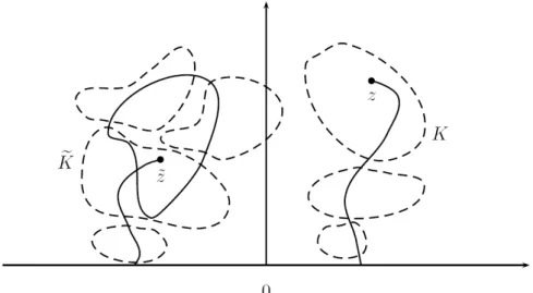
Let z6= ˜z∈H. LetFext• (LHα¯)(˜z), respectivelyFext• (LHα)(z), denote the region surrounded byFext(LHα¯)(˜z), respectively Fext(LH
α)(z), i.e. the complement in H of the unique unbounded connected component of
H\ Fext(LHα¯)(˜z), respectivelyH\ Fext(LHα)(z). The conditional probability
P(Fext(LH1/2)(z)6=Fext(LH1/2)(˜z)|Fext(LHα),Fext(LHα¯)(˜z)) is a.s. positive on the event
Fext• (LHα¯)(˜z)∩ Fext• (LHα)(z) =∅.
Proof. On the event thatFext(LH
α)(z) does not surround ˜zone can choose a continuous path ˜ηjoining ˜zto
∂H=R× {0}and avoidingFext(LHα)(z) (˜ηis thus random and measurable with respect toFext(LHα)(z)).
Let Ke be the union of ˜η, Fext(LαH¯)(˜z) and all the contours in Fext(LHα) that do intersect either ˜η or
Fext(LH
¯
α)(˜z). Let Hull(K) be the hull ofe K, that is to say the complement ine Hof the unique unbounded connected component ofH\K.e
On the event that F•
ext(LHα)(z) does not intersect Fext• (LHα¯)(˜z), z does not belong to Hull(K). Onee can than choose a path η that connects zto ∂Hand avoids Hull(K),e η being random measurable with respect to Hull(K). Lete K be the union of η and all the contours in Fext(LHα) that intersectsη. Let Hull(K) be the hull of K. Figure 6 is an illustration of ˜η,η,Ke andK.
Figure 6. Illustration of ˜η,η, Ke and K. ˜η, η andFext(LHα¯)(˜z) are drawn in full lines. Elements ofFext(LH
α) are drawn in dashed lines.
By construction, on the event
Fext• (LH ¯ α)(˜z)∩ F • ext(LHα)(z) =∅, we have • Hull(K)∩Hull(K) =e ∅,
• H\(Hull(K)∪Hull(K)) is simply connected,e
• no Brownian loop from LH
α crosses the boundary of Hull(K) or Hull(K) and in particular ae contour inFext(LH
α) is either inside Hull(K), Hull(K) or inside the complemente H\(Hull(K)∪ Hull(K)).e
Conditional on Fext• (LH ¯ α)(˜z)∩ F • ext(LHα)(z) =∅,
and on Hull(K), Hull(K), the law of the contourse Fext(LH
\(Hull(K)∪Hull(Ke))
1/2 ), created by the loops
LH\(Hull(K)∪Hull(Ke))
1/2 fromLH1/2that stay insideH\(Hull(K)∪Hull(K)), is a CLEe 4insideH\(Hull(K)∪
Hull(K)), and they are conditionally independent frome LH1/2\ LH
\(Hull(K)∪Hull(Ke)) 1/2 . Conditional on the event
Fext• (LHα¯)(˜z)∩ Fext• (LHα)(z) =∅
and on Hull(K), Hull(K),e Fext(LHα),Fext(LHα¯)(˜z), the probability that
Fext(LH
1/2)(z) =Fext(LH1/2)(˜z)
is less or equal to the probability that Hull(K) and Hull(K) are connected by a cluster ofe LH1/2, which is less or equal to the probability that given the contoursFext(LH\(Hull(K)∪Hull(Ke))
1/2 ) and an independent loop-soup inHof parameter ¯α, there is a contour Γ and two loopsγ1andγ2in the loop-soup of intensity
¯
αsuch that
• γ1intersects Γ and Hull(K),
• γ2intersects Γ and Hull(K).e
The latter conditional probability is a.s. strictly smaller than 1. This is what we needed to prove.
Theorem 4.7. Let α∈ (0,1/2). Fext(LHn
α ) and Fext(LeHαn) converge in law as n→ +∞ to Fext(LHα),
that is to say to a CLEκ(α) on H.
Proof. As for Theorem 4.5, it is enough to prove that Fext(LeHn
α ) converges in law to Fext(LHα). Let us
assume that this is not the case. Letzα,0be the point andnα,0the sub-sequence defined by Lemma 4.2. We also consider the joint law of (Fext(LHα), Zα) defined by Lemma 4.4.
Since lim z→∞P Fext(L H α)(zα,0) =Fext(LHα)(z) = 0 and P d(Zα,Fext(LHα)(zα,0))>0 >0, we can choose ˜z∈Hsuch that
P Fext(LHα)(zα,0) =Fext(LHα)(˜z)
<P d(Zα,Fext(LHα)(zα,0))>0.
In that way
P d(Zα,Fext(LαH)(zα,0))>0,Fext(LHα)(zα,0)=6 Fext(LHα)(˜z)
>0. Let ¯α:= 1/2−α. We takeLH
¯
α independent from (LHα, Zα) andLαeH¯n independent from (LeHαn, Zα,n). We
defineLH
1/2andL eHn
1/2as unions of two independent Poisson point processes:
LH 1/2=LHα∪ LHα¯, L e Hn 1/2=L e Hn α ∪ L eHn ¯ α.
LetAαbe the event defined byFext(LH1/2)(zα,0) =Fext(LH1/2)(˜z). LetA+α be the event which holds if
one of the below conditions is satisfied:
• Fext(LH
1/2)(zα,0) =Fext(LH1/2)(˜z),
• Fext(LHα¯)(˜z) surroundsZα.
Figure 7 is an illustration ofA+
α\Aα.
Let us show thatP(A+
α \Aα)>0. LetE4 be the event defined by the following four conditions:
• d(Zα,Fext(LHα)(zα,0))>0, • Fext(LHα)(zα,0)6=Fext(LHα)(˜z), • Fext(LH ¯ α)(˜z) surroundsZα, • F• ext(LHα¯)(˜z)∩ Fext• (LHα)(zα,0) =∅.
It has positive probability because of our choice of ˜zand the independence ofFext(LH
¯
α)(˜z) from (Fext(LHα), Zα).
Let ¯Aα be the complement ofAα. ¯Aα andE4 are independent conditional on (Fext(LHα),Fext(LHα¯)(˜z)). Thus
P(A+α\Aα) =P(E4,A¯α) =E[1E4P( ¯Aα|Fext(LHα),Fext(LHα¯)(˜z))]. 18
Figure 7. Illustration ofA+α\Aα.
According to Lemma 4.6,P( ¯Aα|Fext(LHα),Fext(LHα¯)(˜z)) is a.s. positive on the event E4. It follows that
P(A+α\Aα)>0.
LetAnα andAn,α+ be the events defined similarly toAα andA+α where the contours Fext(LH1/2)(zα,0),
Fext(LH1/2)(˜z) andFext(LHα¯)(˜z) are replaced by
Fext(LeH1n/2)(zα,0),Fext(LeH1n/2)(˜z) andFext(LeHα¯n)(˜z) respectively andZα is replaced byZα,n. SinceZα,n is
on the contourFext(LeHαn)(zα,0) we have the equalityAn,α+=Anα. From Theorem 4.5 follows that
lim
n→+∞P(A
n
α) =P(Aα).
On the other hand
lim inf nα,0→+∞P (Anα,0,+ α )≥P(A + α)>P(Aα),
which is a contradiction. It follows thatFext(LeHαn) converges in law to Fext(LHα). Acknowledgements
This research was supported by Universit´e Paris-Sud, Orsay.
The author thanks Wendelin Werner for explaining the theory of restriction measures and pointing out the 1/2 factor in the relation between the loop-soup intensity parameter and the central charge.
References
[1] J. Aru, A. Sep´ulveda, and W. Werner. On bounded-type thin local sets of the two-dimensional Gaussian free field.
J. Inst. Math. Jussieu:1–28, 2017.
[2] T. Van de Brug, F. Camia, and M. Lis. Random walk loop soups and conformal loop ensembles.Probab. Theory Related Fields, 166:553–584, 2016.
[3] Y. Le Jan. Markov paths, loops and fields. In2008 St-Flour summer school, L.N. Math., volume 2026. Springer, 2011.
[4] G. F. Lawler and J. A. Trujillo-Ferreras. Random walk loop soup.Trans. Amer. Math. Soc., 359(2):767–787, 2007. [5] G. F. Lawler and W. Werner. The Brownian loop-soup.Probab. Theory Related Fields, 128:565–588, 2004. [6] G.F. Lawler. Partition functions, loop measure, and versions of SLE.J. Stat. Phys., 134:813–837, 2009.
[7] G.F. Lawler and V. Limic. Random walk: a modern introduction, volume 123 ofCambridge Stud. Adv. Math.
Cambridge University Press, 1st edition, 2010.
[8] Y. Le Jan, M.B. Marcus, and J. Rosen. Permanental fields, loop soups and continuous additive functionals.Ann. Probab., 43(1):44–84, 2015.
[9] T. Lupu. From loop clusters and random interlacements to the free field.Ann. Probab., 44(3):2117–2146, 2016. [10] T. Lupu. Loop percolation on discrete half-plane.Electron. Commun. Probab., 21(30), 2016.
[11] J. Miller and S. Sheffield. CLE(4) and the Gaussian free field. In preparation.
[12] O. Schramm and S. Sheffield. Contour lines of the two-dimensional discrete Gaussian free field.Acta Math., 202:21– 137, 2009.
[13] O. Schramm and S. Sheffield. A contour line of the continuum Gaussian free field.Probab. Theory Related Fields, 157:47–80, 2013.
[14] S. Sheffield and W. Werner. Conformal loop ensembles: the Markovian characterization and the loop-soup construc-tion.Ann. of Math., 176(3):1827–1917, 2012.
[15] M. Wang and H. Wu. Level lines of Gaussian free field I: zero-boundary GFF.Stochastic Process. Appl., 127(4):1045– 1124 , 2017.
[16] W. Werner. SLEs as boundaries of clusters of Brownian loops.C.R. Acad. Sci. Paris, 337:481–486, 2003.
[17] W. Werner. Random planar curves and Schramm-Loewner Evolutions. In2002 St-Flour summer school, L.N. Math., volume 1840. Springer, 2004.
[18] W. Werner. Conformal restriction and related questions.Probab. Surv., 2:145–190, 2005. [19] W. Werner and H. Wu. From CLE(κ) to SLE(κ, ρ)’s.Electron. J. Probab., 18:1–20, 2013.
![Figure 4. Full lines represent Brownian excursions in E u H ((−∞, 0]). Dashed lines rep- rep-resent contours in F ext (L H α )](https://thumb-us.123doks.com/thumbv2/123dok_us/9331255.2811609/11.892.159.742.113.378/figure-lines-represent-brownian-excursions-dashed-resent-contours.webp)
![Figure 5. Illustration of A + 1/2,u,v (q) where an excursion from E u H ((−∞, 0]) surrounds Z 1/2 and an excursion from E v H ([1, q]) intersects F ext (L H 1/2 )(z 1/2,0 ).](https://thumb-us.123doks.com/thumbv2/123dok_us/9331255.2811609/17.892.201.706.127.389/figure-illustration-excursion-e-surrounds-excursion-intersects-ext.webp)