Early warning indicators of banking crises: exploring new data and tools 1

(1)

Early warning indicators of banking crises:

exploring new data and tools

1

António Antunes2 _{| Diana Bon}_fi_m3_{| Nuno Monteiro}4_{| Paulo M. M. Rodrigues}5

abstract

Forecasting rare events is a challenge, espe-cially if these events are driven by many

dif-ferent factors and assume diﬀ erent

characte-ristics. We explore the dynamic dimension of discrete choice models to improve the

fore-casting accuracy of early warning models of systemic banking crises. Our results show that introducing this dynamic component into the

models signifi cantly improves the quality of the

results.

1. Introduction

Is it possible to predict the next banking crisis? Almost certainly not. On the one hand, it may be argued that it is econometrically very challenging to predict these very rare events, which in

many cases have diﬀ erent causes and consequences. On the other hand, if accurately predicting

an emerging banking crisis with some anticipation were feasible, policymakers would ideally be able to take all the necessary measures to avoid its materialization, which would then make the method fail.

The aim of this paper is to contribute to improve the early warning toolkit available to policyma-kers. Over the last decades, there have been many and diverse contributions to this literature to

help understand the main drivers of fi nancial crises, as well as to aid policymakers in forecasting

the next crisis. A large part of this literature focuses on currency crises, most notably in emerging market economies (Krugman, 1979, Obstfeld, 1986, Burnside et al., 2004, Chang and Velasco, 2001). Nevertheless, currency crises frequently go hand in hand with banking crises, as noted

by Kaminsky and Reinhart (1999). When a fi nancial crisis is characterized by serious disruptions

and losses in the banking system, the negative eﬀ ects on the economy usually last longer and are

more pronounced (Cecchetti et al., 2009, Jordà et al, 2010, 2012).

Though every crisis seems diﬀ erent and unique (Reinhart and Rogoﬀ , 2011), we explore the

com-monalities in a dataset of European systemic banking crises. Our main contribution relies on exploring the dynamics embedded in the time series of the dependent and independent

varia-bles. We fi nd that using a dynamic probit specifi cation contributes to improve the forecast

accu-racy of early warning models, both in and out of sample.

This paper is organized as follows. In section 2 we describe the data and introduce the models and the estimation methodology used. In section 3 we discuss our main results, analyze the forecasting accuracy of the models and perform robustness checks. Finally, in section 4 we

(2)

2. Data and methodology

2.1. Data

This article was initially developed as a contribution to the ECB Workshop on Early Warning Tools and Tools for Supporting Macroprudential Policies. As described in Alessi et al. (2014), in this workshop a common set of rules and data were given to all participants. The participants were free to use additional data sources, as long as they were publicly available. Furthermore, the variables contained in the dataset could be rescaled or used to create new variables. The only

constraint in this domain was that trend and fi lter calculations could only consider real-time data,

in order to replicate as closely as possible the data available to policymakers in each moment of time. This implies, for instance, using lags of variables to consider the period until data is released

or computing one-sided or recursive trend fi lters.6

Though participants were able to use diﬀ erent methodologies and data sources, the list of

syste-mic banking crises episodes was common, in order to ensure the comparability of results. Indeed,

as noted by Chaudron and de Haan (2014), there are sizeable diﬀ erences across the databases

of systemic banking crises publicly available. Furthermore, Boyd et al. (2009) argue that in many

cases crisis dates refl ect government actions undertaken in response to bank distress and not

the emergence of distress in itself. To ensure the best quality possible for this critical variable, the systemic banking crises database collected by the Czech National Bank (Babecky et al., 2012) was

used. This database benefi ted from the inputs of the Heads of Research of the Eurosystem. The

database was recently updated with contributions from the ESRB/IWG Expert Group (for further

details, see Detken et al., 2014). This database considers two diﬀ erent defi nitions of crises: one

with actual banking crises and another which also includes episodes of heightened vulnerability

which could, ex-post, have justifi ed the implementation of macroprudential tools, even if no crisis

eﬀ ectively occurred.7_{While for the exercise presented at the ECB Workshop on Early Warning}

Tools and Tools for Supporting Macroprudential Policies the former defi nition was considered, in

this paper we use the broader crisis defi nition.

In the abovementioned workshop there was a horse race between diﬀ erent methodologies, as

discussed in Alessi et al. (2014). To allow for the comparability of the results achieved with diﬀ

e-rent techniques, all participants were asked to report values for a contingency matrix, as well as

for the area under the receiver operating characteristic (AUROC) curves.8

The exercise was performed in three diﬀ erent time windows: total, early and late periods. The

total period comprises the 20 to 4 quarters prior to a crisis, grouping the early and late periods.

The early period, defi ned as 20 to 12 quarters before a crisis, should work better as an early

war-ning tool, giving enough time for policymakers to act. The late period, defi ned as 12 to 4 quarters

before the crisis, explores the information content immediately before the emergence of a crisis, when signals may be stronger and policy action may need to be prompter. A similar reasoning is presented by Oet et al. (2010).

Finally, participants were asked to compare not only the in-sample performance of their metho-dologies, but also the out-of-sample performance. Two exercises were suggested: one excluding

the global fi nancial crisis and the other excluding Denmark, Finland and Sweden, where there was

a systemic banking crisis in the late 1980s/early 1990s.

Besides the banking crises data, the dataset provided also included several macroeconomic and

fi nancial variables from various data sources: private credit (from BIS and from IMF); house prices

(3)

ratio (BIS, ECB and EUROSTAT; calculations performed by the ECB based on the methodology by Drehmann and Juselius, 2012). In addition, several bank variables were available: net interest income (OECD), net pre-tax income (OECD), capital and reserves (OECD, EU), leverage ratio (EU), total assets (EU). We tried to maximize the information set available. For that purpose, in some cases we combined the series from a given source with data from other sources available in the dataset. Most variables are provided on a quarterly basis. The longest series span from 1970Q1 to 2010Q4. Moreover, the results presented in this paper rely on an updated version of the data-set initially provided by the ECB, using Thomson Reuters. When the data sources were not the

same, the series were extended using chain growth rates with data up to 2013Q2.9_{In some cases,}

the series were also extended back to previous periods.

We implemented a few transformations of the variables provided. First, we computed several ratios, such as credit-to-GDP and total assets of the banking system as a percentage of GDP. Second, we computed year-on-year growth rates for most of the variables. Finally, we estimated

deviations from long-term trends, using one-sided Hodrick-Prescott fi lters with diﬀ erent

smoo-thing parameters.10

After these transformations, we obtained 37 possible explanatory variables. In order to select the potentially more relevant variables, we performed an univariate analysis similar to the one

described in Bonfi m and Monteiro (2013), examining the AUROC of each series. In addition, the

availability of information was also considered and the shorter series were not included in this analysis. The best performing variables are equity price indices, the year-on-year growth rate of

the debt-to-service ratio, the credit-to-GDP gap with a smoothing parameter of 400 00011 _{and the}

year-on-year growth rate of house prices.

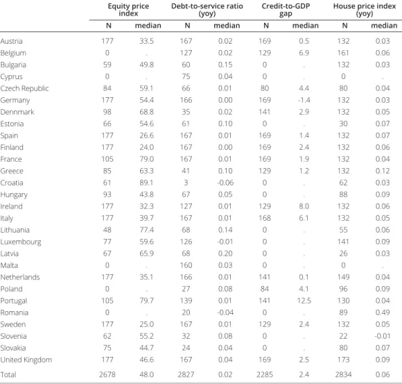
Table 1 presents some descriptive statistics on these variables for the whole sample, while table 2 displays country by country summary statistics. For some countries, there is no information for some of the variables used, thereby implying that these countries are not included in the multiva-riate analysis (Belgium, Bulgaria, Cyprus, Estonia, Croatia, Hungary, Lithuania, Luxembourg, Latvia,

Malta, Poland, Romania, Slovenia and Slovakia). The fi nal sample thus consists of 14 European

countries.

Several features are worth highlighting from table 2. Equity prices reached higher values in Portugal and France and were more subdued in Finland, Sweden and Spain. The highest growth in the debt-to-service ratio was observed in Greece and the UK, while in Germany and Finland this ratio did not change much during most of the sample period. The credit-to-GDP gap, which has been found to be one of the best predictors of banking crises (Drehmann et al., 2010), displays relatively low median values in Germany, Netherlands and Austria. The highest median values for this gap are observed in Portugal, Ireland and Italy. Finally, house prices have increased more

signifi cantly in Greece, UK, Spain, Ireland and Finland. House price dynamics displayed a smaller

magnitude in Germany, Austria, France and Portugal.

2.2. Methodology

Since the seminal work of Estrella and Hardouvelis (1991), binary response models have played an important role in the estimation and forecasting of recessions (see also e.g. Wright, 2006, Kauppi and Saikonnen, 2008, and Nyberg, 2009).

In this paper we consider variants of the general dynamic probit model representation,

* , , 1 1 1 p d p it _k _j kj ij t k _k k i t k it

y

 



 

_ _



x

_





_



y

_



u

(1)

(4)

Table 2 • Summary statistics by country

Equity price

index Debt-to-service ratio (yoy) Credit-to-GDP gap House price index (yoy) N median N median N median N median

Austria 177 33.5 167 0.02 169 0.5 132 0.03 Belgium 0 . 127 0.02 129 6.9 161 0.06 Bulgaria 59 49.8 60 0.15 0 . 132 0.03 Cyprus 0 . 75 0.04 0 . 0 . Czech Republic 84 59.1 66 0.01 80 4.4 80 0.04 Germany 177 54.4 166 0.00 169 -1.4 132 0.03 Dennmark 98 68.8 35 0.02 141 2.9 132 0.05 Estonia 66 54.6 61 0.10 0 . 30 0.07 Spain 177 26.6 167 0.01 169 1.4 132 0.07 Finland 177 24.0 167 0.00 169 2.4 132 0.06 France 105 79.0 167 0.01 169 1.9 132 0.04 Greece 85 63.3 41 0.10 129 1.2 132 0.12 Croatia 61 89.1 3 -0.06 0 . 62 0.03 Hungary 93 43.8 67 0.05 0 . 88 0.09 Ireland 177 32.3 127 0.01 129 8.0 132 0.06 Italy 177 39.7 167 0.01 168 6.1 132 0.05 Lithuania 48 77.4 68 0.14 0 . 55 0.06 Luxembourg 77 59.6 126 -0.01 0 . 141 0.09 Latvia 67 65.9 68 0.20 0 . 26 0.03 Malta 0 . 160 0.03 0 . 0 . Netherlands 177 35.1 166 0.01 141 0.1 149 0.04 Poland 0 . 27 0.08 84 4.1 96 0.09 Portugal 105 79.7 139 0.01 141 12.5 130 0.04 Romania 0 . 20 -0.04 0 . 89 0.49 Sweden 177 25.0 167 0.01 129 2.4 132 0.05 Slovenia 62 55.2 32 0.08 0 . 22 -0.01 Slovakia 75 44.7 24 0.04 0 . 80 0.07 United Kingdom 177 46.6 167 0.04 169 2.5 173 0.09 Total 2678 48.0 2827 0.02 2285 2.4 2834 0.06

Sources: Babecky et al. (2012), BIS, Detken et al. (2014), ECB, Eurostat, IMF, OECD, Thomson Reuters, and authors’ calculations. Note: All variables defi ned in table 1.

Table 1 • Summary statistics

Total sample

N Mean St. dev. Min Median _(p50) Max

Crisis dummy 4816 0.10 0.29 0 0 1

Equity price index 2678 58.5 44.2 1 48.0 265.1

Debt-to-service ratio (yoy) 2827 0.03 0.11 -0.63 0.02 1.24

Credit-to-GDP gap 2285 4.6 12.0 -47.2 2.4 62.5

House price index (yoy) 2834 0.11 0.44 -0.42 0.06 14.42

Sources: Babecky et al. (2012), BIS, Detken et al. (2014), ECB, Eurostat, IMF, OECD, Thomson Reuters, and authors’ calculations.

Notes: yoy - year on year growth rate. The crisis dummy takes the value 1 during banking crises or during periods of heightned vulnerability in which a crisis could be eminent. The equity price index combines data from Eurostat and the IMF, to obtain the longest series possible. The debt-to-service ratio series were provided by the ECB, following the methodology of Drehmann and Juselius (2012). The credit-to-GDP ratio was computed as the ratio between domestic private credit series provided by the BIS (and in some cases extrapolated with IMF data) and nominal GDP. In turn, the credit-to-GDP gap was computed as the deviation from the long-term trend of the credit-to-GDP ratio using a one-sided Hodrick-Prescott fi lter, using a smoothing parameter of 400.000. The house price index combines data from the BIS and OECD.

(5)

where

y

_it is a binary crisis indicator, *

it

y

is a latent variable such that

y

_it



1

if *

0

it

y



and 0

otherwise;

x

_{ij t}_,

,

j



1,...,

p

corresponds to a set of

p

exogenous covariates, and

y

i t k, ,

k=1

,..,

p

corresponds to the

kth

lag of the crisis indicator.

Hence, based on (1), for empirical purposes two distinct models will be considered: i) a marginal

model which results from setting



1

 

...



p



0

, i.e., only considers the eﬀ ects of

covaria-tes on the probability outcomes and treats serial dependence as a nuisance which is captured through association parameters; ii) a transitional model which explicitly incorporates the history

of the response in the regression for *

it

y

(complete model (1)). Hence, in this way, each unit

spe-cifi c history can be used to generate forecasts for that unit, as opposed to the marginal model

which makes forecasts solely on the basis of the values of the exogenous variables.

Estimation of these models is done by maximum likelihood estimation (MLE). The maximization of the likelihood function is a highly nonlinear problem but can be straightforwardly carried out by standard numerical methods. De Jong and Woutersen (2011) showed, for an univariate time series context, that under appropriate regularity conditions, the conventional large sample theory applies to the MLE estimator of the regression parameter vector.

3. Results

3.1 Main results

The fi rst step in the analysis consisted of the estimation of the models previously indicated. Thus,

denoting the endogenous binary response indicator of crisis by yit (taking value 1 if a banking

crisis is observed and zero otherwise), multistep ahead projections can be obtained through the

pooled panel probit specifi cation, where the probability forecast of observing a crisis at time

t

,

it

P y( 1) is given by _{( )}y_it* _{. In particular,}__(.)_{is the Gaussian cumulative distribution function}

and yit

*_{is thus a latent variable. De}_fi_ning

_h

_{as the forecast horizon, we can adjust (1) to produce}

the necessary forecasts, i.e.,

* , , 1 1 1 p d p it _k _j kj ij t k h _k k i t k h it

y

 



 

_ _



x

_{ }





_



y

_{ }



v

₍₂₎

The model was estimated with three diﬀ erent lag structures, as discussed above. First we

con-sidered 20 to 4 lags of all explanatory variables. This allows us to analyse the determinants of banking crisis 1 to 5 years in advance. In addition, we estimated the model in a so-called “early period”, exploring the crisis determinants with a lag between 20 and 12 quarters. This allows us to explore the variables with stronger early warning signals. Finally, we estimate the model in the “late period”, using information lagged between 12 and 4 quarters, thus exploring which variables may be more relevant to signal a crisis in the near future.

For all models, we began by estimating the model with all the lags of the four selected explanatory variables (equity price index, the year-on-year growth rate of the debt-to-service ratio, the credit--to-GDP gap, and the year-on-year-growth rate of the house price index). From that estimation,

we selected only the variables which were statistically signifi cant at a 10% level, thereby

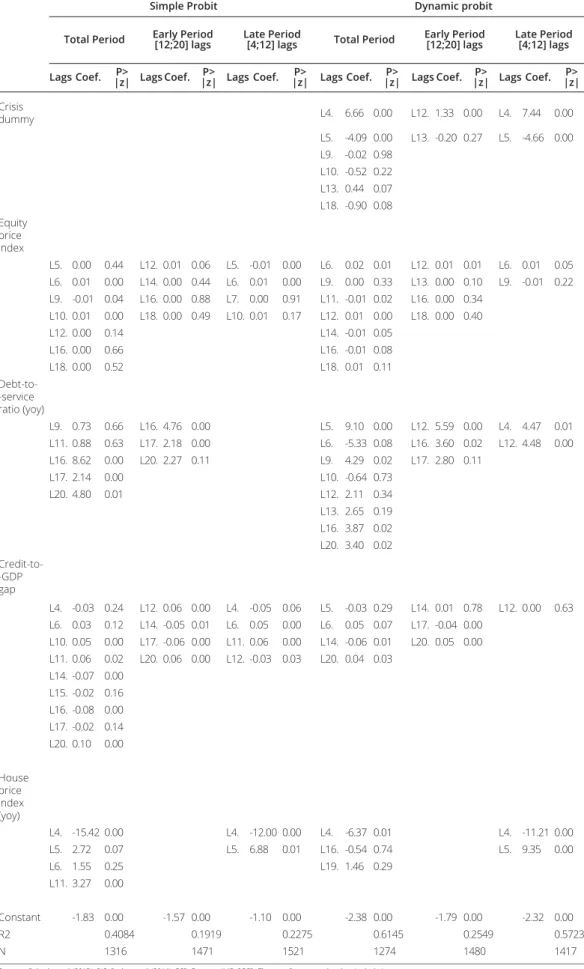
estima-ting a more parsimonious model. These are the results presented in table 3.

The results regarding equity price indices are not remarkably strong. In the parsimonious

repre-sentation, the equity price index provides statistically signifi cant signals (10%) at

t

-6,

t

-9 and

t

-10

quarters. The growth of the debt-to-service ratio provides signals with a signifi cant anticipation

(6)

Table 3 • Regression results: simple and dynamic probits

Simple Probit Dynamic probit

Total Period Early Period _{[12;20] lags} Late Period_{[4;12] lags} Total Period Early Period _{[12;20] lags} Late Period_{[4;12] lags}

Lags Coef. _{|z| Lags Coef.}P> _{|z| Lags Coef.}P> _{|z| Lags Coef.}P> _{|z| Lags Coef.}P> _{|z| Lags Coef.}P> _|z|P>

Crisis dummy L4. 6.66 0.00 L12. 1.33 0.00 L4. 7.44 0.00 L5. -4.09 0.00 L13. -0.20 0.27 L5. -4.66 0.00 L9. -0.02 0.98 L10. -0.52 0.22 L13. 0.44 0.07 L18. -0.90 0.08 Equity price index L5. 0.00 0.44 L12. 0.01 0.06 L5. -0.01 0.00 L6. 0.02 0.01 L12. 0.01 0.01 L6. 0.01 0.05 L6. 0.01 0.00 L14. 0.00 0.44 L6. 0.01 0.00 L9. 0.00 0.33 L13. 0.00 0.10 L9. -0.01 0.22 L9. -0.01 0.04 L16. 0.00 0.88 L7. 0.00 0.91 L11. -0.01 0.02 L16. 0.00 0.34 L10. 0.01 0.00 L18. 0.00 0.49 L10. 0.01 0.17 L12. 0.01 0.00 L18. 0.00 0.40 L12. 0.00 0.14 L14. -0.01 0.05 L16. 0.00 0.66 L16. -0.01 0.08 L18. 0.00 0.52 L18. 0.01 0.11 Debt-to--service ratio (yoy) L9. 0.73 0.66 L16. 4.76 0.00 L5. 9.10 0.00 L12. 5.59 0.00 L4. 4.47 0.01 L11. 0.88 0.63 L17. 2.18 0.00 L6. -5.33 0.08 L16. 3.60 0.02 L12. 4.48 0.00 L16. 8.62 0.00 L20. 2.27 0.11 L9. 4.29 0.02 L17. 2.80 0.11 L17. 2.14 0.00 L10. -0.64 0.73 L20. 4.80 0.01 L12. 2.11 0.34 L13. 2.65 0.19 L16. 3.87 0.02 L20. 3.40 0.02 Credit-to--GDP gap L4. -0.03 0.24 L12. 0.06 0.00 L4. -0.05 0.06 L5. -0.03 0.29 L14. 0.01 0.78 L12. 0.00 0.63 L6. 0.03 0.12 L14. -0.05 0.01 L6. 0.05 0.00 L6. 0.05 0.07 L17. -0.04 0.00 L10. 0.05 0.00 L17. -0.06 0.00 L11. 0.06 0.00 L14. -0.06 0.01 L20. 0.05 0.00 L11. 0.06 0.02 L20. 0.06 0.00 L12. -0.03 0.03 L20. 0.04 0.03 L14. -0.07 0.00 L15. -0.02 0.16 L16. -0.08 0.00 L17. -0.02 0.14 L20. 0.10 0.00 House price index (yoy) L4. -15.42 0.00 L4. -12.00 0.00 L4. -6.37 0.01 L4. -11.21 0.00 L5. 2.72 0.07 L5. 6.88 0.01 L16. -0.54 0.74 L5. 9.35 0.00 L6. 1.55 0.25 L19. 1.46 0.29 L11. 3.27 0.00 Constant -1.83 0.00 -1.57 0.00 -1.10 0.00 -2.38 0.00 -1.79 0.00 -2.32 0.00 R2 0.4084 0.1919 0.2275 0.6145 0.2549 0.5723 N 1316 1471 1521 1274 1480 1417

Sources: Babecky et al. (2012), BIS, Detken et al. (2014), ECB, Eurostat, IMF, OECD, Thomson Reuters, and authors’ calculations.

(7)

credit-to-GDP gap is the variable that displays more statistically signifi cant coeﬃ cients, with

use-ful signals many quarters ahead of crisis. However, the signs of these coeﬃ cients are not always

consistent, i.e., in some quarters the estimated coeﬃ cients are positive, whereas in others they

turn out to be negative. Finally, the year-on-year growth rate of house prices also displays mixed

signals, with a positive coeﬃ cient at

t

-5 and

t

-11, and a perhaps more counterintuitive negative

coeﬃ cient at

t

-4. This may suggest that systemic banking crises are more likely after periods of

strong growth in house prices that are followed by sharp declines.

In the early period (

t

-20 to

t

-12), the results are somewhat diﬀ erent. House prices growth is never

statistically signifi cant, thereby showing that this variable does not have strong early warning

properties in a multivariate setting. Debt-to-service ratio growth appears signifi cant at

t

-16 and

t

-17, maintaining the positive signs of the total period estimation. Equity price indices display a

signifi cant positive signal with a lag of 12 quarters. The credit-to-GDP gap is also signifi cant in

several periods.

In the period closer to the crisis (

t

-12 to

t-

4), the growth of the debt-to-service ratio is never

sta-tistically signifi cant. This means that this variable has strong early warning signalling properties,

though not close to the emergence of a crisis. The other three variables continue to provide signifi cant signals.

In the second part of table 3 we present the results for the dynamic models. As discussed before, by exploring the dynamics embedded in a crises time series, we hope to be able to improve the quality of our early warning model. Indeed, including lagged dependent variables in the model

specifi cation seems to substantially improve the model fi t. Several lags of the dependent

varia-ble turn out to be statistically signifi cant in explaining the likelihood of occurrence of a systemic

banking crisis, in the three diﬀ erent estimation windows considered. The results concerning the

other explanatory variables are broadly consistent. The main exception is the growth of the

debt--to-service ratio, which is now signifi cant also in the late period.

All in all, the growth of debt-to-service ratios seems to provide useful guidance for policymakers

signifi cantly ahead of crises. The credit-to-GDP gap provides strong signals in all horizons, though

not always consistent.

3.2 Model assessment

The main goal of this exercise is to provide useful early warning guidance to policymakers ahead of systemic banking crises. To test how useful the guidance provided by the models may be, seve-ral assessment metrics may be considered.

Since the model is a binary response one, we can defi ne a cut-oﬀ value for the latent variable.

The observation is classifi ed by the model as “crisis” if the latent variable is above the cut-oﬀ ;

otherwise, the observation is “non crisis”. This procedure defi nes, for each cut-oﬀ , a classifi cation

for each observation in the sample. Notice that we know, from the data, the actual classifi cation

of each observation, that is, what actually happened in each country-quarter pair of the sample. Against this background, it is possible to build a contingency matrix that includes four elements: number of true positives (TP - number of correctly predicted crises by the model), number of true negatives (TN – number of non-crises observations correctly predicted by the model), number of false positives (FP) and number of false negatives (FN).

Naturally, a perfect model would classify correctly all observations. This does not happen in

prac-tice. As a matter of fact, a very negative value for the cut-oﬀ means that a lot of non crisis

(8)

can think of as a false alarm). As we increase the cut-oﬀ , more and more non crisis observations

are going to be classifi ed as such by the model but some observations that actually are crisis are

going to be classifi ed as non crisis (this is the type II error, or a “wolf in a sheep’s clothing”). When

the cut-oﬀ is very high, all observations are classifi ed as non crisis – and so all crisis observations

will be wrongly classifi ed as non crisis by the model.

We call specifi city to the fraction of non crisis observations that are correctly classifi ed by the

model, and sensitivity to the fraction of crisis observations that are correctly classifi ed by the

model.

When the cut-oﬀ is minus infi nity, all observations are classifi ed as crisis by the model; therefore,

sensitivity is 1 and specifi city is 0. When the cut-oﬀ is plus infi nity, sensitivity is 0 and specifi city is

1. By varying the cut-oﬀ we obtain a set of values for these two measures. A possible

represen-tation of the model’s performance is the Receiver Operating Characteristic curve (or ROC), which we can see in chart 1. This chart illustrates two hypothetical ROC curves. In the horizontal axis

we represent 1 minus specifi city, that is, the percentage of non crisis observations incorrectly

classifi ed as crisis by the model (i.e., type I errors). In the vertical axis we represent sensitivity, that

is, the fraction of crisis observations correctly classifi ed as crisis by the model. A given point (x,y)

in the curve answers the following question: What percentage x of non crisis observations will be

incorrectly classifi ed by the model in order to classify correctly a percentage y of crisis

observa-tions? In a perfect model we would be able to correctly classify 100 percent of crisis observations without incorrectly classifying any non crisis observation (0 percent). This means that the perfect model’s ROC curve would be the line segment between points (0,1) and (1,1). On the other hand, a model randomly classifying observations will have a ROC curve given by the line segment bet-ween points (0,0) and (1,1), i.e., a 45º degree line. In other words, the model would incorrectly classify 25 percent of the non crisis observations to correctly classify 25 percent of the crisis observations. This fact suggests that an adequate measure for the performance of the model is the area under the ROC curve, commonly known as AUROC.

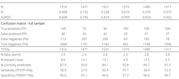
Chart 2 plots the ROC curves for the six specifi cations presented in table 3, while table 4 presents

several indicators to assess the quality of these models.

Examining the model’s goodness of fi t (evaluated using McFadden R2_{) and the AUROC provides}

consistent results. The best performance is always obtained for the total period estimation. In contrast, the early period estimations provide the weakest results. This is not surprising, as it

Se n sit iv ty 1-Specificity 1 1 45º 0 Chart 1 • Examples of ROC curves

(9)

Chart 2 • ROC curves

Simple Probit

Total Period Early Period Late Period

0.00 0.25 0.50 0.75 1.00 Sensitivity 0.00 0.25 0.50 0.75 1.00 1 - Specificity

Area under ROC curve = 0.8983

Dynamic probit

Total Period Early Period Late Period

Sources: Babecky et al. (2012), BIS, Detken et al. (2014), ECB, Eurostat, IMF, OECD, Thomson Reuters, and authors’ calculations.

Table 4 • Model evaluation

Simple Probit Dynamic probit

Total Period Early Period Late Period Total Period Early Period Late Period

N 1316 1471 1521 1274 1480 1417

R2 _0.408 _0.192 _0.228 _0.615 _0.255 _0.572

AUROC 0.898 0.792 0.819 0.959 0.834 0.952

Confusion matrix - full sample

True positives (TP) 149 79 96 190 106 204 False positives (FP) 46 34 42 29 41 37 False negatives (FN) 113 207 200 63 185 78 True negatives (TN) 1008 1151 1183 992 1148 1098 TOTAL 1316 1471 1521 1274 1480 1417 % false alarms 3.5 2.3 2.8 2.3 2.8 2.6 % missed crises 8.6 14.1 13.1 4.9 12.5 5.5 % correctly predicted 87.9 83.6 84.1 92.8 84.7 91.9 Sensitivity (TP/(TP+FN)) 56.9 27.6 32.4 75.1 36.4 72.3 Specifi city (TN/(FP+TN)) 95.6 97.1 96.6 97.2 96.6 96.7

Sources: Babecky et al. (2012), BIS, Detken et al. (2014), ECB, Eurostat, IMF, OECD, Thomson Reuters, and authors’ calculations.

(10)

would be expected that signals are stronger immediately before the crisis than 3 years before. Nevertheless, looking at information for a long period is relevant, as the total period estimation performs better than the late period (12 to 4 quarters before the crisis).

Regarding the methodology, the model’s performance, assessed by the R2_{and the AUROC, is}

substantially better when we include dynamic eﬀ ects, using the lagged dependent variable. This

shows that exploring the dynamics of the dependent variable helps to signifi cantly improve the

performance of the model, in all the estimation horizons considered.

Though the model’s goodness of fi t and the AUROC are useful summary measures to assess

the performance of each model, it is relevant to consider how many crises the model correctly predicts, how many it fails to predict and how many false alarms exist. This is relevant especially in a setting as ours, with potentially relevant implications for decision-making. Indeed, as noted

by Alessi and Detken (2011), policymakers are not indiﬀ erent between missing a crisis or acting

upon false alarms. As there is a trade-oﬀ between these two dimensions, which are subsumed in

the AUROC, it might be relevant to look at them separately.

Dynamic probits are able to reduce the percentage of false alarms only for the total and late period estimations. Nevertheless, this percentage is very small in all the models, being at most

3.5 per cent (simple probit for the total period estimation). In contrast, dynamic probits signifi

-cantly reduce the percentage of missed crises (from 8.6 to 4.9 per cent, in the total period esti-mation). Given that missing a crisis may be costlier than issuing a false alarm (Demirgüç-Kunt and Detragiache, 1999, Borio and Lowe, 2002, and Borio and Drehmann, 2009), this result suggests that dynamic models may be more useful for policymakers. In addition, dynamic models are able to correctly predict a larger percentage of crisis episodes, most notably in the total and late periods.

It is also interesting to see that dynamic probits allow to signifi cantly increase the models’

sensiti-vity. As mentioned above, sensitivity is defi ned as the number of true positives as a percentage of

the total number of crises, thereby being a so-called true positive rate. This confi rms that dynamic

probits are more helpful in identifying crisis periods than marginal models. In turn, the specifi

-city of the model, which is defi ned as the true negatives as a percentage of the total non-crises

periods, decreases slightly in the dynamic models, though remaining very high.

All in all, a large battery of metrics confi rms that adding a dynamic component to early warning

crises models substantially improves the quality of the results, most notably in reducing the per-centage of missed crises and in increasing the perper-centage of those that are correctly predicted.

As discussed in Section 2.1, this methodology was part of a horse race between diﬀ erent

metho-dologies presented in an ECB workshop. As mentioned in Alessi et al. (2014), dynamic probits were amongst the best performing methodologies.

3.3 Robustness

The results presented so far assess the in-sample performance of the model. However, the qua-lity of the model hinges on its forecasting accuracy. It is thus essential to test the model’s

out-of--sample performance. To do that, two diﬀ erent exercises were considered. First, an out-of-period

(11)

countries (we excluded all quarters from 2007Q1 onwards). The second exercise was an out--of-sample estimation, by excluding Denmark, Finland and Sweden, where there was a systemic banking crisis in the late 1980s/early 1990s, from the estimation and testing the accuracy of the model for these countries ex-post.

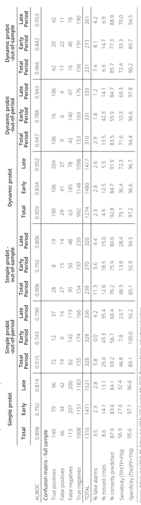
The results of the simple and dynamic models’ performance in these two exercises are presented in table 5. The table shows several evaluation metrics for the simple and dynamic probits, in the three estimation windows considered (total, early and late periods). The in-sample results are compared to the out-of-period and out-of-sample estimations. In these two cases, the models are estimated excluding, respectively, the period and countries mentioned above. The metrics refer to the performance of the prediction of the model for these excluded observations.

We fi nd that the AUROC for the out-of-sample and out-of-period estimations does not decrease

signifi cantly in most of the specifi cations. On the contrary, it actually increases in the simple probit

estimations for the total period, as well as in all the out-of-sample dynamic estimations. In turn,

the AUROC for the out-of-period estimations decreases only slightly, thus confi rming that the

performance of the model does not critically depend on the global fi nancial crisis. This could be

a concern, as a signifi cant part of the crisis observations in diﬀ erent countries is recorded after

2007.

Nevertheless, the percentage of false alarms increases somewhat, most notably in the

out-of--sample estimations. Moreover, the percentage of missed crises increases more signifi cantly in

the out-of-period estimation, thus suggesting that the model would not be able to predict the

glo-bal fi nancial crisis in all the countries in the sample. The percentage of correctly predicted crises

also decreases more in this estimation. These latter results are not unexpected, as this crisis was driven in many countries by exogenous shocks rather than by underlying vulnerabilities.

4. Concluding remarks

Systemic banking crises are rare, yet extremely costly, events. Accurately predicting them is still very challenging, despite the large body of literature in this domain. In this paper, we provide a methodological contribution to this literature, by exploring the role of dynamic probits in predic-ting these events.

Using a comprehensive dataset of systemic banking crisis in Europe, we fi nd that equity prices,

house prices growth, credit-to-GDP gaps and the growth of debt to service ratios are among the most useful indicators in signalling emerging crises. The last two indicators provide the strongest and most consistent signals in a multivariate setting.

We show that adding a dynamic component to the multivariate modelling of systemic banking crises substantially improves the models’ accuracy. This result holds both in and out of sample.

(12)

Table 5 • Out-of-sample and out-of-period estimation

Simple probit

Simple probit -out-of-period Simple probit - out-of-sample

Dynamic probit

Dynamic probit -out-of-period Dynamic probit -out-of-sample

Total Early Late Total Period Early Period Late Period Total Period Early Period Late Period Total Early Late Total Period Early Period Late Period Total Period Early Period Late Period AUROC 0.898 0.792 0.819 0.915 0.743 0.790 0.906 0.792 0.806 0.959 0.834 0.952 0.947 0.788 0.943 0.966 0.842 0.953

Confusion matrix - full sample True positives

14 9 79 96 72 12 37 28 8 19 190 106 204 106 16 106 42 20 42 False positives 46 34 42 19 0 14 27 15 14 29 41 37 9 6 4 17 22 11 False negatives 11 3 20 7 20 0 82 142 119 30 50 48 63 185 78 42 140 47 16 40 18 True negatives 1008 1151 1183 155 174 166 154 197 239 992 1148 1098 153 169 176 156 191 190 TOTAL 1316 1471 1521 328 328 336 239 270 320 1274 1480 1417 310 331 333 231 273 261 % false alarms 3. 5 2. 3 2. 8 5.8 0.0 4.2 11.3 5.6 4.4 2.3 2.8 2.6 2.9 1.8 1.2 7.4 8.1 4.2 % missed crises 8.6 14.1 13.1 25.0 43.3 35.4 12.6 18.5 15.0 4.9 12.5 5.5 13.5 42.3 14.1 6.9 14.7 6.9 % correctly predicted 87.9 83.6 84.1 69.2 56.7 60.4 76.2 75.9 80.6 92.8 84.7 91.9 83.5 55.9 84.7 85.7 77.3 88.9 Sensitivity (TP/(TP+FN)) 56.9 27.6 32.4 46.8 7.8 23.7 48.3 13.8 28.4 75.1 36.4 72.3 71.6 10.3 69.3 72.4 33.3 70.0 Speci fi city (TN/(FP+TN)) 95.6 97.1 96.6 89.1 100.0 92.2 85.1 92.9 94.5 97.2 96.6 96.7 94.4 96.6 97.8 90.2 89.7 94.5 Sources: Babecky et al. (2012), BIS, Detken et al.

(2014), ECB, Eurostat, IMF, OECD, Thomson Reuters, and authors’ calculations.

Notes: the results for the out-of-sample exercise exclude Denmark, Finland and Sweden, where there was a systemic banking cris

is in the late 1980s/early 1990s, and the results for the out-of-period exclude the global

fi

nancial crisis that started in 2007. The total period refers to lags [4;20], the early period [12;20] and

(13)

Notes

1. We are thankful to participants in the ECB/MaRs Workshop on Early Warning Tools and Tools for Supporting Macroprudential Policies and in a seminar

at Banco de Portugal for insightful comments and suggestions. The analyses, opinions and fi ndings of this article represent the views of the authors, which

are not necessarily those of Banco de Portugal.

2. Banco de Portugal, Economics and Research Department and Nova School of Business and Economics. 3. Banco de Portugal, Economics and Research Department.

4. Banco de Portugal, Economics and Research Department.

5. Banco de Portugal, Economics and Research Department and Nova School of Business and Economics.

6. Despite these eﬀ orts, the information is not exactly the same as that that would be available to policymakers, as many macroeconomic variables are

subject to ex-post revisions. Edge and Meisenzahl (2011) show that these diﬀ erences can be sizeable when computing the credit-to-GDP ratio, thereby

leading to potential diﬀ erences when setting macroprudential instruments such as the countercyclical capital buﬀ er ratio.

7. For instance, for Portugal, one additional stress episode that was not eﬀ ectively a crisis, but in which sizeable vulnerabilities were building up was

included. In this period, the occurrence of an endogenous or exogenous shock could have originated an abrupt adjustment of underlying vulnerabilities.

Based on this, the quarters 1999Q1 – 2000Q1 were classifi ed as a stress period. See Bonfi m and Monteiro (2013) for further details.

8. See defi nitions of these concepts in Section 3.2 Model assessment.

9. The only series that was not possible to update was the debt-to-service ratio.

10. For an illustration of the impacts of using diﬀ erent smoothing parameters in a similar setting, please see Bonfi m and Monteiro (2013).

11. According to the Basel Committee (2010) and Drehmann et al. (2010), the deviation of the ratio between credit and GDP from its long term trend is the

indicator that better performs in signaling the need to build up capital before a crisis, when examining several indicators for diﬀ erent countries. Given this

evidence, the Basel Committee (2010) proposes that buﬀ er decisions are anchored on the magnitude of these deviations (though recognizing the need to

complement the decisions with other indicators, as well as with judgment).

REFERENCES

Alessi, L., A. Antunes, J. Babecký, S. Baltussen,

M. Behn, D. Bonfi m, O. Bush, C. Detken, J. Frost,

R. Guimarães, T. Havránek, M. Joy, K. Kauko, J.

Matějů, N. Monteiro, B. Neudorfer, T. Peltonen,

P. M. M. Rodrigues, M. Rusnák, W. Schudel, M. Sigmund, H. Stremmel, K. Šmídková, R. van

Tilburg, B. Vašíček, and D. Žigraiová (2014),

“A Horse Race of Early Warning Systems Developed by the Macroprudential Research Network“, mimeo.

Alessi, L. and C. Detken (2011), “Quasi real time early warning indicators for costly asset price boom/bust cycles: A role for global liquidity“, European Journal of Political Economy, 27(3), 520–533.

Babecky, J., Havranek, T., Mateju, J., Rusnak, M.,

Smidkova, K., and B. Vasicek, (2012), “Banking,

debt and currency crises: early warning

indi-cators for developed countries“, ECB Working

Paper: 1485/2012.

Basel Committee (2010), “Guidance for National Authorities Operating the Countercyclical

Capital Buﬀ er“.

Bonfi m, D. and N. Monteiro (2013), “The

imple-mentation of the countercyclical capital buﬀ er:

rules versus discretion“, Banco de Portugal Financial Stability Report, November 2013. Borio, C. and M. Drehmann (2009), “Assessing the risk of banking crises – revisited“, BIS Quarterly Review, March, pp 29-46.

Borio, C. and P. Lowe (2002), “Assessing the risk of banking crises“, BIS Quarterly Review, pp 43-54.

Boyd, J., De Nicolò G., and E. Loukoianova (2009), “Banking Crises and Crisis Dating: Theory and Evidence“, IMF Working Paper 09/141.

Burnside, C., Eichenbaum M., and S. Rebelo (2004), “Government guarantees and

self-ful-fi lling speculative attacks“, Journal of Economic

(14)

Chang, R. and A. Velasco (2001), “A model of

fi nancial crises in emerging markets“, Quarterly

Journal of Economics, 116, 489-517.

Chaudron, R. and J. de Haan (2014), “Identifying and dating systemic banking crises using inci-dence and size of bank failures“, DNB Working Paper No. 406.

Cecchetti, S., Kohler M., and C. Upper (2009), “Financial Crises and Economic Activity“, NBER Working Paper 15379.

de Jong, R. M. and T. M. Woutersen (2011), “Dynamic Time Series Binary Choice“, Econometric Theory 27, 673 - 702.

Demirgüç-Kunt, A. and E. Detragiache (1999), “Monitoring banking sector fragility: A multi-variate logit approach with an application to the 1996-97 crisis“, World Bank Policy Research Working Paper No. 2085.

Detken, C., Weeken O., Alessi L., D. Bonfi m,

M. M. Boucinha, C. Castro, S. Frontczak, G. Giordana, J. Giese, N. Jahn, J. Kakes, B. Klaus, J. H. Lang, N. Puzanova and P. Welz (2014), “Operationalising the countercyclical capital

buﬀ er: indicator selection, threshold identifi

ca-tion and calibraca-tion opca-tions“, ESRB Occasional Paper, forthcoming.

Drehmann, M., Borio, C., Gambacorta, L., Jimenez, G. and Trucharte, C. (2010), “Countercyclical

Capital Buﬀ ers: Exploring options“, BIS Working

Paper No. 317.

Drehmann, M. and M. Juselius (2012) “Do debt

service costs aﬀ ect macroeconomic and fi

nan-cial stability?”, BIS Quarterly Review, September, pp. 23-25

Edge, R. and R. Meisenzahl, (2011), “The Unreliability of Credit-to-GDP Ratio Gaps in Real Time: Implications for Countercyclical

Capital Buﬀ ers“, International Journal of Central

Banking, December 2011, 261-298.

Estrella A, and G.A. Hardouvelis (1991), “The term structure as a predictor of real economic activity“, Journal of Finance 46, 555–576. Jordà, O., Schularick M., and A. M. Taylor (2010), “Financial crises, credit booms, and exter-nal imbalances: 140 years of lessons“, NBER Working Paper 16567.

Jordà, O., Schularick M., and A. M. Taylor (2012), “When Credit Bites Back: Leverage, Business Cycles, and Crises“, Federal Reserve Bank of San Francisco Working Paper 2011-27.

Kaminsky, G. and C. Reinhart (1999), “The Twin Crises: The Causes of Banking and Balance-of-Payments Problems“, American Economic Review, 89(3), 473-500.

Kauppi, H. and P. Saikkonen (2008), “Predicting U.S. Recessions with Dynamic Binary Response

Models.“, Review of Economics and Statistics

90(4), 777-791.

Krugman, P. (1979), “A Model of Balance-of-Payments Crises“, Journal of Money, Credit and Banking, 11(3), 311-325.

Nyberg, H. (2010), “Dynamic Probit Models and Financial Variables in Recession Forecasting“, Journal of Forecasting 29, 215–230

Obstfeld, M. (1986), “Rational and Self-Fulfi lling

Balance-of-Payments Crises“, American Economic Review, 76(1), 72-81.

Oet, M., R. Eiben, D. Gramlich, G. L .Miller and S. J. Ong (20 10), “SAFE: An Early Warning System for Systemic Banking Risk“, mimeo.

Reinhart, C. and R. Rogoﬀ , (2011), “This Time

Is Diﬀ erent: Eight Centuries of Financial Folly“,

Princeton University Press.

Wright, J.H. (2006), “The yield curve and pre-dicting recessions.“, Finance and Economics Discussion Series no. 7, Board of Governors of the Federal Reserve System.