FORWARD RATE DEPENDENT MARKOVIAN
TRANSFORMATIONS OF THE HEATH-JARROW-MORTON TERM STRUCTURE MODEL
CARL CHIARELLA AND OH KANG KWON
School of Finance and Economics University ofTechnology Sydney
PO Box 123 Broadway NSW 2007
Australia
[email protected] [email protected]
Abstract. In this paper, a class of forward rate dependent Markovian trans-formations of the Heath-Jarrow-Morton [HJM92] term structure model are obtained by considering volatility processes that are solutions of linear ordi-nary differential equations. These transformations generalise the Markovian systems obtained by Carverhill [Car94], Ritchken and Sankarasubramanian [RS95], Bhar and Chiarella [BC97], and Inui and Kijima [IK98], and also gen-eralise the bond price formulae obtained therein.
Introduction
In the risk neutral Heath-Jarrow-Morton [HJM92] term structure model, evo-lution of the forward rate process is completely determined by the forward rate volatilities. The HJM framework is very general and contains many of the ear-lier interest rate models as special cases, including [Vas77], [CIR85], [HW90], and [BK91], among others. One drawback of the generality, from a practical perspective, is that the model is non-Markovian in general and consequently does not readily lend itself to efficient solution techniques.
Suitable restrictions on volatility processes led Carverhill [Car94], Ritchken and Sankarasubramanian [RS95], Bhar and Chiarella [BC97], and Inui and Kijima [IK98] to transform the HJM model to finite dimensional Markovian systems. In [RS95] and [BC97] only the one-factor HJM models are considered, while, under a more transparent framework, [IK98] generalise the [RS95] models to the multifac-tor case. In [BG99] and [BS99], a theoretical framework is introduced for obtaining necessary and sufficient conditions under which HJM models are Markovian, and for constructing minimal realisation in such cases.
The [BC97] model has the feature that spot rate volatility may be an arbitrary function of the spot rate, and although the Markovian systems of [RS95] and [IK98] have the same feature, the bond price formulae obtained therein applies to a more general class of volatility processes, such as those which depend on a finite number offixed tenor forward rates.1 In each case, the forward rate volatility processes are
expressible as a product of the spot rate volatility and a path-independent function. It should be noted that although [RS95] and [BC97] both consider the one-factor HJM model, they overlap only for a small set of volatility processes.
Date: First version January 6, 1998. Current revision March 30, 1999. Printed April 23, 1999.
1This fact does not appear to have been noted by the authors however.
In this paper, acommongeneralisation of the above models is obtained, in which the multifactor HJM model is transformed to a finite dimensional Markovian sys-tem, and in particular, a multifactor generalisation of the [BC97] model is obtained. Further, the volatility processes in the generalised models are allowed to be arbi-trary functions of a finite number of fixed tenor forward rates. Consequently, they include finite dimensional forward rate dependent Markovian transformations of the multifactor HJM model.
The key observation in [IK98] was that when volatility processes2 σ
i(t, T, ω),
1≤i≤n, satisfy the condition
∂Tσi(t, T, ω)
∂T =κi(T)σi(t, T, ω), (1)
and κi(T) are path independent functions ofT, then then-factor HJM model can be transformed to a 2n-dimensional Markovian system, and the bond price can be obtained in terms of the 2nstate variables. The condition (1) arises naturally from the desire to replace path dependent terms in the differential of the spot rate by an expression involving the spot rate itself, and is in fact sufficient to reduce the HJM model to a finite dimensional Markovian system, as described in [RS95] and [IK98].
Let Li = ∂/∂T −κi(T). Then (1) can be rewritten Liσi(t, T, ω) = 0. That
is, the [IK98] condition requires that, for eacht, the volatility processesσi(t, T, ω) satisfy a first order, linear, homogeneous, ordinary differential equation in T. The essentially arbitrary initial condition for the differential equation then allows the spot volatilityσi(t, t, ω) to be unrestricted. However, in order for the corresponding
model to transform to a Markovian system with respect to state variables introduced in [RS95] and [IK98], the initial condition must be of the form
σi(t, t, ω) =σi(t, t, r(t, ω)). (2)
That is, the spot volatility must be a function of the time variable t, and the spot rate r(t, ω). As mentioned earlier, although (2) is required to transform to a Markovian system,3 the bond price formula obtained in [IK98] applies to a larger
class of volatility processes.
In this paper, the approach of [IK98] is generalised by requiring that each
σi(t, T, ω) is a function oft,T, andmforward ratesf(t, t+ς1, ω), . . . , f(t, t+ςm, ω), so that
σi(t, T, ω) =σi(t, T, f(t, t+ς1, ω), . . . , f(t, t+ςm, ω)), (3) and satisfies a differential equation of the form Liσi(t, T, ω) = 0, where
Li= ∂mi ∂Tmi − mi−1 X j=0 κi,j(T) ∂j ∂Tj (4)
is an mi-th order linear differential operator and the coefficients κi,j(T) are path
independent functions of T. The corresponding n-factor HJM model can then be transformed to a finite dimensional Markovian system of dimension at most
mPn
i=1m 2
i(mi+ 3)/2. Further, for each i, themi arbitrary boundary conditions
for the differential equation, Liσi(t, T, ω) = 0, allowσi(t, t+T, ω) to be arbitrary functions of the forward ratesf(t, t+ς1, ω), . . . , f(t, t+ςm, ω).
As in [RS95] and [IK98], although the bond price formulae given in§4 remains valid for a more general class of volatility processes, the restriction (3) is required to obtain a Markovian system.
2Theωinσ
i(t, T, ω) represents the dependence of the volatility process on the path followed
by the underlying Wiener process. See§1.
The outline of the paper is as follows. It begins with a brief review of the HJM term structure model and the parametrisation,T =t+ς, due to Brace and Musiela [BM94] in §1. The main results of this paper are then presented in §2, in which the transformation of the multifactor HJM model to finite dimensional Markovian systems is outlined. Natural extensions of the [IK98] model are considered in §4, and explicit expressions for the bond price as a function of the state variables are obtained for these models. Finally, the paper concludes in§5.
1. Risk Neutral Heath-Jarrow-Morton Model and the Brace-Musiela Parametrisation
This section reviews in brief the HJM model and the parametrisation,T =t+ς, introduced by Brace and Musiela [BM94]. For details, refer to [HJM92], [BM94], [MR97], or [Bj¨o96].
1.1. Risk Neutral Heath-Jarrow-Morton Model. Fix a trading interval [0, τ],
τ >0, and let (Ω,F,P) be a probability space, where Ω is the set of states of the economy, F is theσ-algebra of measurable events, and Pis a probability measure on (Ω,F).
It is assumed that there are n independent standardP-Brownian motionsWi t,
1≤i≤n, that generate a complete right continuous filtration{Ft}0≤t≤τ on (Ω,F).
For eachmaturity T ∈[0, τ], the time tinstantaneous forward rate f(t, T, ω) in therisk-neutral n-factor HJM model is a stochastic process determined by suitably well-behaved4 volatility processes σi(t, T, ω), 1 ≤i ≤n, and evolves according to the stochastic integral equation
f(t, T, ω) =f(0, T, ω) + n X i=1 Z t 0 σ∗i(s, T, ω)ds+ n X i=1 Z t 0 σi(s, T, ω)dfWsi, (1.1) where 0≤t≤T,σi∗(s, T, ω) =σi(s, T, ω) RT s σi(s, u, ω)du, andWf i t are independent
standardPe-Brownian motions, whereePis aP-equivalent martingale measure in the sense of [HK79] and [HP81].
Evolution of the spot rate processr(t, ω), wherer(t, ω) =f(t, t, ω), is determined by settingT =tin (1.1), which yields
r(t, ω) =f(0, t, ω) + n X i=1 Z t 0 σ∗i(s, t, ω)ds+ n X i=1 Z t 0 σi(s, t, ω)dfWsi. (1.2)
The price of aT-maturity pure discount bond,P(t, T, ω), is given by
P(t, T, ω) =e−RtTf(t,u,ω)du=eE h e−RtTr(u)du Ft i (ω), (1.3)
where Ee is the expectation with respect toPe.
4The main technical conditions are that for each 1≤i≤n,
(a) σi(t, u, ω) : [0, T]2×Ω→Ris [B([0, T]2)⊗ F]/B(R)-measurable, and
(b) σi(t, u, ω) is{Ft}-adapted for allu, andR0Tσi(t, T , ω)dt <∞a.s. P,
The corresponding stochastic differential equations are given by df(t, T, ω) = n X i=1 σ∗i(t, T, ω)dt+ n X i=1 σi(t, T, ω)dWfti, (1.4) dr(t, ω) = ∂f(t, T, ω) ∂T T=t dt+ n X i=1 σi(t, t, ω)dWfti, (1.5) dP(t, T, ω) =P(t, T, ω)r(t, ω)dt+P(t, T, ω) n X i=1 " Z T t σi(t, u, ω)du # dWfti, (1.6) where 0≤t≤T ≤τ, and ∂f(t, T, ω) ∂T T=t = ∂f(0, t, ω) ∂t + n X i=1 Z t 0 ∂σ∗i(s, t, ω) ∂t ds + n X i=1 Z t 0 ∂σi(s, t, ω) ∂t dWf i s. (1.7)
It can be seen from (1.4) that the forward rate processf(t, T, ω) is non-Markovian in general, since the volatility processes σi(t, T, ω) depend on the path ω, and hence on the past. Even if σi(t, T, ω) did not depend on the past, (1.5) and (1.7)
show that the spot rate process remains non-Markovian in general, due to the path dependent terms in (1.7) that involve integration over the past. Consequently, the general HJM model does not readily lend itself to practical implementations. If the HJM model can be transformed to a Markovian system, then the resulting system can be tackled more efficiently to obtain the bond price P(t, T, ω), either via the Monte Carlo simulation techniques, or by solving directly, or numerically, the resulting partial differential equation. The latter method, in a special case, is considered in [CK98b].
In the remainder of this paper, the risk-neutral n-factor HJM term structure model is used.
1.2. Brace-Musiela Parametrisation. The volatility processes we wish to con-sider have the form
σi(t, T, ω) =σi(t, T, f(t, t+ς1, ω), . . . , f(t, t+ςm, ω)).
That is, the dependence ofσi(t, T, ω) on the pathωis absorbed into the dependence on m forward rates f(t, t+ςj, ω), where 0 ≤ ς1 <· · · < ςm are fixed tenors. In order to obtain a Markovian system, we are forced to introduce the forward rate processesf(t, t+ςj, ω) as state variables, and determine the stochastic differential equations governing their evolution over time. This in turn forces us to consider, for eachς∈[0,∞), the processf(t, t+ς, ω). The parametrisation,T =t+ς, of the maturity variable was introduced by Brace and Musiela in [BM94]. They make the comment that the HJM parametrisation is suited to bonds while theirs is suited to swaps. In this vein, our method may be considered as one in which bonds are priced using a finite number of swap rates.
The parametrisation T = t+ς does not introduce anything new to the gen-eral HJM framework outlined in §1.1. However, it does lead to certain desirable properties. In particular, the parametrisation provides a symmetric treatment5 of
the forward rate process f(t, t+ς, ω) and the spot rate processr(t, ω), and, under the parametrisation, the forward rate processf(t, t+ς, ω) is valid for all t rather than only for t ≤ T, which is the case in the HJM parametrisation. It is the
5As seen from (1.4) and (1.5), the differential of the spot rate processr(t, ω) and the differential
of the forward rate processf(t, T , ω) are not treated ‘symmetrically’, in the sense thatdr(t, ω) cannot be obtained fromdf(t, T, ω) by simply settingT =t, even thoughr(t, ω) =f(t, t, ω).
latter property that is of greater importance for our purposes, since if σi(t, T, ω) were functions of f(t, ςj, ω) rather than being functions off(t, t+ςj, ω), then the processesf(t, T, ω),r(t, ω), andP(t, T, ω) would be valid only fort≤minj(ςj).
The next step is to determine the stochastic differential equations governing the evolution of the forward rate processf(t, t+ς, ω). For notational convenience,ωis omitted fromf(t, t+ς, ω),σi(t, T, ω), etc.
Fixς ≥0, and consider the forward rate processf(t, t+ς). Then settingT =t+ς
in (1.1) and (1.2), f(t, t+ς) andr(t) are governed by equations
f(t, t+ς) =f(0, t+ς) + n X i=1 Z t 0 σ∗i(s, t+ς)ds+ n X i=1 Z t 0 σi(s, t+ς)dWfsi, (1.8) r(t) =f(0, t) + n X i=1 Z t 0 σ∗i(s, t)ds+ n X i=1 Z t 0 σi(s, t)dWfsi. (1.9) The stochastic differential equations for f(t, t+ς) andr(t) are then given by
df(t, t+ς) = " ∂f(t, t+ς) ∂ς + n X i=1 σi∗(t, t+ς) # dt+ t X i=1 σi(t, t+ς)dfWti, (1.10) dr(t) = ∂f(t, t+ς) ∂ς ς=0 dt+ n X i=1 σi(t, t)dfWti, (1.11)
where σi∗(t, t+ς) =σi(t, t+ς)Rtt+ςσ(t, u)du, and
∂f(t, t+ς) ∂ς = " ∂f(0, t+ς) ∂ς + n X i=1 Z t 0 σ2i(s, t+ς)ds+fi](t, ς) # dt, (1.12) where fi](t, ς) = Z t 0 ∂σi(s, t+ς) ∂ς Z t+ς s σi(s, u)du ds+ Z t 0 ∂σi(s, t+ς) ∂ς dWf i s. (1.13)
As seen from (1.8)-(1.11),r(t) is obtained fromf(t, t+ς), anddr(t) fromdf(t, t+ς), by settingς = 0. In particular, it is not necessary to compute bothdf(t, t+ς) and
dr(t). This was not the case in the standard HJM parametrisation, wheredr(t) required a separate, and more involved, computation thandf(t, T).
2. Transformation to a Markovian System
This section outlines a method for transforming the n-factor HJM model de-scribed in §1 to a finite dimensional Markovian system. The variableω continues to be omitted fromf(t, t+ς, ω),σi(t, T, ω), etc.
Let m, n∈N, and assume given n non-negative integers m1, m2, . . . , mn and
m real numbers 0 ≤ ς1 < ς2 < · · · < ςm. In addition to the standard HJM assumptions, it is furthermore assumed that:
[A1] For each 1 ≤i ≤ n, σi(t, T) is a function of t, T, and the m forward rates
f(t, t+ς1), . . . , f(t, t+ςm), so that
σi(t, T, ω) =σi(t, T, f(t, t+ς1, ω), . . . , f(t, t+ςm, ω)), (2.1) [A2] For each 1 ≤i≤n,σi(t, T) ismi times differentiable with respect toT and
satisfies themi-th order homogeneous linear differential equation Liσi(t, T) = 0, where Li= ∂mi ∂Tmi − mi−1 X j=0 κi,j(T) ∂ j ∂Tj, (2.2)
Under the assumptions [A1]–[A2], the volatility processes σi(t, T) are arbitrary functions off(t, t+ς1), . . . , f(t, t+ςm), and result in forward rate dependent HJM models. Note that the [RS95] and [IK98] models are obtained by takingmi= 1 for alli, and the [BC97] model is obtained by taking6 L= (∂/∂t−λ)m. Clearly, these models do not allow the degree of flexibility permitted by [A1]–[A2] on σi(t, T).
The [RS95] and [IK98] models are restricted because mi = 1 for all i in their
model7, while the [BC97] model is restricted because they begin by assuming that σ(t, T) =G[r(t)]pm(T−t)e−λ(T−t), wherepm(x) is a polynomial of degreem.
Lemma 2.1. For1≤i≤n,1≤j≤m, andp, q, r∈N, define the state variables φp,qi,j(t) = Z t 0 ∂pσ i(s, t+ςj) ∂tp · ∂p+qσ i(s, t+ςj) ∂tp+q ds, (2.3) ψri,j(t) = Z t 0 ∂rσi(s, t+ςj) ∂tr Z t+ςj s σi(s, u)du ds + Z t 0 ∂rσi(s, t+ςj) ∂tr dWf i s, (2.4) and let δφp,qi,j(t) = ∂pσi(s, t+ςj) ∂tp · ∂p+qσi(s, t+ςj) ∂tp+q s=t . Then the following stochastic differential equations are satisfied:
df(t, t+ςj) = " ∂f(0, t+ςj) ∂t + n X i=1 φ0,0i,j(t) +ψ1i,j(t) # dt + n X i=1 σi(t, t+ςj)dfWti, (2.5) dφp,qi,j(t) = h δφp,0i,j(t) + 2φi,jp,1(t)idt, if q= 0 h
δφi,jp,q(t) +φp,q+1i,j (t) +φi,jp+1,q−1(t)idt, if q >0,
(2.6)
dψi,jr (t) =hφ0,ri,j(t) +ψi,jr+1(t)idt+
∂rσi(s, t+ςj) ∂tr
s=t
dWfti. (2.7)
Proof. The proofs are straight forward and the details are only provided for the first identity in (2.6). dφp,0i,j(t) =d Z t 0 ∂pσi(s, t+ςj) ∂tp 2 ds = " ∂pσ i(s, t+ςj) ∂tp 2 s=t + Z t 0 ∂ ∂t ∂pσ i(s, t+ςj) ∂tp 2 ds # dt = δφp,0i,j(t) + Z t 0 2∂ pσi(s, t+ςj) ∂tp · ∂p+1σi(s, t+ςj) ∂tp+1 ds dt =hδφp,0i,j(t) + 2φp,1i,j(t)idt .
The remaining identities are proved similarly.
If σi(t, T) are infinitely differentiable with respect to T, and satisfy [A1], then Lemma 2.1 implies that the resulting model is in general an infinite dimensional
6Recall that the model studied in [BC97] is a one factor HJM model. 7Ifm
i = 1, then (∂/∂T−κi(T))σi(t, T) = 0 has the solutionσi(t, T) =σi(t, t)e
RT t κi(u)du,
Markovian system with respect to the state variablesf(t, t+ςj),φi,jp,q(t), andψi,jr (t). The purpose of (2.2) in assumption [A2] is to restrict the system to be finite di-mensional.
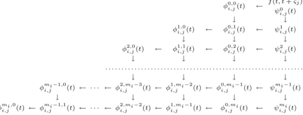
Before proceeding with the proof that the HJM model under [A1]–[A2] can be transformed to a finite dimensional Markovian system, the central idea is illustrated with a diagram. A directed edge, v(t) → w(t), in Figure 2.1 indicates that w(t) occurs in the expression for dv(t). The edges are obtained from Lemma 2.1.
φ0,0i,j(t) ← f(t, t+ςj) ψ0 i,j(t) ↓ ↓ φ1,0i,j(t) ← φ0,1i,j(t) ← ψ1 i,j(t) ↓ ↓ ↓
φ2,0i,j(t) ← φ1,1i,j(t) ← φ0,2i,j(t) ← ψ2i,j(t)
↓ ↓ ↓ ↓
. . . .
↓ ↓ ↓ ↓
φi,jmi−1,0(t) ← · · · ← φ2i,j,mi−3(t) ← φi,j1,mi−2(t)← φ0i,j,mi−1(t)← ψmi−1i,j (t)
↓ ↓ ↓ ↓ ↓
φmi,i,j0(t) ← φi,jmi−1,1(t) ← · · · ← φ2i,j,mi−2(t) ← φi,j1,mi−1(t)← φi,j0,mi(t) ← ψmii,j(t)
Figure 2.1. Interdependence of State Variables.
If [A2] is assumed, then the variables in the lowest level can be expressed as linear combinations of the variables in higher levels, and the diagram can be terminated at depthmi−1. This observation essentially establishes that the HJM model can be transformed to a finite dimensional Markovian system, and is formalised in the following.
Proposition 2.2. Letσi(t, T)satisfy the assumptions [A1] and [A2]. (i) The variablesψmi
i,j(t)andφ γ,mi−γ
i,j (t), for0≤γ≤mi, can be written as linear combinations ofψλ
i,j(t)andφ µ,ν
i,j(t), withλ < mi andµ+ν < mi, in the form
ψmi i,j(t) = mi−1 X λ=0 κi,λ(t+ςj)ψi,jλ (t), φmi,0 i,j (t) = X 0≤µ<ν≤mi−1 κµ,νi (t+ςj)φµ,νi,j−µ(t) + X 0≤ν≤µ≤mi−1 κµ,νi (t+ςj)φ ν,µ−ν i,j (t), φγ,mi−γ i,j (t) = γ X µ=0 κi,µ(t+ςj)φµ,γi,j−µ(t) + mi−1 X µ=γ+1 κi,µ(t+ςj)φγ,µi,j−γ(t),
whereκµ,νi (t+ςj) =κi,µ(t+ςj)κi,ν(t+ςj). (ii) For each1≤j≤m, the variableψ0
n,j(t)can be written as a linear combination of f(t, t+ςj),f(0, t+ςj), andψλ,j0 (t), with 1≤λ≤mi, in the form
ψn,j0 (t) =f(t, t+ςj)−f(0, t+ςj)− n−1
X
λ=1
Proof. (i) The result forψmi
i,j(t) is first established. ψmi i,j(t) = Z t 0 ∂miσ i(s, t+ςj) ∂tmi Z t+ςj s σi(s, u)du ds + Z t 0 ∂miσi(s, t+ςj) ∂tmi dWf i s = Z t 0 "mi−1 X λ=0 κi,λ(t+ςj)∂ λσi(s, t+ςj) ∂tλ # Z t+ςj s σi(s, u)du ds + Z t 0 mi−1 X λ=0 κi,λ(t+ςj) ∂λσ i(s, t+ςj) ∂tλ dfW i s, by [A2] = mi−1 X λ=0 κi,λ(t+ςj) Z t 0 ∂λσi(s, t+ςj) ∂tλ Z t+ςj s σi(s, u)du ds + Z t 0 ∂λσ i(s, t+ςj) ∂tλ dWf i s = mi−1 X λ=0 κi,λ(t+ςj)ψi,jλ (t).
Similar arguments establish the results forφγ,mi−γ
i,j (t).
(ii) For ψ0
n,j(t), recall from (1.8) that f(t, t+ςj) =f(0, t+ςj) +P n λ=1ψ 0 λ,j(t), whence ψn,j0 (t) =f(t, t+ςj)−f(0, t+ςj)− n−1 X λ=1 ψλ,j0 (t).
This establishes the required identities. The main result is now stated.
Theorem 2.3. Letσi(t, T)satisfy the assumptions [A1] and [A2]. Then the HJM model transforms to a Markovian system with state variablesf(t, t+ςj),φλi,µi
i,j (t), andψνi
i,j(t), where the indices i,j,λi,µi, andνi satisfy the restrictions (i) 1≤i≤n,1≤j≤m,0≤λi,0≤µi, and0≤νi< mi,
(ii) for eachi,λi+µi< mi, and(i, νi)6= (n,0). In particular, the system has dimension at mostmPn
γ=1 1 2m
2
γ(mγ+ 3).
Proof. The finite dimensionality and the form of the state variables follow immedi-ately from Proposition 2.2. For the dimension
#{f(t, t+ςj)}=m, #{ψi,jν (t)} ≤m h Pn µ=1mµ −1i, #{φλ,µi,j (t)} ≤mhPn γ=1 1 2mγ(mγ+ 1) i .
Hence the dimension is at mostmPn
γ=1 1 2m
2
γ(mγ+ 3).
The dependence of σi(t, T) on the term structure can be increased by requiring that they satisfy a higher order differential equation, since this allows σi(t, T) to be dependent on forward rates for a larger number of tenors. For smooth volatility functions, the general case in which volatilities depend on the entire term structure can be regarded as a limit of the model introduced in this paper in some sense.
The following result is useful in generating finite dimensional Markovian systems from other finite dimensional Markovian systems.
Proposition 2.4. For each1≤i≤n, fix a positive integerni, and for1≤j≤ni define differential operators
L(j)i = ∂m(j)i ∂Tm(j)i − m(j)i X k=0 κ(j)i,k(T) ∂ k ∂Tk and Li= ni Y j=1 L(j)i . If σi(j)(t, T) satisfiesL(j)i σ (j) i (t, T) = 0, then σi(t, T) =P ni j=1x (j) i (t)σ (j) i (t, T) sat-isfies Liσi(t, T) = 0, wherex(j)i (t)are arbitrary functions of t.
Loosely speaking, Proposition 2.4 implies that finite ‘t-linear’ combinations of
σi(t, T) satisfying [A1]–[A2] again satisfy [A1]–[A2].
3. Examples
This short section lists some volatility functions to which Theorem 2.3 applies. (i) Polynomial Functions. IfLi=
∂k+1
∂Tk+1, then σi(t, T) =
Pk
j=0ci,j(t)Tk.
(ii) Exponential Functions. IfLi= ∂
∂T −λi(T), then σi(t, T) =ci(t)eR0Tλi(x)dx.
In particular, exponential, trigonometric, and hyperbolic functions are spe-cial cases.
(iii) Bessel Functions. IfLi= ∂2 ∂T2 + 1 T ∂ ∂T + 1−m 2 T2 , then σi(t, T) =ci(t)Jm(T),
whereJm(T) is the Bessel function of orderm. (iv) Hypergeometric Functions. If
Li= ∂2 ∂T2 + c −(a+b+ 1)T T(T−1) ∂ ∂T − ab T(T−1),
thenσi(t, T) =ci(t)F(a, b, c;T), where F(a, b, c;T) is the hypergeometric function.
Additional σi(t, T) satisfying the hypotheses of Theorem 2.3 may be obtained by using Proposition 2.4.
4. Generalisation of the Inui-Kijima Model
This section considers a subclass of Markovian systems introduced in§2 that are natural extensions of the [IK98] model. These are the higher order analogues of [IK98] in which the σi(t, T) satisfy the differential equation Liσi(t, T) = 0, where
Li =Qmj=1i [∂/∂T−λi,j(T)]. For certain special cases, explicit expressions for the
bond price are obtained in terms of the state variables, and in particular, the [IK98] formula is obtained in Theorem 4.5.
As in the previous section, let mi be positive integers for 1≤i≤n, and let ςj
be given for 1≤j≤m. Throughout this section, assume [A1]–[A2] with Li= mi Y j=1 ∂ ∂T −λi,j(T) , (4.1)
Lemma 4.1. LetLibe defined as in (4.1), and letci,j:R×Ω→Rfor1≤j≤mi. If σi(t, T)are defined by
σi(t, T) = mi X j=1 ci,j(t)e RT 0 λi,j(x)dx, (4.2) then Liσi(t, T) = 0. Proof. LetLji = Q
k6=j[∂/∂T −λi,k(T)], where 1≤k≤mi. Then
Liσi(t, T) = mi X j=1 ci,j(t)Lji[∂T−λi,j(T)]e RT 0 λi,j(x)dx= 0,
since [∂/∂T−λi,j(T)]eR0Tλi,j(x)dx= 0.
Proposition 4.2. Letσi,j(t, T) =P mi
j=1ci,j(t)e RT
0 λi,j(x)dxas in Lemma 4.1. Then
the corresponding HJM model transforms to a finite dimensional Markovian system with state variables as listed in Theorem 2.3.
Proof. This follows from Theorem 2.3 and Lemma 4.1.
Hence the HJM models considered in this section are Markovian. Considered now are two special cases of the present model for which a bond price formula is available either in terms of the state variables in Theorem 2.3, or a slightly larger set. 4.1. Inui-Kijima-Ritchken-Sankarasubramanian Bond Price Formula. In this subsection, assume m= 1,ς1= 0, andmi= 1, for all 1≤i≤n, so that
Li= ∂
∂T −λi(T) and σi(t, T) =ci(t, r(t))e RT
0 λi(x)dx. (4.3) This is the general [IK98] model, and when n= 1 this is the [RS95] model. For this class of models, a formula for P(t, T) can be obtained in terms of the state variables, and the following identity plays a crucial role.
Lemma 4.3. Theσi(t, T)given by (4.3) satisfy the identities σi(s, t+u) =σi(s, t)e
Rt+u
t λi(x)dx, (4.4)
σi(s, t) =σi(s, s)eRstλi(x)dx. (4.5)
Proof. Since the second identity is a consequence of the first, it is sufficient to prove only the latter. Note, firstly, that
σi(s, t) =ci(s, r(s))e Rt 0λi(x)dx=hc i(s, r(s))e Rs 0λi(x)dxie Rt sλi(x)dx = ˜ci(s, r(s))e Rt sλi(x)dx, where ˜ci(s, r(s)) =ci(s, r(s))eR0sλi(x)dx. Hence σi(s, t+u) = ˜ci(s, r(s))eRst+uλi(x)dx= h ˜ ci(s, r(s))eRstλi(x)dx i eRtt+uλi(x)dx =σi(s, t)e Rt+u t λi(x)dx.
The second identity follows from settingt=sandu= 0 in the above identity. The following lemma is contained in [IK98, p37].
Lemma 4.4. Letβi(t, T) =
RT
t e− Ru
t λi(x)dxdu. Then the following identities hold: Z T t e−Rtuλi(x)dx Z u t e−Rtvλi(x)dxdv du=1 2β 2 i(t, T), (4.6) Z T t σi∗(s, u)du=βi(t, T)σi∗(s, t) +1 2β 2 i(t, T)σ 2 i(s, t), (4.7) Z T t
σi(s, u)du=βi(t, T)σi(s, t), (4.8)
where σi∗(s, u) =σi(s, u)Rsuσi(s, v)dv.
Proof. Denoting by χi(t, T) the term on the left hand side of (4.6)
χi(t, T) = Z T t e−Rtuλi(x)dx Z u t e−Rtvλi(x)dxdv du = Z T t d du Z u t e−Rtvλi(x)dxdv Z u t e−Rtvλi(x)dxdv du = Z T t βi(t, u) d duβi(t, u)du= Z T t d 1 2β 2 i(t, u) = 1 2[βi(t, T)−βi(t, t)] = 1 2β 2 i(t, T), sinceβi(t, t) = 0.
Next (4.7) is proved. From (4.4) Z T t σ∗i(s, u)du= Z T t σi(s, u) Z u s σi(s, v)dv du =σi(s, t) Z T t e− Ru t λi(x)dx Z t s σi(s, v)dv+ Z u t σi(s, v)dv du =σi(s, t) Z T t e− Ru t λi(x)dxdu Z t s σi(s, v)dv+σi2(s, t)χi(t, T),
which is (4.7). Similar arguments establish (4.8).
Finally, the [IK98] formula for the bond price can now be obtained in terms of the state variables. Recall from (2.3) and (2.4) the definition of the state variables
φp,qi,j(t) andψri,j(t). In the present case,j= 1 is the only relevant second subscript, and so the simpler notation φp,qi (t) =φp,qi,1(t) andψr
i(t) =ψi,1r (t) is adopted. Note
that ςi,1= 0.
In view of (1.1) and (1.3), the price of a pure discount bond is given by
P(t, T) = P(0, T) P(0, t) exp " − n X i=1 Z T t ψi0(u)du # . (4.9)
The following bond price formula is contained in [RS95, p60] for the one factor case, and [IK98, p431] for the multifactor case.
Theorem 4.5. If σi(t, T) = ci(t)eR0Tλi(x)dx, then the bond price is given by the
formula
P(t, T) = P(0, T)
where βi(t, T) = RT t e− Ru t λi(x)dxdu, for 1≤i≤n, Φ(t, T) =1 2 n X i=1 φ0,0i (t)βi2(t, T), and Ψ(t, T) = n−1 X i=1 ψi0(t) [βi(t, T)−βn(t, T)].
Proof. Equation (4.9) required computation ofRtTψi0(u)du, which can be expressed as Z T t ψ0i(u)du= Z T t ψ0i(u)du= Z T t Z t 0 σ∗i(s, u)ds+ Z t 0 σi(s, u)dfWsi du = Z t 0 Z T t σi∗(s, u)du ds+ Z t 0 Z T t σi(s, u)du dfWsi = Z t 0 βi(t, T)σ∗i(s, t) + 1 2β 2 i(t, T)σ 2 i(s, t) ds + Z t 0
βi(t, T)σi(s, t)Wfsi by (4.7) and (4.8) =βi(t, T)ψi0(t) +1 2β 2 i(t, T)φ 0,0 i (t),
where Fubini Theorem was used in the third equality. It follows that
n X i=1 Z T t ψ0i(u)du= n X i=1 βi(t, T)ψi0(t) + 1 2β 2 i(t, T)φ 0,0 i (t) = Φ(t, T) + n X i=1 [(βi(t, T)−βn(t, T)) +βn(t, T)]ψ0i(t) = Φ(t, T) + Ψ(t, T) +βn(t, T) n X i=1 ψi0(t) = Φ(t, T) + Ψ(t, T) +βn(t, T) [r(t)−f(0, t)] by (2.8).
This completes the proof.
The following corollary shows that the bond price (4.10) extends to the forward rate dependent volatility case.
Corollary 4.6. Let σi(t, T) be given by (2.1), and satisfy (2.2) with m1 = 1 for all i, so that
σi(t, T) =ci(t, f(t, t+ς1), . . . , f(t, t+ςm))e− RT
t λi(u)du. (4.11)
Then the bond price is again given by (4.10).
Proof. The proof of Theorem 4.5 depends only on Lemma 4.3, which is satisfied by
σi(t, T) in (4.11).
4.2. Constant Coefficient Case. In this subsection, assume λi,j(T) = λi,j are constants, and λi,j=λi,k if and only if j=k. Then
Li= mi Y j=1 ∂ ∂T −λi,j , and σi(t, T) = mi X j=1 ci,j(t)eλi,jT. (4.12) When mi = 1, (4.12) is a special case of the [IK98] model, but this assumption is not made here. For notational convenience, it is assumed that ςj = 0 for all 1≤j≤m, but the results extend trivially to the setting in whichςj are arbitrary.
In order to obtain a bond price formula analogous to Theorem 4.5 for this model, additional state variables need to be introduced.
Lemma 4.7. For each1≤i≤n, define additional state variablesξik,l(t), by ξik,l(t) = Z t 0 ∂kσ i(s, t) ∂tk Z t s ∂lσ i(s, u) ∂ul du ds. (4.13) Then the variables r(t), {ψi,1m(t) | 1 ≤ i ≤ n, 0 ≤ m ≤ mi, (i, m) 6= (n,0)},
{φk,li,1(t)| 1 ≤i ≤ n, k ≥ 0, l ≥0, k+l < mi}, and {ξik,l(t) | 0 ≤ k, l ≤mi}, whereψi,1m(t)andφk,li,1(t)are as defined in (2.3) and (2.4), form a finite dimensional Markovian system.
Proof. In view of Theorem 2.3, it suffices to show that the differentialsdξik,l(t) can be expressed in terms of the state variables. But this follows from
dξik,l(t) = Z t 0 ∂kσi(s, t) ∂tk · ∂lσi(s, t) ∂tl + ∂k+1σi(s, t) ∂tk+l Z t s ∂lσi(s, u) ∂ul du ds dt =hφi,1k∧l, k∨l−k∧l(t) +ξik+1,l(t)idt,
where k∧l = min(k, l) and k∨l = max(k, l). If k ≥ mi or l ≥mi, then as in Theorem 2.3ξik,l(t) can be written as linear combinations ofξµ,νi (t) withµ, ν < mi, sinceλi,j are constants.
The additional state variables introduced in Lemma 4.7 will enable us to obtain a bond price formula, analogous to (4.10).
Let Λi,j(t, T) =ci,j(t)eλi,jT. Then for each integerk≥0 ∂kσi(t, T) ∂tk = mi X j=1 λki,jΛi,j(t, T), (4.14)
and the state variables in (2.3) and (2.4) can be rewritten as follows, where the second and third subscripts have been omitted as in the previous subsection.
φk,li (t) = X 1≤p, q≤mi λki,pλk+li,q Z t 0 Λi,p(s, t) Λi,q(s, t)ds, (4.15) ψmi (t) = X 1≤p, q≤mi λmi,p Z t 0 Λi,p(s, t) Z t s Λi,q(s, u)du ds + X 1≤p≤mi λmi,p Z t 0 Λi,p(s, t)dWfsp. (4.16)
Note that by arguments similar to those used in Lemma 4.3, it is possible to obtain Λi,j(s, t+u) = Λi,j(s, t)eλi,j(u−t)and Λi,j(s, t) = Λi,j(s, s)eλi,j(t−s). (4.17)
For each 1≤i≤n, define themi×mi van der Monde matrixMi by
Mi= h Mij,ki= 1 1 1 · · · 1
λi,1 λi,2 λi,3 · · · λi,mi
λ2
i,1 λ2i,2 λ2i,3 · · · λ2i,mi . . . . λmi−1 i,1 λ mi−1 i,2 λ mi−1 i,3 · · · λ mi−1 i,mi . (4.18)
Since λi,j =λi,k if and only if j=k, by assumption,Mi are invertible. Denoting the inverse of Mi byNi= h Nij,ki, and writing ∂T·σi(t, T) = ∂0σi(t, T) ∂T0 , ∂1σi(t, T) ∂T1 , . . . , ∂mi−1 T σi(t, T) ∂Tmi−1 τ , and (4.19) Λi,·(t, T) = [Λi,1(t, T),Λi,2(t, T), . . . ,Λi,mi(t, T)]
τ
, (4.20)
where the superscriptτ represents matrix transposition, the following identities are
immediately obtained from definitions and (4.14):
Mi× Ni=Imi×mi =Ni× Mi, (4.21)
∂t·σi(t, T) =Mi×Λi,·(t, T), (4.22)
Λi,·(t, T) =Ni×∂T·σi(t, T). (4.23)
Using (4.23) Λi,j(t, T) can be expressed as the linear combination
Λi,j(t, T) = mi X k=1 Nij,k∂ k−1σi(t, T) ∂Tk−1 , (4.24)
where Nij,k areconstants. The following lemma plays a role similar to Lemma 4.4 in the mi= 1 case.
Lemma 4.8. LetΛi,j(t, T)be as defined above, and let βij(t, T) = Z T t eλi,j(u−t)du= 1 λi,j h eλi,j(T−t)−1i, and (4.25) γj,ki (t, T) = Z T t eλi,j(u−t) Z u t eλi,k(v−t)dv du (4.26) = 1 λi,k 1 λi,j+λi,k e(λi,j+λi,k)(T−t)−1− 1 λi,j eλi,j(T−t)−1 .
Then the following identities hold:
Z T
t
Λj,ki (s, u)du=γij,k(t, T) Λi,j(s, t) Λi,k(s, t) + Γj,ki (s, t), (4.27)
Z T
t
Λi,j(s, u)du=βi,j(t, T)Λi,j(s, t), (4.28)
where Λj,ki (s, u) = Λi,j(s, u) Ru s Λi,k(s, v)dv, and Γ j,k i (s, t) =βi,j(t, T) Λ j,k i (s, t). Proof. The arguments used in Lemma 4.4 apply here in view of (4.17).
The bond price formula for the constant coefficient case can now be stated.
Theorem 4.9. Letσi(t, T) =P mi
j=1ci,j(t)eλi,jT, whereλi,j are distinct constants, and let Ni=
h
Nij,kibe the inverse ofMi =
h
Mij,ki=λki,j−1. Then the bond price is given by the formula
P(t, T) = P(0, T)
where Φ(t, T) = n X i=1 X j,k,l,m Nij,lNik,mβi,j(t, T)ξil−1,m−1(t), Ψ(t, T) = n X i=1 X j,k,l,m Nij,lNik,mγij,k(t, T)φil∧m−1, l∨m−l∧m(t), Θ(t, T) = n X i=1 X j,k Nij,kβi,j(t, T)hψki−1(t)−ξki−1,0(t)i,
and1≤j, k, l, m≤mi. Here,l∧m= min (l, m)andl∨m= max (l, m). Proof. As in Theorem 4.5, (4.9) dictates thatPn
i=1
RT
t φ 0
i(u)dumust be computed.
Now for each 1≤i≤n
Z T t φ0i(u)du= Z T t Z t 0 σi(s, u) Z t s σi(s, v)dv ds+ Z t 0 σi(s, u)dWfsi du.
Applying Fubini Theorem, the above integral can be written
Z t 0 " Z T t σi(s, u) Z t s σi(s, v)dv du # ds+ Z t 0 " Z T t σi(s, u)du # dfWsi. LetI1
i(t, T) andIi2(t, T) denote the two integrals above. Then
I1 i(t, T) = X j,k Z t 0 " Z T t Λi,j(s, u) Z u s Λi,k(s, v)dv du # ds by (4.14) =X j,k Z t 0 h γij,k(t, T)Λi,j(s, t)Λi,k(s, t) + Γj,ki (s, t) i ds by (4.27) =X j,k γij,k(t, T) Z t 0 Λi,j(s, t)Λi,k(s, t)ds +X j,k βi,j(t, T) Z t 0 Λi,j(s, t) Z t s Λi,k(s, v)dv ds = X j,k,l,m Nij,lNik,mγij,k(t, T) Z t 0 ∂l−1σ i(s, t) ∂tl−1 · ∂m−1σ i(s, t) ∂tm−1 ds + X j,k,l,m Nij,lNik,mβi,j(t, T) Z t 0 ∂l−1σi(s, t) ∂tl−1 Z t s ∂m−1σi(s, v) ∂vm−1 dv ds = X j,k,l,m Nij,lNik,mβi,j(t, T)ξil−1,m−1(t) + X j,k,l,m Nij,lNik,mγij,k(t, T)φil∧m−1, l∨m−l∧m(t),
where the second last equality follows from (4.24). Summing overi,Pn
i=1I 1
i(t, T) =
Φ(t, T) + Ψ(t, T). NextI2
i(t, T) is considered in a similar fashion.
I2 i(t, T) = X j Z t 0 Z T t Λi,j(s, u)du dWfsi by (4.14) =X j βi,j(t, T) Z t 0 Λi,j(s, t)dWfsi by (4.28) =X j,k Nij,kβi,j(t, T) Z t 0 ∂k−1σ i(s, t) ∂tk−1 dWf i s by (4.24) =X j,k Nij,kβi,j(t, T)hψki−1(t)−ξki−1,0(t)i. Summing over i,Pn i=1I 2 i(t, T) = Θ(t, T), and (4.29) follows.
Remark 4.10. Note that all the arguments in this subsection remain valid even when λk,l=xk,l+i yk,l are complex. So takingmk = 2m0k, and{λk,l} consisting
of conjugate pairs, Theorem 4.9 applies to volatility functions
σi(t, T) = m0i
X
j=1
ci,j(t)exi,jTcos (yi,jT) +di,j(t)exi,jTsin (yi,jT),
which corresponds to taking the operator Li= m0i Y j=1 ∂2 ∂T2−2xi,j ∂ ∂T + (x 2 i,j+y 2 i,j) .
In particular, taking xi,j = 0, the results of this subsection apply toσi(t, T) that are Fourier series like in the variable T.
5. Conclusion
This paper has established very general conditions on the forward rate volatil-ity processes under which the Heath-Jarrow-Morton model transforms to a finite dimensional Markovian system. The characterisations described will allow the con-struction of term structure models with volatility processes that depend on a set of fixed tenor forward rates. Given that only a certain number of fixed tenors are actively traded in most markets, such characterisations should suffice for most practical implementations.
It is evident from Theorem 2.3 that the size of finite dimensional Markovian rep-resentations can grow very rapidly, and consequently themiwould need to be fairly low. With regard to actual implementations, it has already been explained how the implementations of [BC97], [Car94], [RS95], and [IK98] can be represented in this framework. Once a finite dimensional Markovian representation is established, de-rivative prices can be obtained either by solving the PDE, obtained through the application of the Feynman-Kac Theorem, or by Monte Carlo simulation. As a gen-eral rule, it is convenient to apply the PDE approach for low dimensional systems, and to use the Monte Carlo methods for higher dimensional characterisations.
The fact that a formula for the bond price can be obtained is of great utility, since one need only solve the PDE or perform Monte Carlo simulations over the life of the derivative security of interest, which generally is of much shorter maturity than the underlying bond or swap.
Finally some numerical implementations of the models presented in this paper are mentioned. Firstly, Chiarella and El-Hassan [CEH99] have considered the [RS95]
type volatility function and solved the PDE for the American bond option problem using the method of lines. In [BCEHZ99], Bhar, Chiarella, El-Hassan and Zheng consider a volatility process dependent on spot rate and one fixed tenor forward rate. They use the alternating direction implicit method to solve the three spatial variable PDE for the European bond option prices, and compare the results with those obtained using Monte Carlo simulation. This is probably the highest dimension that can be handled conveniently by the PDE methods. In [CEHZ99], Chiarella, El-Hassan and Zheng apply the Monte Carlo methods on forward rate volatilities that depend on the spot rate and a small number of fixed tenor forward rates to evaluate American bond options. Finally, in [CK98a] Chiarella and Kwon develop further the framework of this paper to obtain Markovian transformations of Heath-Jarrow-Morton models with stochastic volatility.
References
[BC97] R. Bhar and C. Chiarella,Transformation of Heath-Jarrow-Morton Models to Mar-kovian Systems, European Journal of Finance3(1997), 1–26.
[BCEHZ99] R. Bhar, C. Chiarella, N. El-Hassan, and X. Zheng,Numerical Methods for Heath-Jarrow-Morton Models with Forward Rate Dependent Volatility Functions, Working paper, School of Finance and Economics, University of Techonology Sydney, 1999. [BG99] T. Bj¨ork and A. Gombani,Minimal Realisations of Interest Models, Working paper,
Stockholm School of Economics, 1999.
[Bj¨o96] T. Bj¨ork,Interest Rate Theory, Financial Mathematics: Bressanone 1996, Springer Verlag Lecture Notes in Mathematics1656(1996), 53–122, ed. W. Runggaldier. [BK91] F. Black and P. Karasinksi,Bonds and Option Pricing when Short Rates are
Log-normal, Financial Analysts Journal (1991), 52–59.
[BM94] A. Brace and M. Musiela, A Multifactor Gauss Markov Implementation of Heath, Jarrow, and Morton, Mathematical Finance4(1994), no. 3, 259–283.
[BS99] T. Bj¨ork and L. Svensson,On the Existence of Finite Dimensional Realisations for Nonlinear Forward Rate Models, Working paper, Stockholm School of Economics, 1999.
[Car94] A. Carverhill,When is Spot Rate Markovian?, Mathematical Finance4(1994), no. 4, 305–312.
[CEH99] C. Chiarella and N. El-Hassan,Pricing American Bond Options in the Heath-Jarrow-Morton Framework, Working paper, School of Finance and Economics, University of Techonology Sydney, 1999.
[CEHZ99] C. Chiarella, N. El-Hassan, and X. Zheng,American Options in the Heath-Jarrow-Morton Framework using Monte Carlo Simulation, Working paper, School of Finance and Economics, University of Techonology Sydney, 1999.
[CIR85] J. Cox, J. Ingersoll, and S. Ross, An Intertemporal General Equilibrium Model of Asset Prices, Econometrica53(1985), no. 2, 386–384.
[CK98a] C. Chiarella and O. Kwon,A Class of Heath-Jarrow-Morton Term Structure Models with Stochastic Volatility, Working paper, School of Finance and Economics, Univer-sity of Techonology Sydney, 1998.
[CK98b] C. Chiarella and O. Kwon,Square Root Affine Transformations of the Heath-Jarrow-Morton Term Structure Model and Partial Differential Equations, Working paper, School of Finance and Economics, University of Techonology Sydney, 1998. [HJM92] D. Heath, R. Jarrow, and A. Morton,Bond Princing and the Term Structure of
Interest Rates: A New Methodology for Contingent Claim Valuation, Econometrica
60(1992), no. 1, 77–105.
[HK79] J. Harrison and D. Kreps, Martingales and Arbitrage in the Multiperiod Security Markets, Journal of Economic Theory20(1979), 381–408.
[HP81] J. Harrison and S. Pliska, Martingales and Stochastic Integrals in the Theory of Continuous Trading, Stochastic Processes and Their Applications 11(1981), 215– 260.
[HW90] J. Hull and A. White,Pricing Interest Rate Derivative Securities, Review of Financial Studies3(1990), 573–592.
[IK98] K. Inui and M. Kijima, A Markovian Framework in Multi-Factor Heath-Jarrow-Morton Models, Journal of Financial and Quantitative Analysis 33(1998), no. 3, 423–440.
[MR97] M. Musiela and M. Rutkowski,Martingale Methods in Financial Modelling, first ed., Springer-Verlag, New York, 1997, Applications of Mathematics30.
[RS95] P. Ritchken and L. Sankarasubramanian,Volatility Structures of Forward Rates and the Dynamics of the Term Structure, Mathematical Finance5(1995), no. 1, 55–72. [Vas77] O. Vasicek,An Equilibrium Characterisation of the Term Structure, Journal of