Optimisation of automatic generation control performance in two-area power system with pid controllers using mepso / Lu Li

Full text

(1)FACULTY OF ENGINEERING UNIVERSITY OF MALAYA KUALA LUMPUR. U. ni. ve r. si. ty. of. M. LU LI. al. ay. a. OPTIMISATION OF AUTOMATIC GENERATION CONTROL PERFORMANCE IN TWO-AREA POWER SYSTEM WITH PID CONTROLLERS USING MEPSO. 2018.

(2) of. M. LU LI. al. ay. a. OPTIMISATION OF AUTOMATIC GENERATION CONTROL PERFORMANCE IN TWO-AREA POWER SYSTEM WITH PID CONTROLLERS USING MEPSO. U. ni. ve r. si. ty. RESEARCH REPORT SUBMITTED IN PARTIAL FULFILMENT OF THE REQUIREMENTS FOR THE DEGREE OF MASTER OF POWER SYSTEM ENGINEEERING. FACULTY OF ENGINEERING UNIVERSITY OF MALAYA KUALA LUMPUR. 2018.

(3) UNIVERSITY OF MALAYA ORIGINAL LITERARY WORK DECLARATION. Name of Candidate: LU LI Matric No:. KQI170006. Name of Degree: Master of Engineering (Power System) Title of Project Paper/Research Report/Dissertation/Thesis (“this Work”): Optimisation of Automatic Generation Control Performance in Two-Area Power. ay. a. System with PID Controllers Using MEPSO. Field of Study: Power System. al. I do solemnly and sincerely declare that:. ni. ve r. si. ty. of. M. (1) I am the sole author/writer of this Work; (2) This Work is original; (3) Any use of any work in which copyright exists was done by way of fair dealing and for permitted purposes and any excerpt or extract from, or reference to or reproduction of any copyright work has been disclosed expressly and sufficiently and the title of the Work and its authorship have been acknowledged in this Work; (4) I do not have any actual knowledge nor do I ought reasonably to know that the making of this work constitutes an infringement of any copyright work; (5) I hereby assign all and every rights in the copyright to this Work to the University of Malaya (“UM”), who henceforth shall be owner of the copyright in this Work and that any reproduction or use in any form or by any means whatsoever is prohibited without the written consent of UM having been first had and obtained; (6) I am fully aware that if in the course of making this Work I have infringed any copyright whether intentionally or otherwise, I may be subject to legal action or any other action as may be determined by UM. Date:. U. Candidate’s Signature. Subscribed and solemnly declared before, Witness’s Signature. Date:. Name: Designation:. ii.

(4) ABSTRACT. Automatic Generation Control (AGC) is used for regulating the electrical power supply in two-area power system and changing the system frequency and tie-line load. The performance of AGC has to be tuned properly so that the performance can be optimized. In this project, modified evolutionary particle swarm optimisation (MEPSO). a. -time varying acceleration coefficient (TVAC) is proposed for an AGC of two-area. ay. power system to optimize its performance by tuning parameters of the PID controllers. Comparison of the performance by using the proposed algorithm and other algorithms. al. was made to identify which algorithm is better in controlling the performance of the. M. AGC. The AGC in two-area power system was constructed and simulated by using. of. MATLAB R2017b software. From the simulation results, it was found that with the same number of PID controllers, the performance of AGC optimised by using MEPSO-. ty. TVAC algorithm is better in terms of overshoot and fitness value than using EPSO and. si. PSO algorithms. Also, using MEPSO-TVAC algorithm, the performance of AGC by. ve r. using two PID controllers is better in terms of rise time and settling time than using one PID controller. Therefore, via implementation of optimisation method, the performance. U. ni. of AGC can be improved by varying the parameters of PID controller.. Keywords: Automatic generation control (AGC), modified evolutionary particle. swarm optimisation-time varying acceleration coefficient (MEPSO-TVAC), PID controller.. iii.

(5) ABSTRAK. “Kawalan Penjanaan Automatik” digunakan untuk mengawal selia bekalan kuasa elektrik dalam sistem kuasa dua kawasan dan mengubah kekerapan sistem dan beban talian tali. Prestasi AGC perlu ditala dengan betul supaya prestasi dapat dioptimumkan. Dalam projek ini, “Pengoptimuman Kawanan Zarah Evolusi. a. Diubahsuai-Pekali Pecutan Berbeza Maza” akan dicadangkan untuk AGC sistem kuasa. ay. dua kawasan untuk mengoptimumkan prestasinya dengan menala parameter pengawal. al. PID. Oleh itu, perbandingan prestasi dengan menggunakan algoritma yang dicadangkan dan algoritma lain akan dibuat untuk mengenal pasti algoritma mana yang lebih baik. M. dalam mengawal prestasi AGC. AGC dalam sistem kuasa dua kawasan dibina dan. of. disimulasikan dengan menggunakan perisian MATLAB R2017b. Dari hasil simulasi, didapati bahawa dengan jumlah pengawal PID yang sama, prestasi AGC dengan. ty. menggunakan algoritma MEPSO-TVAC lebih baik dari segi “overshoot” dan nilai. si. kecergasan daripada menggunakan algoritma EPSO dan PSO. Selain itu, di bawah. ve r. algoritma MEPSO-TVAC, prestasi AGC dengan menggunakan dua pengawal PID adalah lebih baik dari segi “rise time” dan “settling time” daripada menggunakan satu. ni. pengawal PID. Oleh itu, melalui pelaksanaan kaedah pengoptimuman, prestasi AGC. U. dapat ditingkatkan dengan mengoptimumkan parameter pengawal PID.. Kata kunci: Kawalan penjanaan automatik, pengoptimuman kawanan zarah evolusi diubahsuai-pekali pecutan berbeza maza, pengawal PID.. iv.

(6) ACKNOWLEDGEMENTS. Firstly, I would like to thank my supervisor, Assoc. Prof. Ir. Dr. Hazlee Azil Illias for his expertise, assistance, guidance and patience throughout the overall process of doing this project. Without his help, this work would not have been possible.. a. Secondly, I would like to thank and extend my sincere gratitude to one of my. ay. friends, Ms. Susu. She is always willing to encourage and support me when I had difficulty in doing this project. Her advice gives me the strength and confidence to. M. al. overcome problems throughout the entire project.. Lastly, I express my very profound gratitude to my parents for providing me. U. ni. ve r. si. ty. of. with unfailing support and continuous encouragement throughout my years of study.. v.

(7) TABLE OF CONTENTS. Abstract ............................................................................................................................iii Abstrak ............................................................................................................................. iv Acknowledgements ........................................................................................................... v Table of Contents ............................................................................................................. vi List of Figures .................................................................................................................. ix. a. List of Tables.................................................................................................................... xi. al. ay. List of Symbols and Abbreviations ................................................................................. xii. CHAPTER 1: INTRODUCTION .................................................................................. 1 Overview.................................................................................................................. 1. 1.2. Problem statement ................................................................................................... 2. 1.3. Objectives ................................................................................................................ 2. 1.4. Project methodology ................................................................................................ 3. 1.5. Thesis outline ........................................................................................................... 3. ve r. si. ty. of. M. 1.1. CHAPTER 2: LITERATURE REVIEW ...................................................................... 4 Overview.................................................................................................................. 4. ni. 2.1. Automatic Generation Control (AGC) .................................................................... 4. U. 2.2 2.3. The models of power system ................................................................................... 5. 2.3.1. Generator model .......................................................................................... 5. 2.3.2. Load Model ................................................................................................... 6. 2.3.3 Prime mover model.................................................................................................. 7 2.3.4 Governor model ....................................................................................................... 8 2.4. AGC in one Area system ....................................................................................... 10. 2.5. AGC in multi-Area (Two-Area) System ............................................................... 11. vi.

(8) 2.6. Tie-Line Bias Control ............................................................................................ 14. 2.7. PID controller ........................................................................................................ 16 2.7.1. Introduction ............................................................................................... 16. 2.7.2. Proportional Control .................................................................................. 17. 2.7.3. Integral control .......................................................................................... 17. 2.7.4. Derivative control ...................................................................................... 18. ay. a. CHAPTER 3: METHODOLOGY ............................................................................... 19 Introduction............................................................................................................ 19. 3.2. Design AGC in two-area power system with PID controllers ............................... 22. 3.3. Particle Swarm Optimisation (PSO) ...................................................................... 23. 3.4. Evolutionary Particle Swarm Optimisation (EPSO).............................................. 25. 3.5. MEPSO-TVAC ...................................................................................................... 27. 3.6. MEPSO, TVAC, PSO and EPSO parameters selection ........................................ 30. ty. of. M. al. 3.1. si. CHAPTER 4: RESULTS AND DISCUSSIONS ........................................................ 31 Introduction............................................................................................................ 31. 4.2. AGC with two PID controllers (without optimisation) ......................................... 32. 4.3. AGC with two PID controllers (with MEPSO-TVAC optimisation) .................... 34. 4.4. Performances of comparing MEPSO-TVAC with EPSO and PSO for 3 cases .... 36. U. ni. ve r. 4.1. 4.5. 4.4.1. Case I: Two PID controllers in both areas ................................................ 36. 4.4.2. Case II: Only one PID controller in Area 1 ............................................... 39. 4.4.3. Case III: Only one PID controller in Area 2 ............................................. 42. Results and Discussions for each case ................................................................... 46. 4.5.1 Comparison among three algorithms under same number of PID controllers ...... 46 4.5.2 Comparison of different number of PID controllers under MEPSO-TVAC ......... 49 4.5.3 Comparison of the proposed method and previous work …................................. 50 vii.

(9) CHAPTER 5: CONCLUSIONS AND RECOMMDATIONS................................... 51 5.1. Conclusion ............................................................................................................. 51. 5.2. Recommendations for Future Work ...................................................................... 51. U. ni. ve r. si. ty. of. M. al. ay. a. REFERENCES .............................................................................................................. 53. viii.

(10) LIST OF FIGURES. Figure 2.13: Figure 3.1: Figure 3.2: Figure 3.3:. U. a. ay. al. ni. ve r. Figure 3.4: Figure 3.5: Figure 3.6: Figure 4.1: Figure 4.2: Figure 4.3: Figure 4.4: Figure 4.5: Figure 4.6: Figure 4.7: Figure 4.8:. M. Figure 2.9: Figure 2.10: Figure 2.11: Figure 2.12:. of. Figure 2.8:. Page No. Generator block diagram 6 The block diagram of generator and load 6 The simplified block diagram of generator and load 7 A steam turbine block diagram 7 The speed governing system block diagram 8 The steady-state speed characteristics of the governor 8 The speed governing system of steam turbine block 9 diagram The block diagram of load frequency control in one-area 10 system AGC in one-area system block diagram 10 The equivalent circuit of a two-area power system 11 AGC in two-area system block diagram 15 AGC in two-area system with two PID controllers block 15 diagram The block diagram of PID controller 16 The project methodology 19 Model of AGC for two-area power system in Matlab 21 Simulink model of AGC for two-area power system with 22 two PID controllers in Matlab The flowchart of PSO algorithm technique 24 The flowchart of EPSO process 26 The flowchart of MEPSO-TVAC 28 The block diagram of AGC with two PID controllers 32 Power deviation for AGC with two PID controllers 32 Frequency deviation for AGC with two PID controllers 33 The block diagram of AGC with two PID controllers 34 Power deviation for AGC with Two PID controllers 34 Frequency deviation for AGC with two PID controllers 35 The fitness curve for AGC with two PID controllers 35 Difference between EPSO and MEPSO-TVAC on power 36 deviation Difference between EPSO and MEPSO-TVAC on 36 frequency deviation Difference between PSO and MEPSO-TVAC on power 37 deviation Difference between PSO and MEPSO-TVAC on frequency 37 deviation The fitness curve for AGC among EPSO, MEPSO-TVAC 38 and PSO. ty. Figure 2.1: Figure 2.2: Figure 2.3: Figure 2.4: Figure 2.5: Figure 2.6: Figure 2.7:. Title. si. Figure No.. Figure 4.9: Figure 4.10: Figure 4.11: Figure 4.12:. ix.

(11) Figure 4.18: Figure 4.19: Figure 4.20: Figure 4.21: Figure 4.22: Figure 4.23:. 39 40 40 41 41 42 43 43 44 44 45. U. ni. ve r. si. ty. Figure 4.24. 39. a. Figure 4.17:. ay. Figure 4.16:. al. Figure 4.15:. M. Figure 4.14:. The block diagram of AGC with only one PID controller in area 1 Difference between EPSO and MEPSO-TVAC on power deviation. Difference between EPSO and MEPSO-TVAC on frequency deviation Difference between PSO and MEPSO-TVAC on power deviation Difference between PSO and MEPSO-TVAC on frequency deviation The fitness for AGC among EPSO, MEPSO-TVAC and PSO in area 1 The block diagram of AGC with only one PID controller in area 2 Difference between EPSO and MEPSO-TVAC on power deviation Difference between EPSO and MEPSO-TVAC on frequency deviation Difference between PSO and MEPSO-TVAC on power deviation Difference between PSO and MEPSO-TVAC on frequency deviation The fitness for AGC among EPSO, MEPSO-TVAC and PSO in area 2. of. Figure 4.13:. x.

(12) LIST OF TABLES. Title Parameters of a two-area power system The parameters in PSO, EPSO and MEPSO-TVAC for a two-area interconnected power system. Table 4.1: Values of kp, ki and kd for area 1 and area 2 Table 4.2: Optimization values of kp, ki and kd with different optimization methods Table 4.3: Optimization values of kp, ki and kd with different optimization methods Table 4.4: Optimization values of kp, ki and kd with different optimization methods Table 4.5: Results without optimization for two-area power system Table 4.6: Case I results for 3 algorithms for 2 PID controllers in both areas Table 4.7: Case II results for 3 algorithms for only 1 PID controller in area 1 Table 4.8: Case III results for 3 algorithms for only 1 PID controller in area 2 Table 4.9: Results for different number of PID controllers under MEPSO-TVAC Table 4.10: Results for the proposed work and previous work. Page No. 20 30 33 38 42 45 46 46 48 48 49 50. U. ni. ve r. si. ty. of. M. al. ay. a. Table No. Table 3.1: Table 3.2:. xi.

(13) LIST OF SYMBOLS AND ABBREVIATIONS. :. Area control error. ∆𝑃𝑉1. :. Real power command signal in Area 1. ∆𝑃𝑉2. :. Real power command signal in Area 2. ∆𝑃𝐿1. :. Non-frequency-sensitive load change in Area 1. ∆𝑃𝐿2. :. Non-frequency-sensitive load change in Area 2. ∆𝑃𝑚1. :. Mechanical power change in Area 1. ∆𝑃𝑚2. :. Mechanical power change in Area 2. ∆𝑃12. :. Tie-line power change between Area 1 and Area 2. ∆𝜔1. :. Frequency deviation change in Area 1. ∆𝜔2. :. Frequency deviation change in Area 2. of. M. al. ay. a. ACE. Reference set power in Area 1. ∆𝑃𝑟𝑒𝑓2 :. Reference set power in Area 2. U. ni. ve r. si. ty. ∆𝑃𝑟𝑒𝑓1 :. xii.

(14) CHAPTER 1: INTRODUCTION. 1.1. Overview. In recent years, modern power systems are becoming more complex with multiarea and various sources of power generation (Barisal, Mishra, & Chitti Babu, 2018). The large electric power system consists of many control areas interconnected, which. a. are related to the tie-line (Garg & Kaur, 2014). Therefore, the frequency and the tie-line. ay. power of control areas can be disturbed from its scheduled value due to the continuous variation in the load (Sahu, Gorripotu, & Panda, 2016). To avoid this undesirable. al. situation for the power systems, automatic generation control (AGC) mechanism is. M. commonly recommended to be used in the system (Venkatachalam, 2013). It is used to balance the generated power and the demand power in each control area, so that the. of. frequency and tie-line power of the system can be maintained at nominal value or. ty. scheduled value (Salman, 2015). Also, a fast speed and accurate controller is necessary. si. to be used in the electric power system. This is due to a mismatch may happen between. ve r. demand and generation. Then, this mismatch results in the deviation in the frequency from its desired value. The worst thing is that system collapse may be caused by the high frequency deviation (Patel, Singh, & Sahoo, 2013). Hence, the proportional-. ni. integral-derivative (PID) controller is normally recommended to use to maintain the. U. desired system frequency.. Regarding to AGC, many investigations have been conducted in the past. The early works on AGC was introduced by Cohn control theory, which is about AGC designs of interconnected systems (Elgerd & Fosha, 1970). In present days, different control strategies such as adaptive, robust and variable structure have been introduced (P. Kumar & Kothari, 2005). These strategies are based on the different techniques i.e. genetic algorithm (GA) (Jadhav, Vadirajacharya, & Toppo, 2013). In this project, 1.

(15) modified evolutionary particle swarm optimisation-time varying acceleration coefficient (MEPSO-TVAC) algorithm method was implemented to optimize the performance of AGC for a two-area interconnected power system by finding suitable parameters of PID controllers. Evolutionary particle swarm optimisation (EPSO) and particle swarm optimisation (PSO) algorithms were compared with MEPSO-TVAC algorithm in terms of the rise time, settling time, overshoot and fitness function.. a. Problem Statement. ay. 1.2. Automatic generation control (AGC) is one of the most important aspect in. al. power system operation and becomes more pronounced recently by increasing the size,. M. structure and complexity of change in the recovery, especially in two-area power system. Normally, for large-scale power systems of interconnected subsystems or multi-. of. area power control, the connection between control areas is done by using a tie-line.. ty. Each region has its own generator or it is responsible for interchange power with. si. neighboring areas. To ensure the quality of supply, AGC is required to maintain the. ve r. system frequency at nominal value. Hence, optimisation of automatic generation control performance in multi-area power system is important. One of the methods for AGC. ni. optimisation is by using optimisation algorithms.. Objectives. U. 1.3. i.. The objectives of this project are: To construct an automatic generation control (AGC) of two-area power system with PID controllers. ii.. To propose optimization of AGC using modified evolutionary particle swarm optimisation (MEPSO)-time varying acceleration coefficient (TVAC). 2.

(16) iii.. To compare the performance of AGC between without using optimisation, with optimisation and with other optimisation techniques (PSO and EPSO).. 1.4. Project Methodology. The project methodology has 3 main procedures. The first procedure is literature review, which includes relevant theoretical study and previous work. The second. a. procedure is MATLAB simulation which includes the circuit construction, the code. Thesis Outline. al. 1.5. ay. writing and system simulation. The last procedure is report writing.. M. The thesis has five chapters. Chapter 1 presents the overall introduction of this. of. project, problem statement, objectives and simple explanation of project methodology.. Chapter 2 shows the relevant study on the PID controller, automatic generation. ty. control (AGC) and all models in the power system. AGC in a single area system and. ve r. si. AGC in multi-area power system are included.. Chapter 3 describes the overall process of project methodology. Parameters. selection of PSO, EPSO, MEPSO-TVAC algorithm method is set. The circuit diagram. U. ni. in MATLAB of this project is performed.. Chapter 4 explains the simulation results of a two-area power system for. different cases. Also, it shows some discussions in terms of the simulation results.. Chapter 5 summarises the main findings of this project and recommends some possible work for the future.. 3.

(17) CHAPTER 2: LITERATURE REVIEW 2.1. Overview. The literature review includes relevant information about components of main models in the power system and structure of the PID controllers. AGC block diagram in one area system was studied, which is the basic component for constructing the block. Automatic Generation Control (AGC). ay. 2.2. a. diagram of AGC in two-area power system or multi-area power system.. al. Automatic generation control (AGC) system plays an essential role in. M. maintaining system frequency and tie-line power at the nominal value in the large scale multi-area interconnected power system (Sharma, 2016). It means that the balance. of. between the total generations and load losses of the system is required all the time when there is a continuous change in the load (Farshi, Shenava, & Sadeghzadeh, 2015). This. ty. balance is judged by frequent measurements on the system frequency. The system will. si. generate more power than being used when the system frequency is increasing, which. ve r. can accelerate the speed of all the machines. However, when the system frequency is reducing, more load is on the system, making all generators to slow down the speed. U. ni. (Ramakrishna & Sharma, 2010).. In a power system, prime mover drives the electrical generator to convert the. mechanical power to electrical power. Hence, there are three major features of AGC in the electric power system. The first is to keep system frequency at a specified nominal value (Rao & Duvvuru, 2014). The second is to control power flow between interconnected control areas. The control areas are used for controlling generation and load of an interconnected system. The final one is to maintain the generation of each unit at the most economic level (Chandravanshi & Thakur, 2017).. 4.

(18) 2.3. The Models of Power System. Basically, a power system comprises generator, turbine, load and governors. The characteristics of each model for power system are shown in the following sections.. 2.3.1. Generator Model. In a power system, power generating units converts the mechanical power to the. a. electrical power (Ganthia & Rout, 2016). The source of mechanical power comes from. ay. turbine. There is a difficulty in storing the electricity power in a bulk. Hence, it should. al. be sustained between generated power and load demand.. M. The following swing equation of a synchronous machine is applied to small. of. perturbation: 2𝐻 𝑑2 ∆𝛿. = ∆𝑃𝑚 − ∆𝑃𝑒. (2.1). ty. 𝜔𝑠 𝑑𝑡 2. 𝜔𝑠 = mechanical angular velocity. si. where, 𝐻 = equivalent inertia. ve r. ∆𝑃𝑚 = mechanical power change. U. ni. ∆𝑃𝑒 = electrical power change Using small deviation in speed:. 𝑑∆. 𝜔 𝜔𝑠. 𝑑𝑡. 1. = 2𝐻 (∆𝑃𝑚 − ∆𝑃𝑒 ). (2.2). The Laplace Transform function of (2.2) is obtained by: 1. ∆Ω(s) = 2𝐻 [∆𝑃𝑚 (𝑠) − ∆𝑃𝑒 (𝑠)] 𝑠. (2.3). 5.

(19) Hence, according to eq. (2.3), the block diagram of generator is shown in Figure 2.1.. Figure 2.1: Generator block diagram (Saadat,1999). Load Model. a. 2.3.2. ay. In a power system, the load comprises diverse of electrical devices. The. al. electrical power is independent of frequency due to resistive loads such as lighting loads. M. and heating loads. However, motor loads are sensitive to changes in frequency. Hence, the composite of all the driven devices’ speed-load characteristics will determine the. of. sensitivity to frequency (Saadat, 1999).. ty. The speed-load characteristic of composite load is presented by:. (2.4). ve r. si. ∆𝑃𝑒 = ∆𝑃𝐿 + 𝐷∆𝜔. where, ∆𝑃𝐿 = non-frequency-sensitive load change. U. ni. 𝐷∆𝜔 = frequency-sensitive load change. 𝐷 = percent change in load divided by percent change in frequency. Figures 2.2 and 2.3 show the block diagram of generator and load.. Figure 2.2: The block diagram of generator and load (Saadat, 1999) 6.

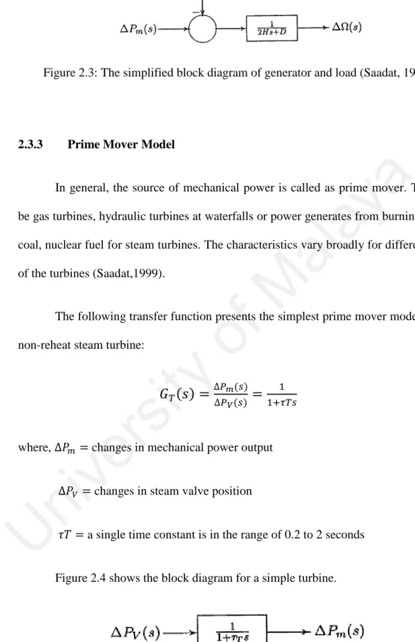
(20) Figure 2.3: The simplified block diagram of generator and load (Saadat, 1999). Prime Mover Model. a. 2.3.3. ay. In general, the source of mechanical power is called as prime mover. They can be gas turbines, hydraulic turbines at waterfalls or power generates from burning of gas,. al. coal, nuclear fuel for steam turbines. The characteristics vary broadly for different types. M. of the turbines (Saadat,1999).. of. The following transfer function presents the simplest prime mover model for the. ty. non-reheat steam turbine:. ∆𝑃𝑚 (𝑠) ∆𝑃𝑉 (𝑠). =. 1 1+𝜏𝑇𝑠. (2.5). ve r. si. 𝐺𝑇 (𝑠) =. where, ∆𝑃𝑚 = changes in mechanical power output. U. ni. ∆𝑃𝑉 = changes in steam valve position 𝜏𝑇 = a single time constant is in the range of 0.2 to 2 seconds. Figure 2.4 shows the block diagram for a simple turbine.. Figure 2.4: A steam turbine block diagram (Saadat, 1999). 7.

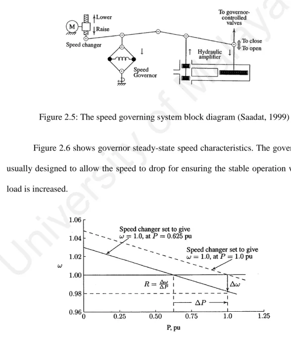
(21) 2.3.4. Governor Model. The governor is the essential component of the power system. It can help to alter the mechanical power output to bring the speed back to a new steady-state level by adjusting the turbine valve when governor detects the changes in speed. Figure 2.5. of. M. al. ay. a. expresses the block diagram of main elements of the speed governing system.. Figure 2.5: The speed governing system block diagram (Saadat, 1999). ty. Figure 2.6 shows governor steady-state speed characteristics. The governors are. si. usually designed to allow the speed to drop for ensuring the stable operation when the. U. ni. ve r. load is increased.. Figure 2.6: The steady-state speed characteristics of the governor (Saadat, 1999). 8.

(22) It can be seen from Figure 2.6 that the slope of curve stands for the speed regulation R. Generally, speed regulation of governors is 5%-6% from 0 to full load. The difference between ∆𝑃𝑟𝑒𝑓 (reference set power) and. 1 𝑅. ∆𝜔 (the power) is ∆𝑃𝑔. (output), which is from speed governor that acts as a comparator (Saadat,1999). 1. The relationship between ∆𝑃𝑟𝑒𝑓 and 𝑅 ∆𝜔 is presented by:. (2.6). ay. 𝑅. a. 1. ∆𝑃𝑔 = ∆𝑃𝑟𝑒𝑓 − ∆𝜔. al. he relation is presented in s-domain is:. 1. M. ∆𝑃𝑔 (𝑠) = ∆𝑃𝑟𝑒𝑓 (𝑠) − ∆Ω(𝑠) 𝑅. (2.7). of. The output ∆𝑃𝑔 is converted to steam valve position command ∆𝑃𝑉 by the. ty. hydraulic amplifier. The simple time constant 𝜏𝑔 is considered. Hence, updated relation. ve r. si. of s-domain is shown as:. ∆𝑃𝑉 (𝑠) =. 1 1+𝜏𝑔. ∆𝑃𝑔 (𝑠). (2.8). ni. Depending on the updated s-domain relation as in eq. (2.8), the speed governing. U. system of steam turbine can be shown as Figure 2.7.. Figure 2.7: The speed governing system of steam turbine block diagram (Saadat, 1999). 9.

(23) 2.4. AGC in One Area System. Based on the descriptions for each model of power system, the block diagram of load frequency control in one-area system is shown as Figure 2.8 by combining all models together. The frequency deviation ∆Ω(s) and the −∆𝑃𝐿 (𝑠) act as the output and. M. al. ay. a. input respectively.. Figure 2.8: The block diagram of load frequency control in one-area system (Saadat,. of. 1999). ty. From the primary load frequency control loop in Figure 2.8, according to speed. si. regulation of governor, a steady-state frequency deviation will be caused by a change in. ve r. the system load. Hence, a reset action can be implemented by the process that an integral controller acts on the load reference setting to change the setpoint of the speed. Then, a reset action is used for reducing the frequency deviation to 0. In order to obtain. ni. a stationary transient response, 𝐾𝐼 integral controller gain is necessary to be adjusted.. U. Figure 2.9 presents block diagram of AGC in one-area power system.. Figure 2.9: AGC in one-area system block diagram (Saadat, 1999) 10.

(24) 2.5. AGC in Multi-Area (Two-Area) System. At the beginning of realizing AGC in the multi-area system, the AGC for a twoarea power system can be studied first. Figure 2.10 shows the equivalent circuit for two. al. ay. a. area power system.. M. Figure 2.10: The equivalent circuit of a two-area power system (Saadat, 1999). of. The following formula states the real power transferred via tie-line when system is at normal operation:. |𝐸1 ||𝐸2 | 𝑋12. sin 𝛿12. (2.9). si. ty. 𝑃12 =. 𝑋𝑡𝑖𝑒 = tie-line reactance. ve r. where, 𝑋12 = 𝑋1 + 𝑋𝑡𝑖𝑒 + 𝑋2 𝛿12 = 𝛿1 − 𝛿2. ni. (2.10). U. Equation (2.9) is used to linearize for a small deviation in ∆𝑃12 (tie-line flow),. the updated model is shown as Equation (2.11): 𝑑𝑃. ∆𝑃12 = 𝑑𝛿12 |𝛿120 ∆𝛿12 = 𝑃𝑠 ∆𝛿12 12. (2.11). where, 𝑃𝑠 = The slope of power angle curve 𝛿120 = 𝛿10 − 𝛿20. 𝛿120 =The initial operating angle. 11.

(25) Then, the updated equation is 𝑑𝑃. 𝑃𝑠 = 𝑑𝛿12 |𝛿120 =. |𝐸1 ||𝐸2 |. 12. 𝑋12. cos ∆𝛿120. (2.12). The equation for tie-line power deviation is defined as: ∆𝑃12 = 𝑃𝑠 (∆𝛿1 − ∆𝛿2 ). (2.13). a. It can be seen from equation (2.13) that the phase angle can determine the. ay. direction of the flow. For example, when ∆𝛿1 > ∆𝛿2, it means that the power will flow. al. from area 1 to area 2, and vice versa. Now, considering ∆𝑃𝐿1 load change in area one, the steady-state frequency deviation for two areas will be the same when the system is. ∆𝜔 = ∆𝜔1 = ∆𝜔2. (2.14). ∆𝑃𝑚1 − ∆𝑃12 − ∆𝑃𝐿1 = ∆𝜔𝐷1. (2.15). si. ty. of. M. in a steady-state status. i.e.,. (2.16). ve r. ∆𝑃𝑚2 + ∆𝑃12 = ∆𝜔𝐷2. The characteristics of governor speed can determine the change in mechanical. U. ni. power by. ∆𝑃𝑚1 =. ∆𝑃𝑚2 =. −∆𝜔 𝑅1. −∆𝜔 𝑅2. (2.17). (2.18). Solving equations (2.15) and (2.17) due to common parameter ∆𝑃𝑚1 , ∆𝜔 will be:. 12.

(26) ∆𝜔 =. −∆𝑃𝐿1 1 1 (𝑅 + 𝐷1 ) + (𝑅 + 𝐷2 ) 1. =. 2. −∆𝑃𝐿1. (2.19). 𝐵1 +𝐵2. 𝐵1 and 𝐵2 are frequency bias factors, given by 1. 𝐵1 = 𝑅 + 𝐷1. (2.20). 1. 𝐵2 = 𝑅 + 𝐷2. (2.21). al. 2. ay. a. 1. M. The following mathematical model stands for the change in the tie-line power: 1 +𝐷2 )∆𝑃𝐿1 𝑅2 1 1 ( +𝐷1 )( +𝐷2 ) 𝑅1 𝑅2. (. (2.22). of. ∆𝑃12 = −. 𝐵2. ty. =𝐵. (−∆𝑃𝐿1 ). si. 1 +𝐵2. ∆𝜔𝑠𝑠 =. −∆𝑃𝐿1 1 1 ( +𝐷1 )+( +𝐷2 ) 𝑅1 𝑅2. (2.23). ni. ve r. The steady-state frequency deviation in per unit is shown by:. U. Therefore, the steady-state frequency deviation states is: ∆𝑓 = (∆𝜔𝑠𝑠 )(𝑓). (2.24). The updated frequency can be expressed as: 𝑓 = ∆𝑓 + 𝑓0. (2.25). 13.

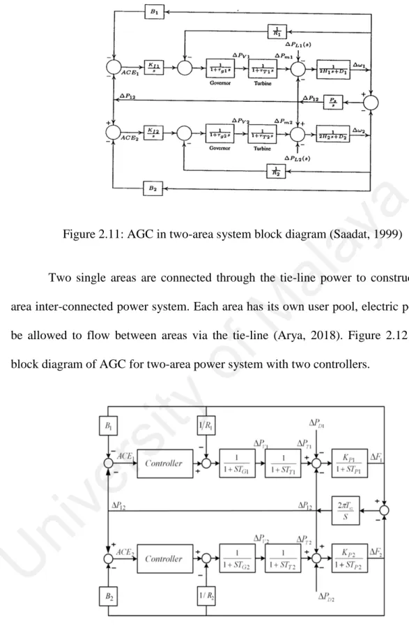
(27) The advantages of multi-area power system are (Sharmili & Livingston, 2015):. Reliable. •. Continuity of supply. •. The Cost/KW for larger generators is less. •. Optimisation of generation. Tie-Line Bias Control. ay. 2.6. a. •. al. For each area, the control error comprises the tie-line error and a linear. M. frequency combination. The mathematical model is shown by equation (2.26),. (2.26). of. 𝐴𝐶𝐸𝑖 = ∑𝑛𝑗=1 ∆𝑃𝑖𝑗 + 𝐾𝑖 ∆𝜔. ACE is called as area control error. The amount of interaction can be determined. ty. by 𝐾𝑖 area bias when a disturbance happens in the neighboring-areas. If 𝐾𝑖 is the same. si. with the frequency bias factor of that neighboring-area, the overall performance can be. U. ni. ve r. acceptable. Hence, the equations of ACEs for two area system are shown: 𝐴𝐶𝐸1 = ∆𝑃12 + 𝐵1 ∆𝜔1. (2.27). 𝐴𝐶𝐸2 = ∆𝑃21 + 𝐵2 ∆𝜔2. (2.28). Figure 2.11 shows a AGC block diagram for two-area power system. In order to avoid the area to enter into a chase mode, it is necessary for the integrator gain constant to maintain at very small level.. 14.

(28) a ay. al. Figure 2.11: AGC in two-area system block diagram (Saadat, 1999). M. Two single areas are connected through the tie-line power to construct a twoarea inter-connected power system. Each area has its own user pool, electric power can. of. be allowed to flow between areas via the tie-line (Arya, 2018). Figure 2.12 shows a. U. ni. ve r. si. ty. block diagram of AGC for two-area power system with two controllers.. Figure 2.12: AGC in two-area system with two PID controllers block diagram (Shakarami, Faraji, Asghari, & Akbari, 2013). 15.

(29) 2.7. PID Controller. 2.7.1. Introduction. The PID controller is called as proportional-integral-derivative controller. It is widely used in process industries as feedback controller (Khodabakhshian & Hooshmand, 2010). The PID controller is robust and can be easily understood. Even though it has varied dynamic characteristics in the process plant, it can still offer. a. excellent control performance (Yusoff & Senawi, 2007). As the name mentions, PID. ay. has the proportional term, the integral term and the derivate term, which are denoted as. al. P, I and D respectively (A. Kumar & Gupta, 2013). The PID controller can improve the. M. transient response through reducing the settling time and overshoot of a system (Daood. ni. ve r. si. ty. of. & Bhardwaj, 2016). Figure 2.13 describes the block diagram of the PID controller.. U. Figure 2.13: The block diagram of PID controller (Ikhe, 2013) 𝑡. 𝑢(𝑡) = 𝐾𝑝 𝑒(𝑡) + 𝐾𝑖 ∫0 𝑒(𝑡)𝑑𝑡 + 𝐾𝑑. where, 𝑢(𝑡) = 𝑐𝑜𝑛𝑡𝑟𝑜𝑙 𝑜𝑢𝑡𝑝𝑢𝑡. 𝑑𝑒(𝑡) 𝑑𝑡. (2.29). 𝑒(𝑡) = 𝑒𝑟𝑟𝑜𝑟 𝑠𝑖𝑔𝑛𝑎𝑙. 𝐾𝑝 = 𝑝𝑟𝑜𝑝𝑜𝑟𝑡𝑖𝑜𝑛𝑎𝑙 𝑔𝑎𝑖𝑛, a tuning parameter 𝐾𝑖 = 𝑖𝑛𝑡𝑒𝑔𝑟𝑎𝑙 𝑔𝑎𝑖𝑛, a tuning parameter. 16.

(30) 𝐾𝑑 = 𝑑𝑒𝑟𝑖𝑣𝑎𝑡𝑖𝑣𝑒 𝑔𝑎𝑖𝑛, a tuning parameter Taking equation (2.29) into Laplace Transfer Function, 𝑈(𝑠) = 𝐾𝑝 𝑒(𝑠) + (𝐾𝑖 ⁄𝑠)𝑒(𝑠) + (𝐾𝑑 𝑠)𝑒(𝑠). 2.7.2. (2.30). Proportional Control. a. P is proportional to the current error value. The proportional gain constant 𝐾𝑝. ay. multiply with the error can adjust the proportional response. Hence, the proportional. al. control part can be given by. (2.31). M. 𝑃𝒐𝒖𝒕 = 𝐾𝑝 𝑒(𝑡). of. The advantage of proportional controller is that it can reduce the rise time but the drawback is that it does not work on eliminating the steady-state error (S. Kumar &. ty. Nath, 2015). The system will be unstable when the proportional gain is very high.. si. However, the control action may make a very weak response to system disturbances. ve r. when the proportional gain becomes too low. The controller can become less sensitive or responsive due to a small gain, which causes a small output response to a large input. ni. error. Hence, based on the tuning theory and a lot of industrial practical, most of the. U. output change should be contributed by the proportional control.. 2.7.3. Integral Control I is proportional to the magnitude and duration of the error respectively. In the. PID controller, the integral is the sum of the instantaneous error over time. It provides the accumulated offset, which has been previously corrected. The integral gain 𝐾𝑖 multiply with the accumulated error. Hence, the integral part is given by. 17.

(31) 𝑡. 𝐼𝒐𝒖𝒕 = 𝐾𝑖 ∫0 𝑒(𝑡)𝑑𝑡. (2.32). The integral part can eliminate the steady-state error and accelerate process movement towards setpoint, but the transient response may become worse due to the response of accumulated errors from the past (S. Kumar & Nath, 2015).. 2.7.4. Derivative Control. ay. a. D is a best estimate of the predicted future values of the control error, which is based on the current rate of change. The magnitude of the derivative term to the entire. 𝑑𝑒(𝑡). M. 𝐷𝒐𝒖𝒕 = 𝐾𝑑. al. control action is defined as the derivative gain 𝐾𝑑 . The derivative part is given by. 𝑑𝑡. (2.33). of. The derivative control is not only beneficial to improve the system stability but. ty. also the transient response. Also, it can reduce the overshoot. Increasing the. si. proportional gain and decreasing the integral gain allowed by the derivative mode will. U. ni. ve r. improve the controller response speed (S. Kumar & Nath, 2015).. 18.

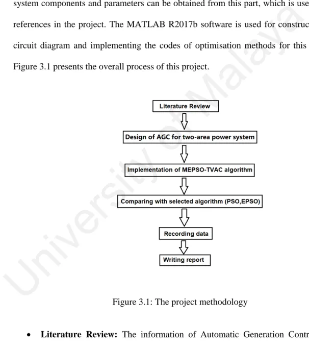
(32) CHAPTER 3: METHODOLOGY. 3.1. Introduction. The project consists of three main parts; literature review, MATLAB software simulation and writing report. The literature review is very helpful in doing a successful research. This is due to most of the relevant information regarding two-area power. a. system components and parameters can be obtained from this part, which is used as the. ay. references in the project. The MATLAB R2017b software is used for constructing the circuit diagram and implementing the codes of optimisation methods for this project.. U. ni. ve r. si. ty. of. M. al. Figure 3.1 presents the overall process of this project.. •. Figure 3.1: The project methodology. Literature Review: The information of Automatic Generation Control, PID controller, MEPSO-TVAC algorithm, EPSO algorithm and PSO algorithm is gathered from the journal papers and books.. 19.

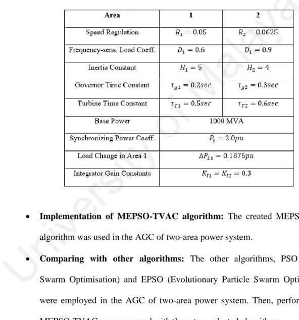
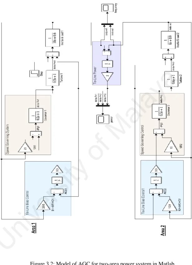
(33) •. Design of AGC for two-area power system: Table 3.1 illustrates parameters of each block for a two-area system connected by a tie-line on a 1000MVA common base (Saadat, 1999). According to parameters from Table 3.1, a basic model of AGC for two-area power system was designed in Matlab Simulink and is shown in Figure 3.2.. ve r. si. ty. of. M. al. ay. a. Table 3.1: Parameters of a two-area power system (Saadat, 1999). •. Implementation of MEPSO-TVAC algorithm: The created MEPSO-TVAC. ni. algorithm was used in the AGC of two-area power system.. U. •. Comparing with other algorithms: The other algorithms, PSO (Particle Swarm Optimisation) and EPSO (Evolutionary Particle Swarm Optimisation) were employed in the AGC of two-area power system. Then, performance of MEPSO-TVAC was compared with these two selected algorithms.. •. Recording data: The obtained results were recorded after implementing the simulation properly.. •. Writing report: The last process is writing report.. 20.

(34) a ay al M of ty si ve r ni U Figure 3.2: Model of AGC for two-area power system in Matlab. 21.

(35) 3.2. Design AGC in two-area power system with PID controllers 1. Based on Figure 3.2, two integrators ( 𝑠 and 0.3) in tie-line control blocks were replaced with two PID controllers respectively. Hence, Figure 3.3 shows the updated. ve r. si. ty. of. M. al. ay. a. AGC model for two-area power system with PID controllers.. Figure 3.3: Simulink model of AGC for two-area power system with two PID. U. ni. controllers in Matlab. 22.

(36) 3.3. Particle Swarm Optimisation (PSO) Particle swarm optimisation is an algorithm optimization method, which was. originally invented by Dr. Kennedy and Dr. Eberhart in 1995 (Xing & Pan, 2018). PSO is used for simulating the social behaviors of animals herding, insects and birds flocking, these swarms are normally searching for food in a collaborative and competition way among the entire population (Seekuka, Rattanawaorahirunkul, & Sansri, 2016).. a. PSO is a population-based optimization tool (Su, Cheng, & Sun, 2011). It can be. ay. used for achieving the optimized objective function. In PSO, each particle has a velocity. al. and a position (Solihin, Lee, & Kean, 2011). Firstly, with certain velocity and position,. M. the particle solutions are initialized randomly. Depending on these positions and velocities, fitness value for each particle is determined. Then, fitness value of each 𝑗. 𝑗. 𝑗+1. and the 𝑋𝑖𝑑. of. particle is used to compare with 𝑝𝑏𝑒𝑠𝑡𝑖𝑑 , which is called the personal best. The 𝑝𝑏𝑒𝑠𝑡𝑖𝑑 named current position of particle will be considered when the fitness. ty. 𝑗. value is better than the 𝑝𝑏𝑒𝑠𝑡𝑖𝑑 . Hence, among the entire particles, the best fitness value. si. 𝑗. ve r. will be set as 𝑔𝑏𝑒𝑠𝑡𝑖𝑑 or the global best value (Illias, Chai, & Abu Bakar, 2016). The updated velocity and position for all particles in the PSO are given by:. ni. 𝑗+1. U. 𝑉𝑖𝑑. 𝑗. 𝑗. 𝑗. 𝑗. 𝑗. = 𝑤𝑉𝑖𝑑 + 𝑐1 𝑟1 (𝑝𝑏𝑒𝑠𝑡𝑖𝑑 − 𝑋𝑖𝑑 ) + 𝑐2 𝑟2 (𝑔𝑏𝑒𝑠𝑡𝑖𝑑 − 𝑋𝑖𝑑 ) 𝑗+1. 𝑋𝑖𝑑. 𝑗. 𝑗+1. = 𝑋𝑖𝑑 + 𝑉𝑖𝑑. (3.1). (3.2). where, 𝑐1 and 𝑐2 = acceleration factors 𝑟1 and 𝑟2 = random constants from 0 to 1 𝑗+1. 𝑉𝑖𝑑 = updated velocity at particle i in dimension d search region. 23.

(37) 𝑗. 𝑉𝑖𝑑 = at iteration j, the velocity of particle i 𝑗. 𝑗+1. 𝑋𝑖𝑑 and 𝑋𝑖𝑑 = current position and updated position respectively of particle i at iteration j in search region of dimension d w = inertia weight. 𝑗𝑚𝑎𝑥. ). (3.3). a. 𝑤𝑚𝑎𝑥 −𝑤𝑚𝑖𝑛. ay. w = 𝑤𝑚𝑎𝑥 − 𝑗(. al. 𝑤𝑚𝑎𝑥 = maximum weight. M. 𝑤𝑚𝑖𝑛 = minimum weight. of. 𝑗𝑚𝑎𝑥 = maximum iteration number. U. ni. ve r. si. ty. The steps of PSO algorithm can be described with flowchart shown in Figure 3.4.. Figure 3.4: The flowchart of PSO algorithm technique (Malik & Dutta, 2014). 24.

(38) 3.4. Evolutionary Particle Swarm Optimisation (EPSO). EPSO optimisation technique was invented by Miranda (Illias & Zhao Liang, 2018). It is a combination of the evolutionary strategies and particle swarm optimisation. Compared with PSO method, EPSO method is more effective and diverse despite starting like PSO. In EPSO, the region of global best fitness value will not be focused by the search of particle. However, the optimum may be found in the. a. neighborhood when the optimal value is not there (Illias, Chai, Abu Bakar, & Mokhlis,. ay. 2015).. 𝑗+1. 𝑉𝑖𝑑. M. al. Hence, the updated velocity is modified from equation (3.1) and is given as 𝑗. 𝑗. 𝑗. 𝑗. ∗ ∗ ∗ ∗ = 𝑤𝑖0 𝑉𝑖𝑑 + 𝑤𝑖1 (𝑝𝑏𝑒𝑠𝑡𝑖𝑑 − 𝑋𝑖𝑑 ) + 𝑤𝑖2 (𝑔𝑏𝑒𝑠𝑡𝑖𝑑 − 𝑋𝑖𝑑 ). (3.4). of. ∗ where, 𝑔𝑏𝑒𝑠𝑡𝑖𝑑 = mutated global best position. 𝑗. (3.5). si. ty. = 𝑔𝑏𝑒𝑠𝑡𝑖𝑑 + 𝜏 ′ 𝑁. ve r. ∗ 𝑤𝑖𝑘 = mutated weight, k = 0, 1 and 2. (3.6). ni. = 𝑤𝑖𝑘 + 𝜏𝑁. U. 𝜏 ′ = noise dispersion factor. 𝜏 = learning dispersion factor. 𝑁 = a random value between 0 and 1. In EPSO, the updated position is obtained using equation (3.2).. 25.

(39) EPSO algorithm uses the concept of replication, mutation and reproduction (Jumaat & Musirin, 2012). Each particle is replicated for replication. For mutation, the weight of each replicated particle is mutated. For reproduction, each particle reproduces an offspring. Then, based on the current position, each particle is evaluated (Illias,. ty. of. M. al. ay. a. Zahari, & Mokhlis, 2016). Figure 3.5 shows the flowchart of EPSO overall process.. U. ni. ve r. si. Figure 3.5: The flowchart of EPSO process (Jumaat & Musirin, 2012). 26.

(40) 3.5. MEPSO-TVAC. The proposed modified evolutionary particle swarm optimization with time varying acceleration coefficient (MEPSO-TVAC) is based on evolutionary particle swarm optimization (EPSO). Based on equation (3.4), a new parameter 𝑟𝑏𝑒𝑠𝑡 is introduced, which is used for providing an extra information to each particle. The advantage of this new term is that it can diversify movement of particles, improve the. ay. premature convergence (Illias, Chai, et al., 2016).. a. exploration capability and behavior of searching for particles. It also can avoid. 𝑗. 𝑗. 𝑗. 𝑗. 𝑗. ∗ ∗ ∗ ∗ ∗ ∗ = 𝑤𝑖0 𝑉𝑖𝑑 + 𝑤𝑖1 − 𝑋𝑖𝑑 ) + 𝑤𝑖3 − 𝑋𝑖𝑑 ) (3.7) (𝑝𝑏𝑒𝑠𝑡𝑖𝑑 − 𝑋𝑖𝑑 ) + 𝑤𝑖2 (𝑔𝑏𝑒𝑠𝑡𝑖𝑑 (𝑟𝑏𝑒𝑠𝑡𝑖𝑑. of. 𝑗+1. 𝑉𝑖𝑑. M. al. The updated velocity for each particle in the MEPSO is given by:. Based on equation (3.6), time-varying acceleration coefficient (TVAC) in the MEPSO. ty. is introduced as follows:. (3.8). ∗ 𝑤𝑖1 = 𝑐1 + 𝜏𝑁. (3.9). ∗ 𝑤𝑖2 = 𝑐2 + 𝜏𝑁. (3.10). ∗ 𝑤𝑖3 = 𝑐3 + 𝜏𝑁. (3.11). U. ni. ve r. si. ∗ 𝑤𝑖0 = 𝑤 + 𝜏𝑁. where, 𝑐1 = cognitive coefficient 𝑐2 = social coefficient 𝑐3 = TVAC for 𝑟𝑏𝑒𝑠𝑡 component ∗ ∗ ∗ 𝑤𝑖1 , 𝑤𝑖2 and 𝑤𝑖3 are all called as mutated weight, where. 27.

(41) 𝑐1 = 𝑐1𝑖 + (𝑐1𝑓 − 𝑐1𝑖 )(𝑗/𝑗𝑚𝑎𝑥 ). (3.12). 𝑐2 = 𝑐2𝑖 + (𝑐2𝑓 − 𝑐2𝑖 )(𝑗/𝑗𝑚𝑎𝑥 ). (3.13). 𝑐3 = 𝑐1 [1 − exp(−𝑐2 𝑗)]. (3.14). where, 𝑐1𝑖 = initial value of cognitive component. ay. M. 𝑐2𝑓 = final value of social component. al. 𝑐1𝑓 = final value of cognitive component. a. 𝑐2𝑖 = initial value of social component. U. ni. ve r. si. ty. which is shown in Figure 3.5.. of. The steps of MEPSO-TVAC algorithm can be described with the flowchart,. Figure 3.6: The flowchart of MEPSO-TVAC (Illias, Chai, et al., 2016). 28.

(42) In MEPSO-TVAC algorithm, cognitive coefficient 𝑐1 is unequal to social coefficient 𝑐2 at each iteration. From equations (3.12) and (3.13), in the initial iteration, when 𝑐1 is large and 𝑐2 is small, it will push the particles to move around the total solution space. With the number of iteration, when 𝑐2 increases but 𝑐1 reduces, each particle’s exploitation and exploration can be improved by the TVAC. The reason for the improvement is that it pulls the particles towards the global solution. However, the. a. particle will be pulled by 𝑐3 towards 𝑟𝑏𝑒𝑠𝑡, it will keep on improving the particle’s. ay. exploration to achieve a better optimum solution. The maximum number of iteration (the stopping criterion) or the cost function is checked to decide whether the steps of. al. 𝑗 𝑗 updating 𝑝𝑏𝑒𝑠𝑡𝑖𝑑 and 𝑔𝑏𝑒𝑠𝑡𝑖𝑑 , updating position and velocity and evaluating the cost. U. ni. ve r. si. ty. of. M. function should be repeated or not (Illias, Chai, et al., 2016).. 29.

(43) 3.6. MEPSO-TVAC, PSO and EPSO parameters selection. At the starting of implementing optimisation methods, some relevant parameters should be declared. The parameters selection is necessary to find the optimized values of 𝐾𝑝 , 𝐾𝑖 and 𝐾𝑑 . For different optimisation methods, the same size of population and number of iteration were used. Table 3.2 presents the values of parameters used in. a. MEPSO-TVAC, EPSO and PSO for two area power system.. ay. Table 3.2: The parameters in PSO, EPSO and MEPSO-TVAC for a two-area. U. ni. ve r. si. ty. of. M. al. interconnected power system. 30.

(44) CHAPTER 4: RESULTS AND DISCUSSIONS. 4.1. Introduction. In order to find the optimum parameters for PID controllers, MEPSO-TVAC optimisation technique was used. PSO and EPSO methods are used for comparing the performance with MEPSO-TVAC method under different cases, which are 2 PID. a. controllers in two areas respectively, 1 PID controller in area 1 and 1 PID controller in. ay. area 2. The only variable that shows a step response is power in area 1 due to a load step in area 1. Hence, the performance can be expressed by settling time, rise time and. al. overshoot of power deviation in area 1. Also, the cost function is defined to determine. M. the best algorithm among the three optimisation methods when the system was run with. of. same number of PID controllers. The definition of each term is as follows:. Settling time: It is the time taken for power system to achieve its steady-state status.. •. Rise time: It is the time taken for the response to increase from 10% to 90% of. ty. •. Overshoot: The overshoot can express how much the peak level is higher than the. ve r. •. si. steady-state response.. steady-state. For example, power system can be damaged when the overshoot is. ni. very high. Hence, the overshoot of power system should maintain as low as. U. possible, which is helpful to protect the power system.. •. Fitness: The fitness is the cost function for the optimisation, which is the error of frequency deviation. It is also the tie-line power. However, this deviation (or error) can be quantified in different ways i.e. overshoot, rise time, settling time. Fitness is a quantity that tells how good the controller is or how good the response of the controller is.. 31.

(45) 4.2. AGC with Two PID Controllers (Without Optimisation). Figure 4.1 presents AGC with two PID controllers for two-area power system block diagram in Matlab Simulink. At the beginning of MEPSO-TVAC algorithm codes, two PID controllers are assumed as the integrator gain constants to reproduce the. si. ty. of. M. al. ay. a. same waveforms as the reference in (Saadat,1999).. U. ni. ve r. Figure 4.1: The block diagram of AGC with two PID controllers. Figure 4.2: Power deviation for AGC with two PID controllers 32.

(46) a ay al. M. Figure 4.3: Frequency deviation for AGC with Two PID controllers. Figure 4.2 and 4.3 show power deviation and frequency deviation for AGC with. of. two PID controllers in two-area power system. ∆𝑃𝑚1 and ∆𝑃𝑚2 represents power. ty. deviation in area 1 and area 2 respectively. ∆𝑃12 stands for tie-line power deviation. si. between area 1 and area 2. Besides, ∆𝜔1 and ∆𝜔2 are frequency deviation in area 1 and. ve r. area 2 respectively. For the following section 4.3 and 4.4, above mentioned parameters represent the same meaning such as ∆𝑃𝑚1 and ∆𝜔1.. ni. Without optimisation, the values of 𝐾𝑝 , 𝐾𝑖 and 𝐾𝑑 for AGC with two PID. U. controllers in area 1 and area 2 are shown in Table 4.1. Table 4.1: Values of 𝐾𝑝 , 𝐾𝑖 and 𝐾𝑑 for area 1 and area 2. 33.

(47) 4.3. AGC with Two PID Controllers (with MEPSO-TVAC Optimisation). Figure 4.4 shows block diagram of AGC with two PID controllers, which is used. ty. of. M. al. ay. a. in MEPSO-TVAC optimization technique.. U. ni. ve r. si. Figure 4.4: The block diagram of AGC with two PID controllers. Figure 4.5: Power deviation for AGC with two PID controllers 34.

(48) a ay. M. al. Figure 4.6: Frequency deviation for AGC with two PID controllers. Figure 4.5 and 4.6 show power deviation and frequency deviation for AGC with. of. two PID controllers in two-area power system using MEPSO-TVAC algorithm respectively. Figure 4.7 shows the fitness for this power system. The fitness value starts. U. ni. ve r. si. ty. from 22.6733 and achieves a steady-state value 16.7952 at the iteration number 56.. Figure 4.7: The fitness curve for AGC with two PID controllers. 35.

(49) 4.4. Performances of comparing MEPSO-TVAC with EPSO and PSO for 3 cases. 4.4.1. Case I: Two PID Controllers in Both Areas. a) EPSO algorithm vs MEPSO-TVAC algorithm. Figure 4.8 and 4.9 present power deviation and frequency deviation using EPSO. si. ty. of. M. al. ay. a. and MEPSO-TVAC algorithm for area 1 and area 2 respectively.. U. ni. ve r. Figure 4.8: Difference between EPSO and MEPSO-TVAC on power deviation. Figure 4.9: Difference between EPSO and MEPSO-TVAC on frequency deviation. 36.

(50) b) PSO algorithm vs MEPSO-TVAC algorithm. Figure 4.10 and 4.11 present power deviation and frequency deviation using. of. M. al. ay. a. PSO and MEPSO-TVAC algorithm on both areas respectively.. U. ni. ve r. si. ty. Figure 4.10: Difference between PSO and MEPSO-TVAC on power deviation. Figure 4.11: Difference between PSO and MEPSO-TVAC on frequency deviation. 37.

(51) c) The fitness among EPSO, MEPSO-TVAC and PSO. Figure 4.12 shows the different fitness for AGC with two PID controllers by using EPSO, MEPSO-TVAC and PSO. It can be clearly seen that fitness value for. si. ty. of. M. al. ay. a. MEPSO-TVAC algorithm is the lowest among three algorithms.. ve r. Figure 4.12: The fitness curves for AGC among EPSO, MEPSO-TVAC and PSO. In the case of two PID controllers on both areas using EPSO, MEPSO-TVAC. U. ni. and PSO, optimization values of 𝐾𝑝 , 𝐾𝑖 and 𝐾𝑑 for each area are shown in Table 4.2. Table 4.2: Optimization values of 𝐾𝑝 , 𝐾𝑖 and 𝐾𝑑 with different optimization methods. 38.

(52) 4.4.2. Case II: Only One PID Controller in Area 1. Figure 4.13 shows block diagram of AGC with only one PID controller in area. of. M. al. ay. a. 1, which is used in EPSO, MEPSO-TVAC and PSO algorithms.. ty. Figure 4.13: The block diagram of AGC with only one PID controller in area 1. U. ni. ve r. si. a) EPSO algorithm vs MEPSO-TVAC algorithm. Figure 4.14: Difference between EPSO and MEPSO-TVAC on power deviation. 39.

(53) a ay. M. al. Figure 4.15: Difference between EPSO and MEPSO-TVAC on frequency deviation. Figure 4.14 and 4.15 show power deviation and frequency deviation using EPSO. of. and MEPSO-TVAC algorithm for area 1 respectively.. U. ni. ve r. si. ty. b) PSO algorithm vs MEPSO-TVAC algorithm. Figure 4.16: Difference between PSO and MEPSO-TVAC on power deviation. 40.

(54) a ay. al. Figure 4.17: Difference between PSO and MEPSO-TVAC on frequency deviation. M. Figure 4.16 and 4.17 show power deviation and frequency deviation using PSO. of. and MEPSO-TVAC algorithm in area 1 respectively.. ty. c) The fitness among EPSO, MEPSO-TVAC and PSO. si. Figure 4.18 shows the different fitness for AGC with only one PID controller in. ve r. area 1 by using EPSO, MEPSO-TVAC and PSO. It can be seen clearly that the fitness. U. ni. value for MEPSO-TVAC algorithm is the lowest despite slower convergence speed.. Figure 4.18: The fitness for AGC among EPSO, MEPSO-TVAC and PSO in area 1 41.

(55) In the case of only one PID controller in area 1 by using EPSO, MEPSO-TVAC and PSO, optimization values of 𝐾𝑝 , 𝐾𝑖 and 𝐾𝑑 in area 1 are shown in Table 4.3.. Case III: Only One PID Controller in Area 2. M. 4.4.3. al. ay. a. Table 4.3: Optimization values of 𝐾𝑝 , 𝐾𝑖 and 𝐾𝑑 with different optimization methods. of. Figure 4.19 shows block diagram of AGC with only one PID controller in area. U. ni. ve r. si. ty. 2, which is used in EPSO, MEPSO-TVAC and PSO algorithms.. Figure 4.19: The block diagram of AGC with only one PID controller in area 2. 42.

(56) a) EPSO algorithm vs MEPSO-TVAC algorithm. Figure 4.20 and 4.21 show power deviation and frequency deviation using EPSO. of. M. al. ay. a. and MEPSO-TVAC algorithm for area 2 respectively.. U. ni. ve r. si. ty. Figure 4.20: Difference between EPSO and MEPSO-TVAC on power deviation. Figure 4.21: Difference between EPSO and MEPSO-TVAC on frequency deviation. 43.

(57) b) PSO algorithm vs MEPSO-TVAC algorithm. Figure 4.22 and 4.23 show power deviation and frequency deviation using PSO. ty. of. M. al. ay. a. and MEPSO-TVAC algorithm for area 2 respectively.. U. ni. ve r. si. Figure 4.22: Difference between PSO and MEPSO-TVAC on power deviation. Figure 4.23: Difference between PSO and MEPSO-TVAC on frequency deviation. 44.

(58) c) The fitness among EPSO, MEPSO-TVAC and PSO. Figure 4.24 shows the different fitness for AGC with only one PID controller in area 2 by using EPSO, MEPSO-TVAC and PSO. It shows that fitness value for. ty. of. M. al. ay. a. MEPSO-TVAC algorithm is the lowest.. si. Figure 4.24: The fitness for AGC among EPSO, MEPSO-TVAC and PSO in area 2. ve r. In the case of only one PID controller in area 2 by using EPSO, MEPSO-TVAC. ni. and PSO, optimization values of 𝐾𝑝 , 𝐾𝑖 and 𝐾𝑑 in area 2 are shown in Table 4.4.. U. Table 4.4: Optimization values of 𝐾𝑝 , 𝐾𝑖 and 𝐾𝑑 with different optimization methods. 45.

(59) 4.5. Results and Discussions for each case. 4.5.1. Comparison among 3 algorithms under same number of PID controller. Based on the simulation results, the important parameters of different cases such as overshoot, fitness and settling time are shown in Tables 4.5 to 4.8. Table 4.5 shows the results without optimisation technique for two-area power system with 2 PID. a. controllers. Table 4.6 presents three algorithms results for 2 PID controllers in both. ay. areas. Table 4.7 shows three algorithms results for only one PID controller in area 1. Table 4.8 presents three algorithms results for only one PID controller in area 2.. al. Without optimisation method, the rise time and settling time are 0.4873s and 14.9948s. M. respectively. The overshoot is 66.6061.. si. ty. of. Table 4.5: Results without optimisation for two-area power system. U. ni. ve r. Table 4.6: Case I results of 3 algorithms for 2 PID controllers in both areas. From Table 4.6, it can be seen that the rise time and settling time for EPSO algorithm are 0.1618s and 2.7672s respectively. The rise time and settling time for MEPSO-TVAC algorithm are 0.2156s and 3.6208s respectively. The rise time and settling time for PSO algorithm are 0.1262s and 4.2374s respectively. Hence, the rise time and settling time for each optimisation algorithm reduced significantly, compared to the results from Table 4.5 (0.4873s and 14.9948s respectively). With optimisation 46.

(60) techniques, the performance of a two-area interconnected power system with 2 PID controllers improves obviously regarding to the rise time and setting time.. When it comes to comparison among 3 different optimisation methods for the same number of PID controllers (one PID controller or two PID controllers), the shortest overshoot and the lowest fitness value is considered in this project compared to rise time and settling time. This is due to there are many parameters and not all are the. a. best for one algorithm. Therefore, using these parameters directly to compare is. ay. undesirable. For example, if the overshoot is higher, then a shorter rise time and settling. al. time can be expected or the other way around. However, a short convergence time is. M. desirable but the lower final cost function value for the optimisation algorithm is preferred. This is also due to the main objective of this project is to achieve the lowest. of. cost function value. Hence, it is important to consider that the best optimisation. ty. algorithm is the one that obtains the lowest overall fitness value.. si. In Table 4.6, the overshoot of MEPSO-TVAC algorithm is 92.7875, which is. ve r. much lower than the other two algorithms. The overshoots of EPSO algorithm and PSO algorithm are 132.7221 and 152.0031 respectively. Then, the final fitness value for MEPSO-TVAC is 16.7952 with the convergence iteration 56, which is much lower than. ni. the other two methods. The final fitness values for EPSO and PSO are 18.6069 with the. U. convergence iteration 95 and 20.3403 with the convergence iteration 66. Hence, for Case I (2 PID controllers on both areas), it is evident that the performance of MEPSOTVAC method is better than EPSO and PSO methods in terms of the lowest overshoot, the lowest fitness value and fastest convergence speed.. In Table 4.7, the overshoot of MEPSO-TVAC algorithm is 83.9833, which is much lower than the other two algorithm methods. The overshoots of EPSO algorithm and PSO algorithm are 107.9056 and 128.9041 respectively. The final fitness value for 47.

(61) MEPSO-TVAC is 16.4276. The final fitness values for EPSO and PSO are 17.4090 with the convergence iteration 66 and 18.1720 with the convergence iteration 17. The most important objective for this project is that achieve the lowest fitness value, which is already mentioned before. Therefore, for Case II (only one PID controller in area 1), it is clearly that performance of MEPSO-TVAC method is better than EPSO and PSO methods in terms of the lowest overshoot and the lowest fitness value.. M. al. ay. a. Table 4.7: Case II results of 3 algorithms for only one PID controller in area 1. of. In Table 4.8, the overshoot of MEPSO-TVAC algorithm is 66.3430, which is. ty. slightly lower than the other two algorithm methods. The overshoots of EPSO algorithm and PSO algorithm are 66.3604 and 66.3619 respectively. The final fitness value for. si. MEPSO-TVAC is 16.5295, which is slighter smaller than the other two algorithm. ve r. methods. The final fitness values for EPSO and PSO are 16.5343 and 16.5352 respectively. Therefore, for Case III (only one PID controller in area 2), the. ni. performance of MEPSO-TVAC method is better than EPSO and PSO methods in terms. U. of the lowest overshoot and the lowest fitness value.. Table 4.8: Case III results of 3 algorithms for only one PID controller in area 2. 48.

(62) 4.5.2. Comparison of different number of PID controllers under MEPSO-TVAC. For comparison of the different number of PID controllers under the same optimisation method, the rise time and settling time can be determined for distinguishing one PID controller or two PID controllers works better in a two-area interconnected power system. This is due to the cost function is different due to different number of PID controllers. For example, less parameters will be considered for. a. one PID controller case than the case of two PID controllers. Hence, using rise time and. ay. settling time for this case is desirable. The main objective for this project is to evaluate. M. MEPSO-TVAC method is used for analysis.. al. the effectiveness of MEPSO-TVAC. Hence, different number of PID controllers under. In Table 4.9, for Case I (2 PID controllers on both areas), the rise time and. of. settling time for MEPSO-TVAC algorithm are 0.2156s and 3.6208s respectively, which. ty. are both much shorter than the other two cases. For Case II (only one PID controller in. si. area 1), the rise time and settling time are 0.2206s and 4.2916s respectively. For Case. ve r. III (only one PID controller in area 2), the rise time and settling time are 0.4936s and 15.2993s respectively. Hence, under MEPSO-TVAC optimisation method, the performance of 2 PID controllers is better than the case of one PID controller in area 1. ni. and the case of one PID controller in area 2 in terms of shortest rise time and shortest. U. settling time.. Table 4.9: Results for different number of PID controllers under MEPSO-TAVC. 49.

(63) 4.5.3. Comparison of the proposed work and previous work. Table 4.10 presents that comparison of the proposed work and previous work. Based on the results from the table, it can be seen that the performance of AGC of twoarea power system for MEPSO-two PID controllers, MEPSO-one PID controller is better than the performance of previous work in terms of the shortest settling time (3.6208s and 4.2916s respectively). Hence, this shows that the proposed work has an. ay. a. obvious improvement than the past developed work.. U. ni. ve r. si. ty. of. M. al. Table 4.10: Results for the proposed work and previous work. 50.

(64) CHAPTER 5: CONCLUSIONS AND RECOMMDATIONS. 5.1. Conclusion. In this project, MEPSO-TVAC algorithm has been successfully implemented on Automatic Generation Control (AGC) with PID controllers for a two-area interconnected power system in MATLAB Simulink software. PSO and EPSO. a. algorithm methods were selected to compare with MEPSO-TVAC algorithm under. ay. different cases.. al. Based on the obtained results, comparison of three cases (Case I: 2 PID. M. controllers on both areas, Case II: one PID controller in area 1, Case III: one PID controller in area 2) shows that the performance for each case of MEPSO-TVAC. of. method is better than EPSO and PSO methods in terms of the overshoot and the final fitness value. Also, with the aid of optimisation methods such as MEPSO-TVAC, the. ty. rise time and settling time for power system are reduced significantly compared to. ve r. si. without optimisation case.. Comparison of different number of PID controllers under MEPSO-TVAC. algorithm shows that the performance for MEPSO-two PID controllers is better than. ni. MEPSO-one PID controller in area 1 and MEPSO-one PID controller in area 2 in terms. U. of the shortest rise time and the shortest settling time.. 5.2. Recommendations for Future Work. Here are some recommendations for future work.. I.. Implement the proposed methods on Automatic Generation Control (AGC) for more than a two-areas in a power system.. 51.

(65) II.. Implement other optimisation methods such as MPSO, MRPSO and GA-PSO. U. ni. ve r. si. ty. of. M. al. ay. a. in the power system with AGC-PID controllers.. 52.

(66) REFERENCES. Arya, Y. (2018). AGC of two-area electric power systems using optimized fuzzy PID with filter plus double integral controller. Journal of the Franklin Institute, 355(11), 4583-4617. doi: 10.1016/j.jfranklin.2018.05.001 Barisal, A. K., Mishra, S., & Chitti Babu, B. (2018). Improved PSO based automatic generation control of multi-source nonlinear power systems interconnected by AC/DC links. Cogent Engineering, 5(1). doi: 10.1080/23311916.2017.1422228. ay. a. Chandravanshi, A., & Thakur, H. S. (2017). Analysis of controllers for automatic generation control of two area interconnected power system. INTERNATIONAL JOURNAL OF ENGINEERING SCIENCES & MANAGEMENT, 7(1), pp433440.. M. al. Daood, E. A., & Bhardwaj, A. K. (2016). Three Area Power System Control System Design using PSO with PID for Load Frequency Control. International Journal of Advanced Research Electrical, Electronics and Instrumentation Engineeering, 5(7), pp.6371-6379. doi: 10.15662/ijareeie.2016.0507090. of. Elgerd, O. I., & Fosha, C. E. (1970). Optimum Megawatt-Frequency Control of Multiarea Electric Energy Systems. IEEE TRANSACTIONS ON POWER APPARTUS AND SYSTEMS, 89(4), pp556-563.. ty. Farshi, H., Shenava, S. J. S., & Sadeghzadeh, A. (2015). Automatic Generation Control of Interconnected HydroThermal System Using Metaheuristic Methods. Majlesi Journal of Energy Management, Vol.4, pp.15-20.. ve r. si. Ganthia, B. P., & Rout, K. (2016). Study of Particle Swarm Optimisation Baesd Interconnected Automatic Generation Control System International Journal of Research in Applied Science & Engineering Technology, 4(VI), pp433-438.. ni. Garg, K., & Kaur, J. (2014). Particle Swarm Optimisation Based Automatic Generation Control of Two Area Interconnected Power System. International Journal of Scientific and Research Publications, 4(1).. U. Ikhe, A. (2013). Load Frequency Control for Interconnected Power System Using Different Controllers. Automation, Control and Intelligent Systems, 1(4), 85. doi: 10.11648/j.acis.20130104.11 Illias, H. A., Chai, X. R., & Abu Bakar, A. H. (2016). Hybrid modified evolutionary particle swarm optimisation-time varying acceleration coefficient-artificial neural network for power transformer fault diagnosis. Measurement, 90, 94-102. doi: 10.1016/j.measurement.2016.04.052 Illias, H. A., Chai, X. R., Abu Bakar, A. H., & Mokhlis, H. (2015). Transformer Incipient Fault Prediction Using Combined Artificial Neural Network and Various Particle Swarm Optimisation Techniques. PLoS One, 10(6), e0129363. doi: 10.1371/journal.pone.0129363. 53.

(67) Illias, H. A., Zahari, A. F. M., & Mokhlis, H. (2016). Optimisation of PID controller for load frequency control in two-area power system using evolutionary particle swarm optimisation. Journal of Electrical Systems, 12(2), pp315-324. Illias, H. A., & Zhao Liang, W. (2018). Identification of transformer fault based on dissolved gas analysis using hybrid support vector machine-modified evolutionary particle swarm optimisation. PLoS One, 13(1), e0191366. doi: 10.1371/journal.pone.0191366. a. Jadhav, A. M., Vadirajacharya, K., & Toppo, E. T. (2013). Application of particle swarm optimisation in load frequency control of interconnected thermal-hydro power systems. International Journal of Swarm Intelligence, 1(1), 91. doi: 10.1504/ijsi.2013.055817. ay. Jumaat, S. A., & Musirin, I. (2012). Evolutionary Particle Swarm Optimisation (EPSO) Based Technique for Multiple SVCs Optimisation. IEEE Iternational Conference on Power and Energy, pp.183-188.. M. al. Khodabakhshian, A., & Hooshmand, R. (2010). A new PID controller design for automatic generation control of hydro power systems. International Journal of Electrical Power & Energy Systems, 32(5), 375-382. doi: 10.1016/j.ijepes.2009.11.006. ty. of. Kumar, A., & Gupta, R. (2013). Compare the results of Tuning of PID controller by using PSO and GA Technique for AVR system. International Journal of Advanced Research in Computer Engineering & Technology, 2(6), pp21302138.. ve r. si. Kumar, P., & Kothari, D. P. (2005). Recent Philosophies of Automatic Generation Ccontrol Strategies in Power System. IEEE TRANSACTIONS ON POWER APPARTUS AND SYSTEMS, 20(1), pp346-357. Kumar, S., & Nath, A. (2015). AUTOMATIC GENERATION CONTROL FOR A TWO AREA POWER SYSTEM USING BACKTRACKING SEARCH ALGORITHM.. U. ni. Malik, S., & Dutta, P. (2014). Parameter Estimation of a PID Controller using Particle Swarm Optimisation Algorithm. International Journal of Advanced Research in Computer and Communication Engineering, 3(3), pp5827-5830. Patel, A. K., Singh, D. K., & Sahoo, B. K. (2013). Automatic generation control of a two unequal area thermal power system with PID controller using Differential Evolution Algorithm. international Journal of Engineering Research and Application, 3(4), pp.2628-2645. Ramakrishna, K. S. S., & Sharma, P. (2010). Automatic generation control of interconnected power system with diverse sources of power generation. International Journal of Engineeering, Science and Technology, 2(5), pp. 51-65. Rao, K. R., & Duvvuru, R. R. (2014). Automatic generation control with nonlinear design of interconnected power system using optimization techniques. INTERNATIONAL JOURNAL OF INNOVATIVE RESEARCH IN ELECTRICAL, 54.

(68) ELECTRONICS, INSTRUMENTATION AND CONTROL ENGINEERING, 2(12), pp2258-2262. Saadat, H. (1999). Power System Analysis. Sahu, R. K., Gorripotu, T. S., & Panda, S. (2016). Automatic generation control of multi-area power systems with diverse energy sources using Teaching Learning Based Optimization algorithm. Engineering Science and Technology, an International Journal, 19(1), 113-134. doi: 10.1016/j.jestch.2015.07.011. a. Salman, G. A. (2015). AUTOMATIC GENERATION CONTROL IN MULTI AREA INTERCONNECTED POWER SYSTEM USING PID CONTROLLER BASED ON GA AND PSO. Diyala Journal of Engineering Sciences, 8(4), pp297-310.. ay. Seekuka, J., Rattanawaorahirunkul, R., & Sansri, S. (2016). AGC Using Particle Swarm Optimisation based PID controller Design for Two Area Power System. IEEE.. M. al. Shakarami, M. R., Faraji, I., Asghari, I., & Akbari, M. (2013). Optimal PID Tuning for Load Frequency Control Using Levy-Flight Firefly Algorithm. 1-5. doi: 10.1109/epecs.2013.6713008. of. Sharma, P. K. (2016). Optimisation of Automatic Generation Control Scheme with Pso Tuned Fuzzy Pid Controller And Comparison with Conventional Pso Pid Controller IOSR Journal of Electrical and Electronics Engineering, 11(1), pp19. doi: 10.9790/1676-11130109. si. ty. Sharmili, A. J., & Livingston, M. A. (2015). Particle Swarm Optimisation based PID controller for two area load Frequency Control System. International Journal of Engineeering Research and General Science, 3(2), pp772-778.. ve r. Solihin, M. I., Lee, F. T., & Kean, M. L. (2011). Tuning of PID Controller Using Particle Swarm Optimisation (PSO). Proceeding of the International Conference on Advanced Science, Engineering and Information Technology 2011, 14(15), pp458-461.. U. ni. Su, T. J., Cheng, J. C., & Sun, Y. D. (2011). Particle Swarm Optimisation with TimeVarying Acceleration Coefficients Based on Cellular Neural Network for Color Image Noise Cancellation. The Sixth International Conference on Digital Telecommunications. Venkatachalam, J. (2013). Automatic generation control of two area interconnected power system using particle swarm optimisation. IOSR Journal of Electrical and Electronics Engineering, 6(1), pp28-36. Xing, H., & Pan, X. (2018). Application of improved particle swarm optimisation in system identification. 1341-1346. Yusoff, W. A. W., & Senawi, A. (2007). Tuning of Optimum PID Controller Parameter Using Particle Swarm Optimisation Algorithm Approach. pp1-7.. 55.

(69)

No results found