Australia
Department of Econometrics and Business Statistics
http://www.buseco.monash.edu.au/depts/ebs/pubs/wpapers/
June 2007
Working Paper 8/07
Estimating the Error Distribution in Multivariate
Heteroscedastic Time Series Models
Estimating the error distribution in multivariate
heteroscedastic time series models
By Gunky Kim, Mervyn J. Silvapulle, and Paramsothy Silvapulle
Department of Econometrics and Business Statistics, Monash University, P.O. Box 197, Caulfield East, Melbourne, Australia 3145.
[email protected], [email protected], [email protected]
Abstract
A semiparametric method is studied for estimating the dependence parameter and the joint distribution of the error term in a class of multivariate time series models when the marginal distributions of the errors are unknown. This method is a natural extension of Genestet al.(1995a) for independent and identically distributed observations. The proposed method first obtains √n-consistent estimates of the parameters of each univariate marginal time-series, and computes the corresponding residuals. These are then used to estimate the joint distribution of the multivariate error terms, which is specified using a copula. Our developments and proofs make use of, and build upon, recent elegant results of Koul and Ling (2006) and Koul (2002) for these models. The rigorous proofs provided here also lay the foundation and collect together the technical arguments that would be useful for other potential extensions of this semiparametric approach. It is shown that the proposed estimator of the dependence parameter of the multivariate error term is asymptotically normal, and a consistent estimator of its large sample variance is also given so that confidence intervals may be constructed. A large scale simulation study was carried out to compare the estimators particularly when the error distributions are unknown, which is almost always the case in practice. In this simulation study, our proposed semiparametric method performed better than the well-known parametric methods. An example on exchange rates is used to illustrate the method.
Some key words: Association; Copula; Estimating Equation; Pseudolikelihood; Semipara-metric. (JEL CLASSIFICATION: C13, C14)
1
Introduction
The multivariate normal distribution continues to play a central role for modeling multivari-ate processes. There are several reasons that justifies such an important role for the normal distribution. For example, often the parameter of interest is a regression coefficient, and its maximum likelihood estimator is usually√n-consistent even if the assumption that the error term is normally distributed is incorrect. In these settings, the error distribution is treated as a nuisance parameter, and valid inferences could be made on the unknown finite dimen-sional parameters. By contrast, there is a range of statistical inference problems where the distribution of the error term is also of interest. In such cases, one does not wish to assume that the error distribution is normal, because the shape of the normal distribution is highly restrictive and hence is likely to be inappropriate for estimating the true error distribution. Estimation of the joint distribution of the error term and learning about the inter-dependence among its components are important topics in statistical inference. This paper provides a rigorous treatment of a method for estimating the joint distribution of the er-ror term in a class of time series models that includes nonlinear Generalized Autoregressive Conditional Heteroscedasticity [GARCH] models.
Let us consider an example to indicate the nature of the topic studied in this paper. The following example is a slightly modified version of that studied by Patton (2006). Let E1,t and E2,t denote the DM-USDollar and Yen-USDollar exchange rates respectively. Let Y1t = logE1,t −logE1,t−1 and Y2t = logE2,t−logE2,t−1. Thus, Y1t and Y2t can be seen as measures of returns of the two investments. We consider the model
Y1t=x1tβ1 +²1t, ²1t= p h1tη1t, h1t=α11+α12²21,t−1+α13h1,t−1, Y2t=x2tβ2 +²2t, ²2t= p h2tη2t, h2t=α21+α22²22,t−1+α23h2,t−1 (1) wherex1tandx2tare some exogenous variables and{(η1t, η2t) :t= 1, . . .}areiid. Thus, after accounting for the effect of the exogenous variables, η1t andη2t represent the undiversifiable risks, in other words, those that are not under the investor’s control. For managing the risks associated with exchange rate fluctuations involving these currencies, the main quantities of interest are functions of the joint distribution of (η1t, η2t). For example, one such quantity is the probability of declines in both exchange rates. More generally, quantities of interest include, pr(Y1t ≤ a1 and Y2t ≤ a2 | xt,Ft−1) and pr(Y1t ≤ a1 | Y2t ≤ a2, xt,Ft−1) where a1 and a2 are given numbers and Ft−1 is the information set up to time (t−1). Clearly
but also the joint distribution of (η1t, η2t).Therefore, this inference problem is different from the standard ones arising in empirical studies involving the GARCH models where one’s main interest involves only the parameter (α, β) in (1).
This type of inference problems, where estimates of the mean and variance functions together with that of the error distribution are required, abound in the financial statistics and risk management literature. In such cases, the typical joint distribution of the error term (η1t, η2t) is skewed and has long tails. Therefore, in the formulation of such inference problems, it is important that the joint distribution of (η1t, η2t) is not assumed to belong to a small parametric family such as the normal. In this area, copulas have been emerging as the natural objects for modeling the joint distribution of (η1t, η2t). First, it would be helpful to recall some elementary facts about copulas.
Let H(x1, . . . , xk) denote the joint cumulative distribution function of a random vector (X1, . . . , Xk) with continuous marginals Fp(xp) = pr(Xp ≤ xp). Then, H has the unique representation H(x1, . . . , xk) = C{F1(x1), . . . , Fk(xk)}, where C(u1, . . . , uk) is the joint cu-mulative distribution of (U1, . . . , Uk) and Up = Fp(Xp) is distributed uniformly on [0,1], p = 1, . . . , k (Sklar (1959)). The function C is called the copula of (X1, . . . , Xk). There has been a substantial interest in the recent literature on copulas for studying multivariate observations. Two of the reasons for such increased interest includes the flexibility it of-fers because it can represent practically any shape for the joint distribution, and its ability to separate the intrinsic measures of association among {X1, . . . , Xk} from their marginal distributions. For an excellent discussion of this see Genest and Favre (2007); for more comprehensive book-length treatments see (Joe (1997), Cherubini et al. (2004), and Nelsen (2006).
It is possible that the distribution functions H, F1, . . . , Fk, and C may belong to para-metric families, for example, H(x1, . . . , xk;α1, . . . , αk, θ) = C{F1(x1;α1), . . . , Fk(xk;αk);θ}. In this case, θ is called the dependence parameter or association parameter. This helps to separate the parameters of the marginal distributions from their intrinsic association, which is nicely captured byθ. An attractive feature of this approach is that the copula C and the association parameter θ are invariant under continuous and monotonically increasing trans-formations of the marginal variables. Hence copulas have an advantage when the interest centers on the intrinsic association among the marginals (Joe (1997), Wang and Ding (2000), Oakes and Wang (2003)).
For the rest of this section, we shall restrict to bivariate copulas for simplicity of nota-tion, but the results would extend in an obvious way to higher dimensions. If the jointcdfof (X1, X2) isC(F1(x1), F2(x2);θ),then the jointpdfof (X1, X2) isc(F1(x1), F2(x2);θ)f1(x1)f2(x2)
where c(·) is the pdf corresponding to C(·). If F1 and F2 are also specified by parametric
families, then the jointpdfwould take the formc(F1(x1;α1), F2(x2;α2);θ)f1(x1;α1)f2(x2;α2),
and maximum likelihood can be applied to estimate (α1, α2, θ). However, the more flexible
Inference Function for Margin [IFM] has emerged as preferable to the method of maximum likelihood. In IFM, the parameters {α1, α2} are estimated in the first stage, and then θ
is estimated in the second stage; see Joe (1997) for an excellent account. If the marginal distributions were known, then, the loglikelihood would take the form
Σn
i=1logc{F1(x1i), F2(x2i);θ}+ Σni=1log{f1(x1i)f2(x2i)}.
Since the marginal distributions are usually unknown, Genest et al. (1995a) developed an elegant theory for estimating θ by the semiparametric method that maximizes the pseudo-likelihood,
Σn
i=1logc{Fˆ1(x1i,Fˆ2(x2i);θ}+ Σni=1log{fˆ1(x1i) ˆf2(x2i}
which is obtained by simply substituting the empirical estimates for the marginal distrib-utions. The possibility of the same method was also indicated in broad terms by Oakes (1994).
Genest et al. (1995a) proved that the asymptotic distribution of the resulting semi-parametric estimator, which we denote by ˜θ, is normal. Kim et al. (2007) reported the results of an extensive simulation study to show that this method is better than its competi-tors. This method was further extended by Kim et al. (2005) to the multivariate regression model, Ypi =x0piβp+εpi,(i= 1, . . . , n, p = 1,2),where the copula of (²1, ²2) was assumed to
have a known parametric form, denoted C(u1, u2;θ). They showed that if ˜βp, a preliminary
√
n-consistent estimator of βp, is available for every p, then the method in Genest et al. (1995a) can be adapted to estimate the copula parameter and hence the joint distribution of (ε1, ε2). In this method, the cdf of εp is estimated by the cdfof the residuals {ε˜p1, . . . ,ε˜pn}, where ˜εpi = Ypi−x0piβ˜p. Now, the semiparametric estimator of the copula parameter θ is argmaxθΣni=1logc{Fˆ1(˜ε1i),Fˆ2(˜ε2i);θ}.
It is clear for these discussions that the essence of the approach in Genest et al.(1995a) and Oakes (1994) is likely to be adaptable in more general settings involving multivariate
regression and time series models whereC(u1, u2;θ) is the copula of the vector of error terms,
provided suitable preliminary estimates of the marginal distributions are available. In this paper, we study one such extension. In particular, our objective of is to provide a complete and rigorous proofs for the extension of the foregoing approach to a class of multivariate time series models and to provide simulation results to show that the proposed method is better than its fully parametric competitors. The proofs are nontrivial, and for this purpose we use recent results of Koul (2002) and Koul and Ling (2006). Their regularity conditions and results play a crucial role in our entire proofs.
Semiparametric estimation of the copula parameter has been studied in detail in Bagdon-avicius et al. (2006) for the case when the marginal variable satisfy a generalized regression model, and essentially the same result of this paper is also used in Chen and Fan (2006) without proofs. Copulas have been used in a very wide range of areas and the literature is quite extensive indeed. The areas include survival analysis, analysis of current status data, censored data and finance (Bandeen-Roche and Liang (2002), Wang (2003), Wang and Ding (2000), Shih and Louis (1995), and Cherubini et al. (2004) ). Joe (1997) and Nelsen (2006) provide comprehensive and authoritative accounts of statistical inference in copulas and de-pendence measures using copulas. Hutchinson and Lai (1990) provides an extensive range of practical examples where copulas are useful.
The plan for the rest of this paper is as follows. In the next section, we state the estimation method more formally. Section 3 presents simulation results to illustrate the superiority of the semiparametric method when the marginal distributions are unknown. Section 4 illustrates the method using a data example. Section 5 concludes. The proofs are given in appendix.
2
Main Results
Let{yi :i= 0,±1,±2, . . .} denote a vector time series, whereyi = (y1i, . . . , yki)0, and let the data generating process be
ypi=µpi(αp1) +εpi and εpi =
q
hpi(αp)ηpi, (2)
where αp = (α0p1, α0p2)0, αp1 ∈ Ωp1, αp2 ∈ Ωp2, Ωp1 and Ωp2 are open subsets in Euclidean
spaces, µpi : Ωp1 → R and hpi : Ωp → R+ are known and twice continuously differentiable functions that may depend on past observations and covariates, and the standardized random
variables{(η1i, . . . , ηki)}are iid. Throughout, we shall assume that the series{ypi}is strictly stationary and ergodic, and that yp0 is independent of all previous observations. Let Ωp = Ωp1×Ωp2, α= (α 0 1, . . . , α 0 k) 0
and α0 denote the true parameter value of α.
LetFpbe the cumulative distribution function of{ηpi}and letfpdenote the corresponding density function. LetC(u;θ) andc(u;θ) denote the copula ofηand the corresponding density function, respectively, where u = (u1, . . . , uk)0 and η = (η1, . . . , ηk)0. Let F = (F1, . . . , Fk),
F(ηi) = (F1(η1i), . . . , Fk(ηki)),and F(η) = (F1(η1), . . . , Fk(ηk)).For simplicity, we shall treat the case when θ is a scalar. The main results for the vector case are stated later.
Let us temporarily suppose thatFp andfp are completely known. Now, the loglikelihood takes the form,
`∗(θ, α) =L∗(θ;α,F) +B(α, f1, . . . , fk) where L∗(θ;α,F) = Plogc{F(η
i);θ} and B(α, f1, . . . , fk) =
P
log{f1(η1i). . . fk(ηki)}. By standard results, the maximum likelihood estimator of (θ, α), which is Argmax `∗(θ, α), is
consistent and asymptotically normal provided the model is correctly specified.
Now, let us relax the temporary assumption and suppose that (F1, . . . , Fk) is unknown, which is usually the case in practice. In this case we modify the foregoing method for estimating θ. Let Fpn(t) = (n + 1)−1Σni=1I(ηpi ≤ t), the rescaled empirical distribution function [edf] of {ηpi : i = 1, . . . , n}. The difference between Fpn and the usual empirical distribution function is that the denominator isn+ 1 instead of n.
We assume that the time series model (2) can be estimated for each margin separately, and let ˜αp denote a
√
n−consistent estimator of α0
p, (p = 1, . . . , k). Now, the residuals corresponding to {ηpi} can be estimated by
˜
ηpi = [ypi−µpi(˜αp1)]/
q
hpi(˜αp). (3)
Let ˜Fpn(t) = (n+ 1)−1Σni=1I(˜ηpi ≤ t) and ˜Fn(ηi) = ( ˜F1n(η1i), . . . ,F˜1n(η1i)); thus, ˜Fpn(t) is the edfof the residuals{η˜pi}. Now, a natural generalization of the approach in Genestet al. (1995a) and Oakes (1994) for iid observations suggests that an estimate ˜θ of θ is given by
˜
θ = argmaxθ L(θ) where L(θ) = Σ logc{F˜n(˜ηi);θ}. (4) Since ˜Fn is expected to be close to F for large n, we would expect L(θ) to be close to the loglikelihood, Σ logc{F(ηi);θ}, except for a constant term and hence one would expect that ˜
We will show that ˜θ is consistent and asymptotically normal, propose a consistent esti-mator of its large sample variance, and evaluate these by simulation studies.
Theorem 1. Suppose that the regularity condition A in the Appendix is satisfied. Letα˜ be a
√
n-consistent estimator ofα and letθ˜denote the estimator ofθ defined in (4). Let `(θ, u) = logc(u1, . . . , uk;θ), `θ(θ, u) = (∂/∂θ)`(θ, u),and`θ,p(θ, u) = (∂2/∂θ∂up)`(θ, u1, . . . , uk).Then, ˜
θ is a consistent estimator of θ0 and the asymptotic distribution of n1/2(˜θ−θ0) is N(0, ν2), where ν2 =σ2/γ2, γ =−E£l θ,θ{θ0,F(η)} ¤ , σ2 =var£lθ{θ0,F(η)}+W1(η1). . .+Wk(ηk) ¤ , and Wp(ηp) = Z I¡Fp(ηp)≤up ¢ lθ,p(θ0, u)dC(u;θ0). (5)
Further, a consistent estimator ν˜2 of ν2 is given by ν˜2 = ˜σ2/γ˜2, where
˜ γ =−n−1Σn i=1lθ,θ{θ,˜ F˜n(˜ηi)}, σ˜2 = Sample variance of {T˜1(˜θ), . . . ,T˜n(˜θ)}, ˜ Ti(θ) =lθ{θ,F˜n(˜ηi)}+n−1Σkp=1Wp(˜ηpi, θ), i= 1, . . . , n, and W˜p(˜ηpi, θ) =n−1Σnj=1I ¡˜ Fpn(˜ηpi)≤F˜pn(˜ηpj) ¢ lθ,p{θ,F˜n(˜ηj)}. (6)
Genest et al. (1995a) showed that the foregoing semiparametric method for iid observa-tions is fully efficient for the independent copula. Since ν2 is the same as that for the iid
setting, it follows that the foregoing result of Genest et al. (1995a) holds for the time series model in (2).
Theorem 1 holds when θ is a vector parameter as well. This is stated below. The proof is essentially the same as that for the case when θ is a scalar.
Theorem 2. Let the setting be as in Theorem 1 except that θ is a vector. Let φ(u;θ) denote (∂/∂θ) log{c(u;θ)}. Then, n1/2(˜θ − θ
0) converges in distribution to N(0, V) where V = B−1ΣB−0, B = R(∂/∂θ0)φ(u;θ
0)dC(u;θ0), and Σ is the covariance matrix of the m-dimensional random vector whose jth component is
φj{F(η);θ0}+ Σkp=1
Z
I{Fp(ηp)≤up)(∂/∂up)φj(u;θ0)dC(u;θ0), j = 1, . . . , m.
An estimator of the covariance matrix V is Vˆ = ˆB−1Σ ˆˆB−0 where Σˆ is the sample covari-ance matrix of {T˜1φ(˜θ), . . . ,T˜φ
n(˜θ)}, T˜iφ(θ) = φ{F˜n(˜ηi);θ} + ˜W1φ(˜η1i, θ) + . . .+ ˜Wkφ(˜ηki, θ), ˜
Wφ
3
Simulation Study
Since the main results on the properties of the proposed semiparametric method are asymp-totic, a large scale simulation study was carried out to compare its properties with other competing ones, namely MLE and IFM.
Design of the study:
The models for the two margins are: y1t = h1tη1t, h1t = 0.2 + 0.1y1,t−1 + 0.15h1,t−1 and y2t=h2tη2t, h2t = 0.1 + 0.1y2,t−1+ 0.15y2,t−1+ 0.1h1,t−1.
The following copulas were considered in the study.
(1) Ali-Mikhail-Haq [AMH] Family of copulas: C(u, v;θ) =uv/{1−θ(1−u)(1−v)}. (2) Frank copula: C(u, v;θ) = −θ−1log¡[1 + (e−θu−1)(e−θv −1)]/(e−θ−1)¢
(3) Gumbel copula: C(u, v;θ) = exp−¡(−logu)θ+ (−logv)θ¢1θ
(4) Joe copula: C(u, v;θ) = 1−¡(1−u)θ+ (1−v)θ−(1−u)θ(1−v)θ¢1θ (5) Plackett copula: C(u, v;θ) = [1 + (θ−1)(u+v)− {{(1 + (θ−1)(u+v)}2−4θ(θ−1)uv}12]/{2(θ−1)}. (6) Gaussian copula: C(u, v;θ) = R−∞Φ−1(u)R−∞Φ−1(v){2π(1−θ2)1/2}−1exp[{2(1−θ2)}−1(2rst−s2−t2)]2dsdt (7) Student-t copula: C(u, v;θ) = Rt−ν1(u) −∞ Rt−1 ν (v) −∞ {2π(1−θ2)1/2}−1[1 +{(s2+t2−2θst)/{ν(1−θ2)}]−(ν+2)/2dsdt Error Distributions: The following pairs of marginal distributions were considered for the error distribution: (1)η1 andη2 are normally distributed, (2)η1 ∼tr andη2 ∼tr,(3)η1 ∼tr and η2 ∼ skewtr with skewness = 0.5, and (4) η1 ∼tr andη2 ∼χ25.The values 3 and 8 were
considered for r in tr.
The IFM and ML methods in this simulation assume that the marginal error distrib-utions are all normal. Therefore, the first pair of error distribdistrib-utions corresponds to the correct specification of the marginal distributions, while each of the other three leads to a misspecification of the model. A skewed-tr distribution has tails that are of the same order as that for tr but the probability masses on either sides of the origin are different, leading to skewness. Since the semiparametric method estimates each marginal distribution nonpara-metrically, it is meant to be used when the sample size is moderate to large. This is not a concern because data sets used for modeling GARCH type models are usually very large. For such models, 100 observations is of course very small. In this study, we considered sample sizes 100 and 500. This captures a broad range of realistic settings. All the computations
were programmed in MATLAB Version 7.0.4 and optimizations were performed using the procedure ”fmincon.m” in the ”Optimization Toolbox (3.0.2).
The values for the copula parameter θ were chosen so that the corresponding Kendall’s tau takes the values 0.2, 0.5 and 0.8, except for the Ali-Mikhail-Haq family because its tau value cannot be as high as 0.5. Therefore, for this copula we chose the τ values -0.1, 0.1 and 0.2. The foregoing seven copulas cover a very wide range of distributional shapes for the errors, and the error distributions also cover a very broad range. Thus, the design of the simulation covers a broad range of realistic settings.
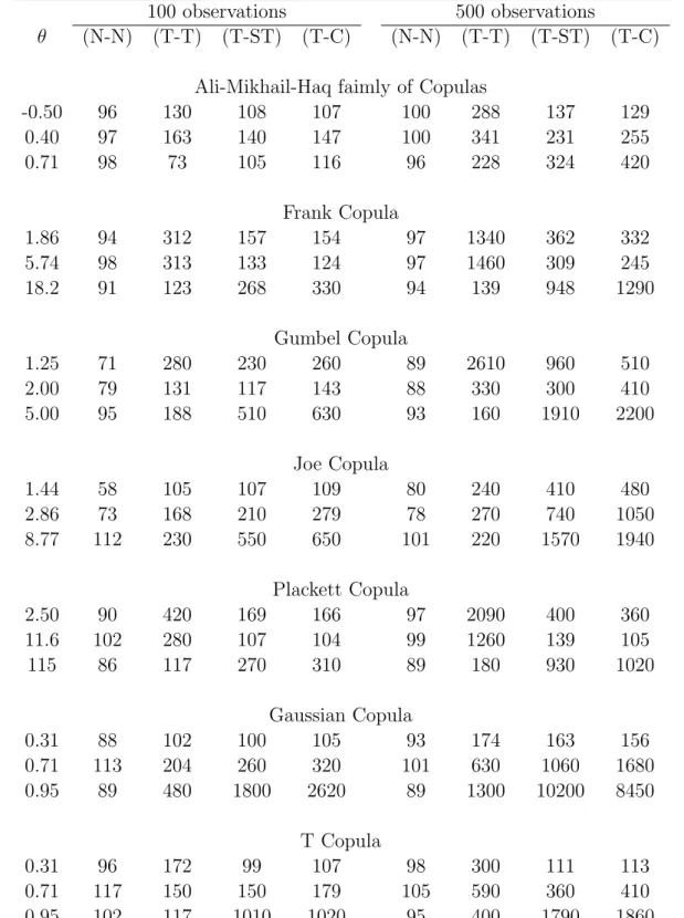
Results:
The differences between the performance of IFM and ML estimators were small, with the IFM performing slightly better. Since IFM is now well accepted in the copula literature, we evaluate the performance of the semiparametric method relative to the IFM method. Each marginal distribution is correctly specified as normal:
The results are given in Table 1 under the heading N-N. Since the marginal distribu-tions and the copula are correctly specified, there is no misspecification for the IFM method. Consequently, as expected, the IFM estimator performs better than the semiparametric esti-mator. However, the differences between these estimators are small. These results show that, even if the error distribution is known, the use of the semiparametric method in Theorem 1, which ignores the fact that the error distribution is known, does not suffer significant loss of efficiency.
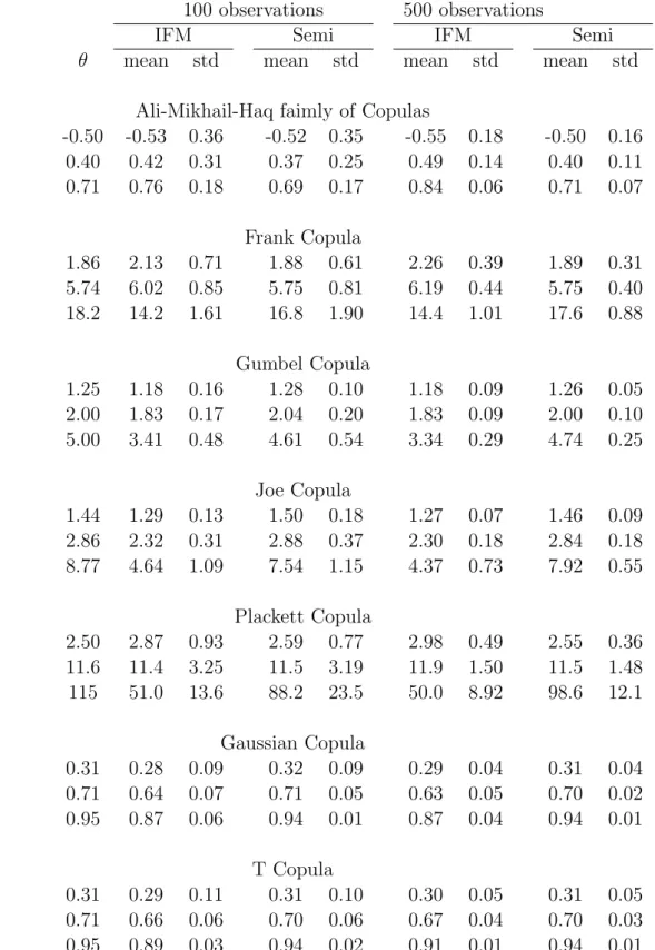
Each marginal distribution is incorrectly specified as Normal:
Table 2 provides means of the simulated estimates of θ when the two marginal error distributions areT3andχ25.The same table also provides standard deviations of the simulated
estimates ofθ.Table 2 shows that if the error distribution is misspecified then the distribution of the IFM estimator may be centered at a value that is quite different from the true value of θ.Tables 1 and 2 show quite clearly that (i) the IFM estimator is highly nonrobust against misspecification of the marginal distributions, and (ii) the distribution of the semiparametric estimator is centered around the true value ofθand is far superior to the IFM estimator ofθ. The very large values for relative MSE in Table 1 reflect the fact that misspecification of the marginal distribution may result in the IFM estimator being inconsistent, and consequently, turns out to be substantially worse than the semiparametric estimator.
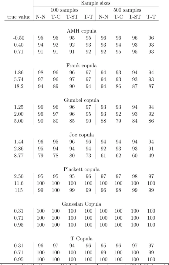
The coverage rates of a large sample 95% confidence interval based on a normal approx-imation for the large sample distribution of ˜θ given in Theorem 1, are provided in Table 3. This table shows that the coverage rates are close to 95% in most cases. The coverage rates tend to drop for some copulas when the parameter is close to the boundary. Overall, these results show that the semiparametric method offers a reliable and easy to compute large sample confidence interval for θ.
In summary, the semiparametric estimator ˜θ is better than the parametric ML and IFM estimators, and Theorem 1 provides the main results for implementing this semiparametric method for statistical inference.
4
An Example
In this section we briefly discuss an example to illustrate the semiparametric method pro-posed in section 2. This is a simpler version of the model developed and studied in detail by Patton (2006), to which we refer the readers for detailed discussions about the practical aspects of the problem. LetY1t and Y2t denote the log difference of DM-USD and Yen-USD exchange rates respectively, as defined in the Introduction. We consider the model
Y1t =µ1+²1t, ²1t = p h1tη1t, h1t=α11+α12²21,t−1 +α13h1,t−1, Y2t =µ2+²2t, ²2t = p h2tη2t, h2t=α21+α22²22,t−1 +α23h2,t−1 (7) We assume that{η1t, η2t}areiid, and letC(u1, u2;θ) denote their copula. The main purpose
of the methodology introduced in the earlier sections was to estimate θ, and to estimate the joint distribution of {η1t, η2t} when its marginal distributions are unknown.
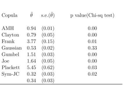
We use the data for the period Jan 1991 - Jan 1999, which is the period prior to the introduction of the Euro. The total number of observations is 2046. Thus, we have a reasonably large number of observations. We estimated several copulas. The estimates and their standard errors are given in Table 4. To assess the goodness of fit of the estimated copulas, we adopted a method similar to that in Patton (2006). We applied a chi-square goodness of fit with the unit square, the support of the copula, divided into 100 cells. To this end, we adopted the method in Junker and May (2005). The cells were formed by grid-lines parallel to the two axes. Each cell with small count was merged with a neighbouring one. The expected count for each cell was estimated by substituting the estimates for the copula parameters. Since such an estimation involves a nonparametric estimator namely the
empirical distribution functions of the marginals, it is not clear that the chi-square statistic would be approximately chi-square distributed. In any case, we computed the p-values corresponding to a chi-square distribution. These are given in Table 4. Since the sample size is large, it is likely that the p-values in Table 4 are reasonably reliable. Despite this caveat, these p-values can be compared among themselves to rank the models in terms of the goodness of fit. The indications are that the Gaussian copula provides the best fit.
For the Gaussian copula, the estimated distribution of (η1t, η2t), conditional on Ft−1 is C( ˜F1n(˜η1),F˜2n(˜η2); 0.53) where ˜F1n and ˜F2n are the empirical distribution functions of the residuals{η1t}and {η2t}respectively, andC(u1, u2;θ) is the Gaussian copula. Based on this
estimated joint distribution, we can write down the estimated joint distribution of (y1t, y2t) conditional on the history up to time t−1. This estimated joint distribution can then be used for estimating various quantities of interest. To illustrate this, we consider the following two quantities: A(c) = P{E1,T ≤ cE1,T−1, E2,T ≤ cE2,T−1 | FT−1} and B(c) = P{E1,T ≤ cE1,T−1 | E2,T ≤ cE2,T−1,FT−1}, where c > 0. Thus, A(1) is the probability that both
exchange rates fall at timeT given the history up to that time, andA(0.9) is the probability that both exchange rates fall to 90% of the value on the previous day, given the history up to that time. Similarly,B(1) is the probability that the first exchange rate falls at timeT given that the second has fallen and the history up to that time. Substituting directly into the estimated distribution of (y1t, y2t), we obtain the estimates 0.333, 0.247, and 0.106 for A(c) forc= 1, 0.9 and 0.7 respectively. Similarly, estimates ofB(c) forc= 1, 0.9 and 0.7 are 0.498, 0.425, and 0.268 respectively. Note that these estimates are obtained without assuming any parametric functional form for the marginal error distributions. Theorem 1 says that this is a valid method. This is in contrast to other more familiar methods that would assume particular parametric forms such as bivariate normal or bivariate t-distributions. Such a method would not be valid if the assumed distribution is incorrect, which is most likely to be the case in practice. This exemplifies the importance of the semiparametric method proposed in this paper.
5
Conclusion
We developed a semiparametric method for estimating the dependence parameter and the joint distribution of the error terms in a class of multivariate nonlinear GARCH models. The method has two stages. In the first stage, parameters of the GARCH model are estimated
separately for each margin. In the second stage, the empirical distribution of the residuals is used as an estimate of the true error distribution for each margin, which in turn is substituted in the likelihood function to estimate the copula parameter. The nonparametric part of the semiparametric method estimates the error distribution of each margin by the empirical of the residuals. Consequently, the method does not require knowledge of the marginal error distributions. This is a very appealing feature of this method.
We showed that the proposed semiparametric estimator is asymptotically normal. It turns out that the form of the asymptotic variance is a natural extension of that obtained by Genest et al.(1995a) for the case when the observations are independent and identically distributed. This helped us to use their results and construct consistent estimates for the as-ymptotic variance and confidence interval for the dependence parameter. Simulation results showed that our semiparametric estimator performs significantly better than the parametric ones when the true error distribution deviates from that assumed by the parametric meth-ods, maximum likelihood and inference function for margins. This is important because the true error distribution is usually unknown in practice. We conclude that the semiparametric method proposed here is better than its main competitors, namely maximum likelihood and inference function for margins, for estimating the joint distribution of the error terms in linear and nonlinear GARCH models.
6
Appendix
As in the text, the indexprefers to thepth component. For notational simplicity, we provide the proof for the bivariate case and hencep= 1 or 2.However, only minor changes to notation are needed for the higher dimensional case. For example, the loglikelihood l(θ, u1, u2) for
the bivariate case would need to be written as l(θ, u1, . . . , uk) for the multivariate case. For simplicity of notation/expression, we shall avoid writing ‘for every p’ or ‘p= 1,2’, as far as possible.
Let H(θ, u1, u2) denote a derivative of l(θ, u1, u2) up to third order in θ and second
or-der in (u1, u2). Let (U1, U2) denote a random vector with the same distribution as that of
(F1(η1), F2(η2)) so that (U1, U2)∼C(u1, u2;θ0).For any functiong(x), let ˙g(x) = (∂/∂x)g(x)
and letkgk= supx|g(x)|.To simplify notation, we shall writeµpi(αp) forµpi(αp1) so thatµpi is treated as a function of the same vector parameterαp which is defined as (α0p1, α0p2)0.Thus,
Let
anp,i = ˙µpi(α0p)/
q
hpi(α0p) and bnp,i = ˙hpi(α0p)/{2hpi(α0p)}. (8) The variables anp,i and bnp,i may be seen as standardized forms or explanatory variables for the mean and the variance functions, respectively, of ypi.
Now, let us introduce the following regularity conditions. Condition A:
(A.1): The distribution function Fp has continuously differentiable density, denoted by fp and it satisfies supx|xfp(x)|<∞and supx|f˙p(x)|<∞.
(A.2): There exist a function G(u1, u2) such that|H(θ, u1, u2)| ≤G(u1, u2) in a small
neigh-bourhood of θ0, and E{G2(U1, U2)}<∞.
(A.3): Let Ψ(θ, u1, u2) denote H(θ, u1, u2) or G(u1, u2). Then, for any given θ, there exist k(u1, u2;θ) and εθ >0 such that E{k2(u1, u2;θ0)}<∞ and satisfies
|Ψ(θ, u1+d1, u2+d2)−Ψ(θ, u1, u2)| ≤k(u1, u2;θ)(|d1|+|d2|), for any u1,u2, and |dj| ≤εθ. (A.4): The conditions of Proposition A.1 in Genest et al.(1995a) are satisfied.
(A.5): max1≤i≤nn−1/2kanp,ik=op(1) and max1≤i≤nn−1/2kbnp,ik=op(1).This is the same as condition (8.3.10) on page 384 in Koul (2002).
(A.6): This is the same as (8.3.2) and (8.3.3) on page 381 of Koul (2002). supn1/2 |µpi(t)−µpi(s)−(t−s)0µ˙pi(s)|/{hpi(α0p)}1/2 =op(1), sup n1/2 | {h
pi(t)}1/2 − {hpi(s)}1/2−(t−s)0h˙pi(s)|/{hpi(α0p)}1/2 =op(1),
where, the supremum is taken over 1 ≤ i ≤ n, and over all t and s in the parameter space for αp satisfying n1/2kt−sk ≤K, for some K <∞.
(A.7): For t, s∈Ωp and ∀² >0, ∃δ >0, and an n1 3 ∀0< b <∞,∀||s||< b, ∀n > n1, P ³ n−1/2Σn i=1 n sup ||t−s||<δ |µpiq(t)−µpi(s)| hpi(α0p) + sup ||t−s||<δ |phpi(t)− p hpi(s)| q hpi(αp0) o ≤² ´ >1−².
This is the same as condition (4.12) of Koul and Ling (2005). (A.8): n−1Σn
i=1
n
kanp,ik2+kbnp,ik2
o
=Op(1).This is similar to condition (4.11) of Koul and Ling (2005).
(A.9) Let ¯anp = n−1Σni=1anp,i and ¯bnp = n−1Σni=1bpn,i. Then n−1Σnj=1(anp,j −¯anp)g(ηj) p
→ 0 and n−1Σn
j=1(bnp,j −¯bnp)g(ηj) p
→0, where g(.) is a given function such that E[g2(η)]<∞.
Conditions (A.1) - (A.4) do not involve the time-series aspects of the model. They were also used in Kim et al. (2005) for the linear regression case with iid errors. The conditions
(A.5)-(A.8) are taken from earlier work by Koul (2002) and Koul and Ling (2006). Condition (A.9) is a mild one. For example, if µpi is a function of past values of the time series which is strictly stationary and ergodic, then the summand forms a strictly stationary and ergodic process with mean zero, and hence (A.9) would be satisfied (see Taniguchi and Kakizawa (2000), Theorems 1.3.3 - 1.3.5).
In what follows, we shall assume that Condition A is satisfied, as in Theorem 1. Now we provide a proof of Theorem 1 by establishing several lemmas. For t ∈Ωp, the parameter space of αp, let
unpi(t) = {hpi(α0p)}−1/2[µpi(α0p+n−1/2t)−µpi(α0p)], and vnpi(t)={hpi(α0p)}−1/2hpi(α0p+n−1/2t)
1/2
−1. (9)
Lemma 1. Let α¯p,α˜p, and α∗p be
√
n−consistent estimators of α0
p, and let {η¯i},{η˜i}, and
{η∗
i} be the corresponding residuals so that ypi = µpi(¯αp) +
p hpi(¯αp) ¯ηpi, ypi = µpi(˜αp) + p hpi(˜αp) ˜ηpi, and ypi=µpi(α∗p) + q hpi(α∗p) ηpi∗. Let ˜t=n1/2(˜αp−α0p). Then sup 1≤i≤nkunpi(˜t)−(˜αp−α 0 p)0anp,ik=op(n−1/2), sup 1≤i≤nkvnpi(˜t)−(˜αp−α 0 p)0bnp,ik=op(n−1/2) sup 1≤i≤n |unpi(˜t)|, sup 1≤i≤n |vnpi(˜t)|=op(1) sup 1≤i≤n |(˜ηpi−ηpi)fp(ηpi)|=op(1), sup 1≤i≤n |(˜ηpi−ηpi)fp(˜ηpi)|=op(1) sup 1≤i≤n |(˜ηpi−η¯pi)fp(¯ηpi)|=op(1), sup 1≤i≤n |(˜ηpi−ηpi)fp(¯ηpi)|=op(1). sup 1≤i≤n|(˜ηpi−η¯pi)fp(η ∗ pi)|=op(1), sup 1≤i≤n|Fp(˜ηpi)−Fp(ηpi)|=op(1).
Proof. The first part follows from Condition (A.6). Now, the second part follows from Condition (A.5). To prove the third part, let Cnpi = {hpi(˜αp)/hpi(αp0)}1/2. By substituting directly from the definitions, it may be verified that
˜
ηpi−ηpi =−Cnpi−1[unpi(˜t) +vnpi(˜t)ηpi] and sup
1≤i≤n ¯ ¯ ¯Cnpi−1 ¯ ¯ ¯= 1 +op(1). (10) Now, we have sup 1≤i≤n|(˜ηpi−ηpi)fp(ηpi)| ≤1≤supi≤n ¯ ¯ ¯Cnpi−1 ¯ ¯ ¯ sup 1≤i≤n ¯ ¯ ¯unpi(˜t) ¯ ¯ ¯||fp|| + sup 1≤i≤n ¯ ¯ ¯Cnpi−1 ¯ ¯ ¯ sup 1≤i≤n ¯ ¯ ¯vnpi(˜t) ¯ ¯ ¯ sup 1≤i≤n|ηpifp(ηpi)|=op(1). (11)
The rest of the proofs follow by similar arguments and from the following identities with ¯
t=n1/2(¯α
p−α0):
˜
˜
ηpi−η¯pi =−Cnpi−1[{unpi(˜t)−unpi(¯t)}+{vnpi(˜t)−vnpi(¯t)}η¯pi]. (13)
Lemma 2. sup1≤i≤n ¯ ¯ ¯n1/2nF pn(˜ηpi)−Fpn(ηpi) o −n1/2£F p(˜ηpi)−Fp(ηpi)¤¯¯¯=op(1). Proof. LetW(t) = Σn i=1[I{Fp(ηpi)≤t} −t]. Then, we have sup 1≤i≤n ¯ ¯ ¯n1/2nF pn(˜ηpi)−Fpn(ηpi) o −n1/2£F p(˜ηpi)−Fp(ηpi)¤¯¯¯ = sup 1≤i≤n ¯ ¯ ¯W{Fp(˜ηpi)} −W{Fp(ηpi)} ¯ ¯ ¯≤ sup |t−s|<δ |W(t)−W(s)|
with arbitrary large probability, by Lemma 1. Now, the desired result follows from Theorem 2.2.1 of Koul (2002). Lemma 3. Let ˜t=n1/2(˜α p−αp0). Then sup x∈R ¯ ¯ ¯√n n ˜ Fpn(x)−Fpn(x)−n−1Σnj=1 h Fp ¡ x+xvnpj(˜t) +unpj(˜t) ¢ −Fp(x) io¯¯ ¯=op(1), sup 1≤i≤n ¯ ¯ ¯√n n ˜ Fpn(˜ηpi)−Fpn(˜ηpi)−n−1Σnj=1 h Fp ¡ ˜ ηpi+ ˜ηpivnpj(˜t) +unpj(˜t) ¢ −Fp(˜ηpi) io¯¯ ¯=op(1). Proof. To prove this, we shall apply Lemma 4.1 Koul and Ling (2005) with their `ni(t) = 1. By (A.6) and (A.8), we have that
n−1/2Σn i=1 ¯ ¯ ¯ ¯ ¯ ¯ n |vnpi(˜t)|+|unpi(˜t)| o = ≤n1/2kα˜p−α0pk h n−1Σni=1 n kanp,ik+kbnp,ik oi +op(1) =Op(1). Now, I(˜ηpj ≤ x) = I[{yp,j −µp,j(˜αp)}/hp,j(˜αp)1/2 ≤ x] = I ¡ ηpj ≤ x+x vnpj(˜t) +unpj(˜t) ¢ . Therefore, by Lemma 4.1 of Koul and Ling (2006), we have
sup x∈R ¯ ¯ ¯√n n ˜ Fpn(x)−Fpn(x)−n−1Σnj=1 h Fp ¡ x+xvnpj(˜t) +unpj(˜t) ¢ −Fp(x) io¯¯ ¯ = sup x∈R ¯ ¯ ¯U˜(x,˜t)− U∗(x,˜t)|=op(1), (14) where ˜U(x, t) =n−1/2Σn i=1I ¡ ηni ≤x+xvni(t)+uni(t) ¢ −n−1/2Σn i=1H ¡ ηni ≤x+xvni(t)+uni(t) ¢ , and U∗(x, t) = n−1/2Σn i=1 h I(ηni ≤x)−H(x) i . Let δpi = ˜Fpn(˜ηpi)−Fpn(ηpi), and δpi∗ = ˜Fpn(˜ηpi)−Fp(ηpi). (15)
Lemma 4. sup1≤i≤n|δpi|=op(1) and sup1≤i≤n|δpi∗|=op(1), for every p. Proof. By adding and subtracting several terms, we have that
δpi= ˜Fpn(˜ηpi)−Fpn(˜ηpi)−n−1Σnj=1 h Fp ¡ ˜ ηpi+ ˜ηpivnpj(˜t) +unpj(˜t) ¢ −Fp(˜ηpi) i +nFpn(˜ηpi)−Fpn(ηpi) o −£Fp(˜ηpi)−Fp(ηpi) ¤ +n−1Σnj=1 h Fp ¡ ˜ ηpi+ ˜ηpivnpj(˜t) +unpj(˜t) ¢ −Fp(˜ηpi) i +£Fp(˜ηpi)−Fp(ηpi) ¤ . (16) ExpandingFp ¡ ˜ ηpi+ ˜ηpivnpj(˜t)+unpj(˜t) ¢
aboutFp(ηpi) and then adding and subtracting terms, we have the following for some ¯ηpij between ˜ηpi+ ˜ηpivnpj(˜t) +unpj(˜t) andηpi:
sup 1≤i≤n ¯ ¯ ¯n−1Σnj=1 h Fp ¡ ˜ ηpi+ ˜ηpivnpj(˜t) +unpj(˜t) ¢ −Fp(ηpi) i¯¯ ¯ ≤ sup 1≤i,j≤n ¯ ¯ ¯¡η˜pi−η¯pij ¢ fp(¯ηpij) ¯ ¯ ¯+ sup 1≤i,j≤n ¯ ¯ ¯¡η¯pij−ηpi ¢ fp(¯ηpij) ¯ ¯ ¯ + sup 1≤j≤n|vnpj(˜t)| ³ sup 1≤i,j≤n ¯ ¯ ¯¡η˜pi−η¯pij ¢ fp(¯ηpij) ¯ ¯ ¯+ sup 1≤i,j≤n ¯ ¯ ¯η¯pij fp(¯ηpij) ¯ ¯ ¯ ´ + sup 1≤j≤n |unpj(˜t)| kfpk =op(1). (17)
Now, by Lemmas 2 and 3, we have sup1≤i≤n|δpi| = op(1). The second part follows from sup1≤i≤n|δ∗
pi| ≤sup1≤i≤n|δpi|+ sup1≤i≤n|Fpn(ηpi)−Fp(ηpi)|=op(1).
The proofs of the following Lemmas 5-7 are the same as for the case of linear regression with iid errors. They are given in Kim et al. (2005), and hence are not given here.
Lemma 5. Let Ψ(θ, u1, u2) and G(u1, u2) be the functions defined in (A.3). Also, let {dnpi} be a sequence of random variables such that sup1≤i≤n|dn
pi|=op(1). Then, for any given θ, n−1Σni=1 ¯ ¯ ¯Ψ ³ θ, F1(η1i) +dn1i, F2(η2i) +dn2i ´ −Ψ ³ θ, F1(η1i), F2(η2i) ´¯¯ ¯=op(1), (18) n−1Σni=1 ¯ ¯ ¯Ψ ³ θ, F1n(η1i) +dn1i, F2n(η2i) +dn2i ´ −Ψ ³ θ, F1n(η1i), F2n(η2i) ´¯¯ ¯=op(1), (19) n−1Σni=1 ¯ ¯ ¯G ³ F1(η1i) +dn1i, F2(η2i) +dn2i ´ −G ³ F1(η1i), F2(η2i) ´¯¯ ¯=op(1). (20) Lemma 6. sup1≤j≤n ¯ ¯ ¯n−1Σn i=1 ¡ I{η˜pi≤η˜pj} −I{ηpi ≤ηpj}¢¯¯¯=op(1) and n−1Σn j=1n−1Σni=1 ¡ I{η˜pi ≤η˜pj} −I{ηpi ≤ηpj} ¢2 =op(1). Let ˜Wp(˜ηpi, θ) and ˜Ti(θ0) be as in Theorem 1. Further, let
ˆ Wp(ηpi, θ) = n−1Σnj=1I ¡ ηpi≤ηpj ¢ lθ,p{θ, F1(η1j), F2(η2j)} Ti(θ) = lθ{θ, F1(η1i), F2(η2i)}+ ˆW1(η1i, θ) + ˆW2(η2i, θ). (21)
Lemma 7. Let T˜i(θ) and Ti(θ) be as in Theorem 1 and (21) respectively. Then, there exists an open neighbourhood N of θ0 such that supθ∈N(θ0)n
−1Σn
i=1Gin(θ) = Op(1), where Gin(θ) is any one of the following four expressions: {T˜i(θ)}2, {(∂/∂θ) ˜Ti(θ)}2, {Ti(θ)}2,
{(∂/∂θ)Ti(θ)}2. Further, n−1Σni=1
¡˜
Ti(θ0)−Ti(θ0)
¢2
=op(1).
Now, to prove the asymptotic normality of the semiparametric estimator, we first expand the loglikelihood about the true value. Recall that ˜θ denotes the point at which L(θ) of (4) has a global maximum. Then, by Taylor expansion around the true copula parameter θ0, we
have 0 = ∂ ∂θL(˜θ) = ∂ ∂θL(θ0) + (˜θ−θ0) ∂2 ∂θ2L(θ0) + 1 2(˜θ−θ0) 2 ∂3 ∂θ3L(θ ∗), (22) where θ∗ ∈ [θ
0,θ˜]. The proof of the consistency of ˜θ follows by arguments very similar to
those used for the MLE as in, for example, Lehmann (1983). Now, solving (22) for (˜θ−θ0),
we obtain √ n(˜θ−θ0) =An/{Bn+Cn}, (23) where An =n−1/2Σni=1lθ{θ0,F˜1n(˜η1i),F˜2n(˜η2i)}, Bn =−n−1Σni=1lθ,θ{θ0,F˜1n(˜η1i),F˜2n(˜η2i), and Cn =−(2n)−1/2Σni=1(˜θ−θ0)lθ,θ,θ{θ∗,F˜1n(˜η1i),F˜2n(˜η2i)}. (24)
We will show that An converges in distribution and Bn+Cn converges in probability. From which, we deduce that the asymptotic distribution of √n(˜θ−θ0) is normal. Using Taylor
expansion around the empirical d.f’s F1n(η1i) and F2n(η2i), An in (23) can be expressed as An = Σ6k=1Ank, where, for some 0≤ |c1i|, |c2i| ≤1,
An1 =n−1/2Σni=1lθ{θ0, F1n(η1i), F2n(η2i)} An2 =n−1/2Σni=1δ1i lθ,1{θ0, F1n(η1i), F2n(η2i)} An3 =n−1/2Σni=1δ2i lθ,2{θ0, F1n(η1i), F2n(η2i)} An4 =n−1/2Σni=1δ1i δ2i lθ,1,2{θ0, F1n(η1i) +c1iδ1i, F2n(η2i) +c2iδ2i} An5 =n−1/2Σni=1 1 2(δ1i) 2 l θ,1,1{θ0, F1n(η1i) +c1iδ1i, F2n(η2i) +c2iδ2i} An6 =n−1/2Σni=1 1 2(δ2i) 2 l θ,2,2{θ0, F1n(η1i) +c1iδ1i, F2n(η2i) +c2iδ2i}. (25)
We will show thatAn=An1+op(1),from which it follows that the asymptotic distribution of An is determined An1.
Lemma 8. For j ∈ {2,3}, Anj =op(1).
Proof. The expressions An2 and An3 are identical except that they are evaluated for each
of the two margins. Therefore, it suffices to to show that An2 = op(1). By (16), one has
|An2|= ¯ ¯ ¯n−1Σn i=1n1/2δ1i lθ,1{θ0, F1n(η1i), F2n(η2i)} ¯ ¯ ¯≤Σ3 k=1A (k) n2, where A(1)n2 = ¯ ¯ ¯n−1/2Σn i=1 n ˜ F1n(˜η1i)−F1n(˜η1i)−n−1Σnj=1 h F1 ¡ ˜ η1i+ ˜η1ivn1j(˜t) +un1j(˜t) ¢ −F1(˜η1i) io ×lθ,1{θ0, F1n(η1i), F2n(η2i)} ¯ ¯ ¯, A(2)n2 = ¯ ¯ ¯n−1/2Σn i=1 n£ F1n(˜η1i)−F1n(η1i) ¤ −£F1(˜η1i)−F1(η1i) ¤o lθ,1{θ0, F1n(η1i), F2n(η2i)} ¯ ¯ ¯, A(3)n2 = ¯ ¯ ¯n−1/2Σni=1 n n−1Σnj=1 h F1 ¡ ˜ η1i+ ˜η1ivn1j(˜t) +un1j(˜t) ¢ −F1(˜η1i) i +£F1(˜η1i)−F1(η1i) ¤o ×lθ,1{θ0, F1n(η1i), F2n(η2i)} ¯ ¯ ¯.
We will show thatA(nk2) =op(1), fork= 1,2,3. First, sincen−1Σni=1|lθ,1{θ0, F1(η1i), F2(η2i)}|= Op(1), it follows from Lemma 3 that A(1)n2 = op(1). Similarly, A(1)np = op(1). To show that A(3)n2 =op(1), note that, by arguments similar to those for (17),
A(3)n2 = ¯ ¯ ¯n−3/2Σn,ni,j=1 ³ ˜ η1i−η1i+ ˜η1ivn1j(˜t) +un1j(˜t) ´ f1(¯η1ij)lθ,1{θ0, F1n(η1i), F2n(η2i)} ¯ ¯ ¯. (26) Letanp,j, bnp,j,a¯np, and ¯bnp be defined as in (8), ¯anp =n−1Σni=1anp,i and ¯bnp =n−1Σni=1bpn,i.
By (12), we have that ˜ η1i−η1i+ ˜η1ivn1j(˜t) +un1j(˜t) =un1j(˜t)−un1i(˜t) + © vn1j(˜t)−vn1i(˜t) ª ˜ η1i = (˜α1−α01)0[(an1,j−an1,i) + (bn1,j −bn1,i)˜η1i]. (27) Therefore,A(3)n2 ≤ |Bn1|+|Bn2|, where Bn1 =n−3/2Σni=1Σnj=1(˜α1−α01)0(an1,j−an1,i)f1(¯η1ij) lθ,1{θ0, F1n(η1i), F2n(η2i)}, Bn2 =n−3/2Σni=1Σnj=1(˜α1−α01)0(bn1,j −bn1,i)˜η1if1(¯η1ij)lθ,1{θ0, F1n(η1i), F2n(η2i)}. We will show that |Bn1|=op(1) and |Bn2|=op(1). By (A.3), there exist |sin|<1 such that
lθ,1{θ0, F1n(η1i), F2n(η2i)}=lθ,1{θ0, F1(η1i), F2(η2i)} +sink(F1(η1i), F2(η2i);θ0) ¡ |F1n(η1i)−F1(η1i)|+|F2n(η2i)−F2(η2i)| ¢ . (28)
Then, one has Bn1 =Bn(1)1 +Bn(2)1 +Bn(3)1 +Bn(4)1,where, |Bn(1)1|= ¯ ¯ ¯n−1Σn i=1 √ n(˜α1−α01)0(¯an1−an1,i)f1(η1i) lθ,1{θ0, F1(η1i), F2(η2i)} ¯ ¯ ¯, |Bn(2)1|= ¯ ¯ ¯n−1Σn i=1 √ n(˜α1−α01)0(¯an1−an1,i)f1(η1i) ×sink(F1(η1i), F2(η2i);θ0) ¡ |F1n(η1i)−F1(η1i)|+|F2n(η2i)−F2(η2i)|¢¯¯¯, |Bn(3)1|= ¯ ¯ ¯n−2Σn,n i,j=1 √ n(˜α1−α01)0(an1,j−an1,i)× ³ f1(¯η1ij)−f1(η1i) ´ lθ,1{θ0, F1(η1i), F2(η2i)} ¯ ¯ ¯, |Bn(4)1|= ¯ ¯ ¯n−2Σn,n i,j=1 √ n(˜α1−α01)0(an1,j−an1,i) ³ f1(¯η1ij)−f1(η1i) ´ ×sink(F1(η1i), F2(η2i);θ0) ¡ |F1n(η1i)−F1(η1i)|+|F1n(η2i)−F1(η2i)|¢¯¯¯.
Since (¯an1−an1,i)f1(η1i)lθ,1{θ0, F1(η1i), F2(η2i)}is a strictly stationary and ergodic process with mean zero, for n = 1,2, . . ., it follows that Bn(1)1 = op(1). By the Cauchy-Schwarz inequality, we have |Bn(2)1| ≤ ||n1/2(˜α 1−α01)|| ³ n−1Σn i=1(¯an1−an1,i)0(¯an1−an1,i) ´1/2 × ³ n−1Σni=1¯¯k(F1(η1i), F2(η2i);θ0) ¯ ¯2´1/2 × sup 1≤i≤n ¡ |F1n(η1i)−F1(η1i)|+|F1n(η2i)−F1(η2i)| ¢ =op(1), (29)
by (A.8) and (A.3). Similarly, one has Bn(4)1 =op(1) by (A.8) and (A.3).
Because ¯η1ij lies between ˜η1i+ ˜η1ivn1j(˜t) +un1j(˜t) and η1i, by (27), we have that
|f1(¯η1ij)−f1(η1i)| ≤ |η˜1i −η1i + ˜η1ivn1j(˜t) +un1j(˜t)|||f10||
≤ kα˜1−α01k[kan1,jk+kan1,ik+ (kbn1,jk+kbn1,ik)|η˜1i|
(30) It follows from (10) and part (ii) of Lemma 1, that sup1≤i≤n|η˜1i| ≤ (1 +ζn) sup1≤i≤n|η1i|] where ζn = op(1). Substituting these in the expression for Bn(3)1 and using the fact that
the process (Y1t, Y2t) is stationary and ergodic, we have that B(3)n1 = op(1). Since Bn(1)1, Bn(2)1,
and Bn(4)1 are also op(1), we conclude that Bn1 = op(1). By similar arguments, we also have Bn2 = op(1). Therefore, we have An2 = op(1). By similar arguments, we can show that An3 =op(1).This completes the proof of the lemma.
Lemma 9. For j ∈ {4,5,6}, |Anj|=op(1).
Proof. Letdnpi =Fpn(ηpi)−Fp(ηpi) +cpiδpi, where cpiδpiis defined in (25). Then, Fpn(ηpi) + cpiδpi=Fp(ηpi)+dnpiand, by (4), sup1≤i≤n|dn1i| ≤sup1≤i≤n
¯ ¯ ¯F1n(η1i)−F1(η1i) ¯ ¯ ¯+sup1≤i≤n|c1δ1i|= op(1). Because |An4| ≤ sup1≤i≤n|δ2i| n−1Σni=1 ¯ ¯ ¯√nδ1i lθ,1,2{θ0, F1(η1i) +dn1i, F2(η2i) +dn2i} ¯ ¯ ¯,
and sup1≤i≤n|δ2i| = op(1), we only need to show that n−1Σni=1 ¯ ¯√nδ1i lθ,1,2{θ0, F1(η1i) + dn1i, F2(η2i) +dn2i} ¯ ¯ ¯=Op(1). By (16), one has n−1Σn i=1 ¯ ¯ ¯√nδ1i lθ,1,2{θ0, F1(η1i) +dn1i, F2(η2i) +dn2i} ¯ ¯ ¯≤Σ3 k=1A(nk4), (31) where A(1)n4 =n−1Σni=1 ¯ ¯ ¯n1/2 n ˜ F1n(˜η1i)−F1n(˜η1i)−n−1Σnj=1 h F1 ¡ ˜ η1i+ ˜η1ivnpj(˜t) +unpj(˜t) ¢ −F1(˜η1i) io ×lθ,1,2{θ0, F1(η1i) +dn1i, F2(η2i) +dn2i} ¯ ¯ ¯, A(2)n4 =n−1Σn i=1 ¯ ¯ ¯n1/2n£F 1n(˜η1i)−F1n(η1i) ¤ −£F1(˜η1i)−F1(η1i) ¤o ×lθ,1,2{θ0, F1(η1i) +dn1i, F2(η2i) +dn2i} ¯ ¯ ¯, A(3)n4 =n−1Σni=1 ¯ ¯ ¯n1/2 n n−1Σnj=1 h F1 ¡ ˜ η1i+ ˜η1ivnpj(˜t) +unpj(˜t) ¢ −F1(˜η1i) i +£F1(˜η1i)−F1(η1i) ¤o ×lθ,1,2{θ0, F1(η1i) +dn1i, F2(η2i) +dn2i} ¯ ¯ ¯.
Now, A(1)n4 = op(1) and A(2)n4 = op(1)4 by Lemmas 3 and 5. To show that A(3)n4 = Op(1), note that by arguments similar to those in the proof of Lemma 8, we have that A(3)n4 ≤
En1+En2+En3,where En1 =n−3/2Σn,ni,j=1 ¯ ¯ ¯(˜α1−α01)0(an1,j−an1,i)f1(¯η1ij) lθ,1,2{θ0, F1(η1i) +dn1i, F2(η2i) +dn2i} ¯ ¯ ¯, En2 =n−3/2Σn,ni,j=1 ¯ ¯ ¯(˜α1−α01)0(bn1,j−bn1,i)¯η1ijf1(¯η1ij)lθ,1,2{θ0, F1(η1i) +dn1i, F2(η2i) +dn2i} ¯ ¯ ¯, En3 =n−3/2Σni=1Σnj=1 ¯ ¯ ¯(˜α1−α01)0(bn1,j −bn1,i) ¡ ˜ η1i−η¯1ij ¢ ×f1(¯η1ij) lθ,1,2{θ0, F1(η1i) +dn1i, F2(η2i) +dn2i} ¯ ¯ ¯. Then, one has
En1 ≤n1/2kα˜1−α01k ||f1|| h³ n−1Σn j=1kan1,jk ´ ³ n−1Σn i=1 ¯ ¯ ¯lθ,1{θ0, F1(η1i), F2(η2i)} ¯ ¯ ¯+op(1) ´ + ³ n−1Σn i=1kan1,ik2 ´1/2 ³ n−1Σn i=1 ¯ ¯ ¯lθ,1{θ0, F1(η1i), F2(η2i)} ¯ ¯ ¯2+op(1) ´1/2i =Op(1), by (A.8) and Lemma 5. By replacing||f1||with sup1≤i,j≤n|η¯1ijf1(¯η1ij)|,one can apply similar arguments to prove that En2 = Op(1). By (13), we have that sup1≤i,j≤n|η˜1i−η¯1ij| ≤ (ζn+ ζn|ηi|),whereζn=op(1).Now, by arguments similar to those for the proof ofBn3 =op(1) in the proof of Lemma 8, we haveEn3 =op(1). Therefore, by (31), we have that An4 =Op(1). Similar arguments can be applied for An5 and An6. This completes the proof.