University of Mannheim / Department of Economics
Working Paper Series
A model specification test for GARCH(1,1) processes
Anne Leucht Michael H. Neumann Jens-Peter Kreiss
Working Paper 13-11
Anne Leucht Universit¨at Mannheim Abteilung Volkswirtschaftslehre L 7, 3-5 D-68131 Mannheim Germany E-mail: [email protected] Michael H. Neumann Friedrich-Schiller-Universit¨at Jena Institut f¨ur Mathematik Ernst-Abbe-Platz 2 D-07743 Jena Germany E-mail: [email protected] Jens-Peter Kreiss
Technische Universit¨at Braunschweig Institut f¨ur Mathematische Stochastik
Pockelsstraße 14 D-38106 Braunschweig
Germany
E-mail: [email protected]
Abstract
We provide a consistent specification test for GARCH(1,1) models based on a test statistic of Cram´er-von Mises type. Since the limit distribution of the test statistic under the null hypothesis depends on unknown quantities in a complicated manner, we propose a model-based (semiparamet-ric) bootstrap method to approximate critical values of the test and verify its asymptotic validity. Finally, we illuminate the finite sample behavior of the test by some simulations.
2010 Mathematics Subject Classification. Primary 62F03; secondary 62F40, 62F05. JEL subject code. C12.
Keywords and Phrases. Bootstrap, Cram´er-von Mises test, GARCH processes,V-statistic. Short title. A test for GARCH(1,1) models.
1. Introduction
Conditionally heteroscedastic time series are frequently used in the finance literature to model the evolution of stock prizes, exchange rates and interest rates. Starting with the papers by Engle (1982) on autoregressive conditional heteroscedastic models (ARCH) and Bollerslev (1986) on generalized ARCH (GARCH) models, numerous variants of these models have been proposed for financial time series modeling; see e.g. Francq and Zako¨ıan (2010) for a detailed overview. The question of parameter estimation in these models has been studied intensively. Exemplarily, we refer the reader to Straumann (2005), Francq and Zako¨ıan (2010), Tinkl (2013) and references therein.
There is also an overwhelming amount of model specification tests in the econometric literature. However, these methods typically rely on the assumption that the information variables as well as the response variables are observable. This condition is violated in the case of GARCH models, where unobserved quantities enter the information variable. Hence, standard tests cannot be applied and certain additional approximation procedures have to be invoked. It turns out that the literature on specification tests for conditionally heteroscedastic time series is comparatively rare. Berkes, Horv´ath, and Kokoszka (2004) proposed a Portmanteau goodness-of-fit test for GARCH(1,1) models. Their test statistic is a quadratic form of weighted autocorrelations of the squared residuals of a GARCH(1,1) pro-cess fitted to the data, whose dimension increases with the sample size. They showed that its limit distribution is an (infinite) weighted sum of independent χ21-distributed random variables under the null hypothesis but did not consider the behavior under alternatives.
In the present paper, we propose a specification test of Cram´er-von Mises type for a GARCH(1,1) hypothesis against general alternatives. Here, we face the particular problem that some of the explanatory variables are not observed and have to be approximated. It turns out that our test statistic can be approximated by a von Mises (V-) statistic and it follows from results of Leucht and Neumann (2013a) that the latter converges to a weighted sum of independent χ21 variables. In contrast to Berkes, Horv´ath, and Kokoszka (2004), where the weights in the limit correspond to the weights in the test statistic itself, here these quantities depend on the properties of the underlying process in a complicated way. Therefore, the asymptotic result cannot be used for determining an appropriate critical value. We propose to apply a model-based (semiparametric) bootstrap method to approxi-mate the null distribution of the test statistic which eventually yields an appropriate critical value for the test. Bootstrap consistency for statistics ofL2-type has already been shown in several previous papers. Escanciano (2007a, 2008) showed consistency of the wild bootstrap in the context of tests with an underlying martingale structure under the null hypothesis. Leucht and Neumann (2013a,b) proved consistency of model-based bootstrap and a variant of the dependent wild bootstrap, respectively, for statistics that can be approximated by a
V-statistic. In contrast to the method of proof used in Leucht and Neumann (2013a), we take this opportunity and present a different approach of proving bootstrap consistency: Rather than imitating the derivation of the limit distribution of the test statistic also on the bootstrap side, we use coupling arguments to show consistency. This approach was successfully applied to U- and V-statistics of independent random variables by Dehling and Mikosch (1994) and Leucht and Neumann (2009), however, it seems to be new in the context of dependent data. Finally, we would like to mention that our theory can perhaps be generalized to GARCH-models of higher order. To present the main ideas in an as transparent as possible manner, we restrict ourselves to the simple GARCH(1,1)-case.
2. Assumptions and some preliminaries on GARCH(1,1)-processes
Suppose that we observe Y0, . . . , Yn, where (Yt)t∈Z is a (strictly) stationary process
satisfying the model equation
Yt = σtεt,
where σt and εt are stochastically independent and (εt)t is a sequence of independent and identically distributed (i.i.d.) random variables. We consider the test problem
H0: (Yt)t∈Z∈ M0 against H1: (Yt)t∈Z∈ M\M0 with M0 = {(Yt)t∈Z |Yt=σtεt withE(Y 2 t |Yt−1, σt2−1) =σ2t =ω + αYt2−1 + βσ2t−1, θ = (ω, α, β) 0 ∈ Θ}, M = {(Yt)t∈Z |Yt=σtεt withE(Y 2 t |Yt−1, σt2−1) =σt2 =f(Yt−1, σ2t−1)} and Θ ={θ= (ω, α, β)0 |ω >0, α, β≥0}.
Typical asymmetric alternatives contained in M are GQARCH(1,1) processes intro-duced by Sentana (1995), where
σ2t = ω + α(Yt−1−δ)2 + β σt2−1, or GJR-GARCH processes with
σt2 = ω + α Yt2−1 + β σt2−1 + δ Yt2−11Yt−1<0,
introduced by Glosten, Jagannathan and Runkle (1993), that are frequently used in finance. If (Yt)t describes a sequence of log-returns of an asset and if δ > 0 then negative shocks have a larger impact on the conditional volatilities than positive ones. If we had only one of these two particular alternatives in mind, we could simply test whether or not δ = 0. However, other deviations from the null are of a more complicated structure, e.g. the model equation for the volatilities of EGARCH(1,1) processes is given by
lnσt2 =ω+α θYt−1 σt−1 +ζ Yt−1 σt−1 −E Yt−1 σt−1 +β lnσ2t−1 ω, α, β, θ, ζ∈R;
see Nelson (1991). Therefore, we strive for a more general test that is also consistent against unspecified deviations from a GARCH(1,1) model. It can be expected that our test procedure can be generalized to a test for GARCH(p,q) specification but this extension would be very technical and is therefore not carried out here.
A GARCH(1,1) process (Yt)t∈Z satisfies the equations
σt2 = ω + αYt2−1 + βσt2−1 (2.1) and
Yt = σtεt. (2.2)
Under H0, we denote byθ0 = (ω0, α0, β0)0 the true parameter and assume (A1) (i) ω0>0,α0, β0 ≥0,
(ii) (εt)t∈Z i.i.d., Eε20 = 1, andE[ln(β0 + α0ε20)] < 0.
According to Theorem 2 in Nelson (1990), there exists a unique strictly stationary and ergodic solution to (2.1) and (2.2) that can be rewritten (see Equation (10) in Nelson (1990)) as σt2 = ω0 " 1 + ∞ X k=1 k Y i=1 (β0 + α0ε2t−i) # . (2.3)
Making repeatedly use of the model equations (2.1) and (2.2) we get
σt2 = ω0 + α0Yt2−1 + β0σt2−1
= (ω0+α0Yt2−1) + β0(ω0+α0Yt2−2) + · · · + β0K−1(ω0+α0Yt2−K) + β0Kσ2t−K. (2.4) Since (σt2)t∈Z is stationary and sinceE[ln(β0+α0ε20)]<0 implies β0 <1, we see that the last summand on the right-hand side of (2.4) tends to zero as K → ∞, i.e., we obtain the alternative representation σ2t = ∞ X k=1 β0k−1(ω0 + α0Yt2−k) = ω0 1−β0 + α0 ∞ X k=1 β0k−1Yt2−k. (2.5)
For any parameter θ= (ω, α, β)0, we define a stationary sequence of approximations of the volatilities that are based on theYts but correspond to the model with parameterθ as
σt2(θ) = ω 1−β + α ∞ X k=1 βk−1Yt2−k. (2.6)
We have obviously σt2(θ0) = σt2. More importantly, for θ close to θ0, (σt2(θ))t∈Z is strictly
stationary and ergodic, which implies that, for any fixed value of an estimator θbn of θ0,
σ2t(bθn) serves as a suitable approximation to the (nonstationary) estimated volatilitiesσb2t that will be specified below. The following lemma shows that the above definition is correct ifθ is sufficiently close toθ0 and thatσt2(θ) converges to σ2t asθ→θ0.
Lemma 2.1. (i) For θ = (ω, α, β)0 ∈ Θ satisfying E[ln((β0∨β) + (α0 ∨α)ε20)] < 0, (σ2
t(θ))t∈Z is the unique stationary solution to
σt2(θ) = ω + αYt2−1 + βσt2−1(θ), t∈Z. (2.7)
σt2(θ) is finite with probability 1. (ii) supθ∈Θ :kθ−θ0k≤δ σt2(θ) − σ2t −→ δ→0 0 with probability 1.
We intend to test a composite hypothesis, i.e. the GARCH(1,1) parameters are unknown and have to be estimated. In accordance with Francq and Zako¨ıan (2004) we use the quasi-maximum likelihood estimator with a normal reference distribution, which is defined as
b θn = arg min θ∈Θ0 ¯ Ln(θ). Here, Θ0 = {θ= (ω, α, β)0 |β ≤ρ0, u1≤min{ω, α, β} ≤max{ω, α, β} ≤u2}
with some 0 < u1 < u2 < ∞ and ρ0 ∈ (0,1), and −nL¯n denotes the logarithmic quasi-likelihood function (constant terms are ignored here), given by
¯ Ln(θ) = 1 n n X t=1 log ¯σt2(θ) + Y 2 t ¯ σ2 t(θ) , where ¯ σt2(θ) = ω + αYt−1 + βσ¯t2−1(θ), t≥1.
In principle, the initial value ¯σ02can be chosen arbitrarily. For sake of definiteness, we follow the suggestion (2.7) in Francq and Zako¨ıan (2004) and set ¯σ02(θ) =Y02.
We assume
(A2) (i) E|ε0|4 <∞ and var(ε20)>0, (ii) θ0 is in the interior of Θ0.
Francq and Zako¨ıan (2004) proved strong consistency and asymptotic normality of the quasi-maximum-likelihood estimator (QMLE) in the framework of GARCH(p,q) pro-cesses. Under the above conditions we obtain from their results, in the special case of a GARCH(1,1) process considered here, the Bahadur linearization
b θn−θ0 = 1 n n X t=1 Lt + oP n−1/2 with Lt = (εt2−1)(E[ ¨W0(θ0)])−1 ˙ σt2(θ0) σt2(θ0) , (2.8) where ˙σ2 t(θ) = (∂σt2(θ)/∂ω, ∂σt2(θ)/∂α, ∂σ2t(θ)/∂β)0,W0(θ) = logσ20(θ) +Y02/σ20(θ) and ¨W0 denotes its Hessian with respect toθ.
Remark 1. The practical derivation of the QMLE is based on an optimization problem and therefore computationally intensive. For that reason, Kristensen and Linton (2006) proposed a moment-based approach to estimate the GARCH parameters. They provide explicit expressions for their estimators, however, their method is only reliable for very large sample sizes. Therefore and for sake of definiteness, we stick to the QMLE in the sequel.
3. The test statistic and its asymptotics
We propose a test of Cram´er-von Mises type. At first glance, the statistic ¯ Tn = n Z R2 ( 1 n n X t=1 Yt2−σb2t w(z1−Yt−1, z2−bσ 2 t−1) )2 Q(dz1, dz2) seems natural, where bσ02 =Y02 and σbt2 = bωn+αbnY
2
t−1+βbnbσ2t−1 (t= 1, . . . , n) is a model-based approximation of the unobserved volatility. Here, w is a weight function and Q a probability measure. Since E(Yt2 |Yt−1, σt2−1)−σ2t = 0 underH0, one would reject the null hypothesis if the value of the test statistic is large. However, the test statistic is of a very complicated structure and critical values cannot be determined directly. A bootstrap-aided testing procedure will be proposed below to circumvent these difficulties. In order to show its asymptotic validity, we would have to impose certain moment constraints, such as finite fourth moments ofYt. The latter assumption would be rather restrictive and would rule out e.g. IGARCH processes (α+β = 1) that are frequently applied in financial mathematics; see Lee and Hansen (1994). In contrast, moment assumptions on the innovations are far less restrictive and have already been presumed by Berkes, Horv´ath, and Kokoszka (2003) as well as Francq and Zako¨ıan (2004) to obtain asymptotic normality of the quasi-maximum likelihood estimator for the GARCH(1,1) parameter vector. It turns out that moment conditions on the innovations suffice to derive the asymptotics of the slightly modified test statistic b Tn = n Z R2 ( 1 n n X t=1 Y2 t b σt2 −1 w(z1−Yt−1, z2−σb 2 t−1) )2 Q(dz1, dz2).
We will show that a bootstrap-aided test based on this statistic is consistent and asymp-totically level-γ. Moreover, it is well known that tests of this type are suitable to detect local alternatives of Pitman type.
We first show that the test statistic can be approximated by a von Mises (V-) statistic not depending on the estimators (bσ2
t)t and bθn but on the true quantities (σ2t)t and θ0, re-spectively. The limit distribution of this approximating statistic can then easily be obtained from recent results by Leucht and Neumann (2013a). To this end, we need the kernel of this statistic being continuous which is ensured by the next assumption. Furthermore, in order to keep the effect of approximating the unobserved volatilities in the weight function negligible we require an extra condition on the smoothness of w. We make the following assumptions regarding the weight function and the measure Q:
(A3) Qis a probability measure on (R2,B(R2)). The weight functionw is non-negative, bounded, and measurable. Moreover, there is some Cw <∞ such that
Z
R2
|w(z−(y1, s1)0) − w(z−(y2, s2)0)|2Q(dz) ≤ Cwk(y1, s1)0 − (y2, s2)0k2. (3.1)
Remark 2. (3.1) is obviously satisfied if w is Lipschitz continuous. It is also satisfied ifw(z−(y, s)0) =1((y, s)0 z) andQhas bounded marginal densitiesq1 and q2. Here and below (a1, a2)0 (b1, b2)0 means that a1 ≤b1 anda2 ≤b2.
Subsequently, we will abbreviate the information variable (Yt−1, σt2−1(θ))0 by It−1(θ). Lemma 3.1. Suppose thatH0 holds true and that (A1) - (A3) are satisfied. Then
b Tn − Tn = oP(1), where Tn = Z R2 ( 1 √ n n X t=1 ε2t −1 w(z−It−1(θ0)) − Eθ0 ˙ σ21(θ0) σ21(θ0) w(z−I0(θ0)) 0 Lt !)2 Q(dz).
Note that Tn is a V-statistic that is degenerate under H0, i.e., it can be represented as
Tn=n−1Pns,t=1h(Xs, Xt) withEh(X0, x) = 0∀x, where Xt= (ε2t, Yt−1, σt2−1, L0t)0 and
h(x,x¯) = Z R2 ( (x1−1)w(z−(x2, x3)0) − Eθ0 ˙ σ21(θ0) σ2 1(θ0) w(z−I0(θ0)) 0 x4 ) × ( (¯x1−1)w(z−(¯x2,x¯3)0) − Eθ0 ˙ σ21(θ0) σ21(θ0) w(z−I0(θ0)) 0 ¯ x4 ) Q(dz) Thus, its asymptotics can be immediately deduced from a recent result on degenerate V -statistics of ergodic data by Leucht and Neumann (2013a). In conjunction with the previous lemma, we obtain the limit distribution of Tbn.
Proposition 3.1. Suppose thatH0 holds true and that (A1) - (A3) are satisfied. Then
b Tn−→d Z = ∞ X k=1 λkZk2.
Here, (Zk)k is a sequence of independent standard normal random variables and(λk)k de-notes the (finite or countably infinite) sequence of nonzero eigenvalues of the equationλΦ(x) = R
h(x,x¯) Φ(¯x)PθX
Now, we consider the behavior of the test statistic under fixed alternatives. To this end, we assume the parameter estimator, that is obtained by the quasi-maximum likelihood approach described in Section 2, to be consistent for some pseudo-true parameter ¯θ0.
(A4) θbn P
−→θ¯0 ∈Θ0.
Additionally, we impose some regularity conditions on the model under the alternative. (A5) (Yt)t∈Z is strictly stationary and ergodic. Moreover, E|Y0|s < ∞ for somes > 0
and E[Y04/(σ02(¯θ0))2]<∞.
Note that the first moment condition ensures almost sure finiteness of (σ2
t(θ))t∈Z for
θ in a neighborhood of ¯θ0. As expected, the test statistic turns out to be asymptotically unbounded underH1.
Proposition 3.2. Suppose that (A1) and (A3) - (A5) hold true, with θ0 replaced by θ¯0. Then (i) n−1Tbn P −→ R R2 E[(Y12/σ12(¯θ0)−1)w(z−I0(¯θ0))] 2 Q(dz).
(ii) If additionally the relation E[(Y12/σ21(¯θ0)−1)w(z−I0(¯θ0))] 6= 0 for all z ∈Π and some Π withQ(Π)>0 holds true, then
b
Tn P
−→ ∞.
Remark 3. Provided that Q has an everywhere positive density, a weight function that satisfies the additional condition in Proposition 3.2(ii) for all H1-scenarios isw(z−It) =
1Itz which is frequently used in Cram´er-Mises type tests; cf. Lemma 1(d) in Escanciano
(2006).
4. A bootstrap-based test
We see from the previous section that the null distribution of the test statisticTbn and also its limit distribution depend on the unknown parameter θ0 in a complicated way. In particular, the eigenvalues (λk)k appearing in the limit are unknown and it is not clear at all how they can be computed in an efficient manner. Therefore, (asymptotic) critical values of a test based on this statistic cannot be derived directly. The bootstrap offers a convenient tool to circumvent these difficulties. In the present context, a model-based bootstrap is probably the first choice since it can be expected to be more precise than alternative model-free methods. We propose the following algorithm:
(1) Compute the residuals
et = Yt/σbt, t= 1, . . . , n. (2) Calculate standardized versions
b εt = et/ v u u tn−1 n X s=1 e2 s. (3) Draw independent bootstrap innovations
ε∗t ∼ Fn,bε, whereFn,εb(x) =n −1 n X t=1 1(bεt≤x).
(4) Compute σt∗2,Yt∗ recursively: σ0∗2 = ωbn " 1 + ∞ X k=1 k Y i=1 (βbn + αbnε∗−2i) # , Y0∗ = σ∗0ε∗0,
and then, fort= 1, . . . , n,
σ∗t2 = ωbn + αbnY
∗2
t−1 + βbnσ∗t−21,
Yt∗ = σt∗ε∗t.
(5) Compute the bootstrap statistic
b Tn∗ = n Z R2 ( 1 n n X t=1 Yt∗2 b σ∗t2 −1 w(z1−Yt∗−1, z2−bσ ∗2 t−1) )2 Q(dz1, dz2),
with arbitrarily chosenbσ0∗2andbσt∗2 =ωbn∗+αb∗nYt−∗21+βbn∗ b
σt∗−21. Here,θbn∗ = ( b
ωn∗,αb∗n,βbn∗)0 is the QMLE based on the bootstrap sample.
(6) Repeat steps (3) to (5) B times and, for a nominal size of γ ∈ (0,1), choose t∗γ as any (1−γ)-quantile of the empirical distribution ofTbn,∗1, . . . ,Tbn,B∗ .
(7) Reject the null hypothesis ifTbn> t∗γ.
In order to validate asymptotic correctness of the algorithm above, we do not imitate all the proofs of Section 3. Instead, an appropriate coupling ofXt= (εt, Yt−1, σ2t−1, L0t)0 and
Xt∗ = (ε∗t2, Yt∗−1, σt∗−21, L∗t0)0 (with σt∗−21=σt∗−21(θbn) andσ∗t2(θ) being the bootstrap analogue to σt2(θ)) directly results in a coupling of the corresponding test statistics on the original and on the bootstrap side. Here, L∗t = (ε∗t2−1)(E∗[ ¨W0∗(θbn)])−1σ˙t∗2(θbn)/σt∗2(θbn).
To express distributional convergence in conjunction with the additional qualification “almost surely” properly and to describe closeness of two distributions both depending onn, we use the L´evy metricdLwhich is defined, for distribution functionsGandH onR, as
dL(G, H) = inf{ε: G(x−ε)−ε≤H(x)≤G(x+ε) +ε ∀x∈R}.
Applied to random variables U and V with c.d.f. FU and FV, we also use the notation
dL(U, V). A first step towards our proof of bootstrap consistency is done by the following lemma.
Lemma 4.1. Assume thatH0 holds true and that (A1) - (A3) are fulfilled. Then
dL(Fn,bε, Fε)
a.s.
−→ 0.
Now we are in the position to construct a coupling of the random variables Xt = (ε2t, Yt−1, σt2−1, L0t)0appearing in the approximatingV-statisticTnwith the random variables
Xt∗ = (ε∗t2, Yt∗−1, σt∗−21, L∗t
0
)0.
Lemma 4.2. Assume thatH0 holds true and that (A1) - (A3) are fulfilled. On a sufficiently rich probability space (Ωe,Ae,Pe), there exist independent random vectors ((εet,εe∗t)0)t∈Z such
that e εt d = εt, e ε∗t =d ε∗t,
and, with Let, Yet, σet2 and Le∗t, Yet∗, σe∗t2 being versions based on theεes and εe∗s, respectively,
E e P h (εe ∗ t −εet) 2 + k e L∗t −Letk2 + |Yet∗−1−Yet−1| ∧1 + |eσt∗−21−eσt2−1| ∧1 i a.s. −→ 0.
As a consequence of the above coupling, the following assertion provides a useful ap-proximation for the two hypothetical volatility processes.
Corollary 4.1. Assume that H0 holds true and that (A1) - (A3) are fulfilled. On the probability space (Ωe,Ae,Pe) from Lemma 4.2,
E e P sup θ∈Θ0 eσt∗2(θ) − eσt2(θ) ∧1 e P −→ 0,
where eσ∗t2(θ) and eσt2(θ) are versions of the σt∗2(θ) and σt2(θ), respectively, based on the Yet∗ and Yet.
The asymptotics of the test statistic Tbn heavily relies on the linearization of the QMLEθbn. We now establish this property for the bootstrap QMLE.
Lemma 4.3. Assume thatH0 holds true and that (A1) - (A3) are fulfilled. Then
b θ∗n−θbn= 1 n n X t=1 L∗t + oP∗ 1 √ n .
These results enable us to derive a bootstrap analogue to Lemma 3.1.
Lemma 4.4. Assume that H0 holds true and that (A1) - (A3) are fulfilled. Then, with Tn∗ being the bootstrap analogue of Tn,
b
Tn∗ = Tn∗ + oP∗(1).
Hence, bootstrap validity under the null hypothesis can be deduced from the following result.
Theorem 4.1. Assume thatH0 holds true and that (A1) - (A3) are fulfilled. Then
dL(Tn∗, Tn) P
−→ 0.
To show hat our bootstrap method is also valid under fixed alternatives, we additionally assume
(A6) (i) E∗[(ε∗1)4] = OP(1),
(ii) E∗[(σ∗12/σt∗2(bθ∗n)−1)2] −→P 0.
(iii) There exists someδ >0 such thatP(E∗[ln(bβn+αbnε
∗2
Lemma 4.5. Suppose that (A3) and (A6) are fulfilled. Then
E∗hn−1Tbn∗ i P
−→ 0.
Thus, the above algorithm leads to a consistent, asymptotic level-γ test.
Corollary 4.2. (i) Assume thatH0 holds true, that (A1) to (A3) are fulfilled and that additionallyE[h(X1, X1)]>0. Then
P(Tbn > t∗γ) −→ n→∞γ.
(ii) Under H1 and if additionally the prerequisites of Proposition 3.2(ii) and (A6) are satisfied, then
P(Tbn > t∗γ)n−→→∞1.
Remark 4. Our test has similarities to the methodology proposed by Escanciano (2008) in the general context of mean and variance specification testing. While our test is based on the marked empirical processn−1/2Pnt=1(Yt2/bσ
2
t−1)w(z1−Yt−1, z2−bσ 2
t), Escanciano’s test is based on the processes (n−j−1)−1/2Pn
t=j(Yt2−bσ 2
t)w(Yt−j, z), forj = 1,2, . . ., i.e., he uses only observable random variables in the weight function. However, in a previous version of that paper, Escanciano (2007b), he allows for models with infinitely many explanatory variables. In principle, using representation (2.5) above it seems that these results could be applied in our case, too. In order to apply his result to our test problem, we would have to assume that certain moments of the observed process exist; see his assumption A1(b). However, this typically is not guaranteed in financial time series as we already discussed at the beginning of Section 3.
Escanciano (2008) proposed a wild bootstrap procedure to determine critical values of
L2-type tests. Instead of adapting his approach, we decided to apply a model-based ap-proach here since this kind of resampling procedure often outperforms model-free bootstrap methods.
5. Numerical Examples
We illustrate the finite sample behavior of the proposed test by some simulations. We use the indicator function w(z−It) = 1Itz as a weight function which is admissible in
view of Remark 3, and choose Q=N(0,25)⊗ N(0,25). Straightforward calculations show that in this case the test statistic simplifies to
b Tn = 1 n n X s,t=1 Ys b σ2 s −1 Yt b σ2t −1 (1−Φ0,25(max{Ys, Yt})) 1−Φ0,25(max{σb 2 s,bσ 2 t}) ,
where Φ0,25(·) = Φ(·/5) and Φ denotes the cumulative distribution function ofN(0,1). To study of the performance of our test under the null hypothesis as well as certain alternative scenarios we choose the innovations to be standard normal, draw samples of size n= 500 and n = 1000 and run a Monte-Carlo simulation N = 500 times, each with B = 500 bootstrap replications. In order to meet our assumption of stationarity, we discarded 500 pre-sample data values of the corresponding processes. The implementation was carried out with the aid of the statistical software packageR; see R Core Team (2012). To estimate the GARCH parameters we use the routine of Tinkl (2013).
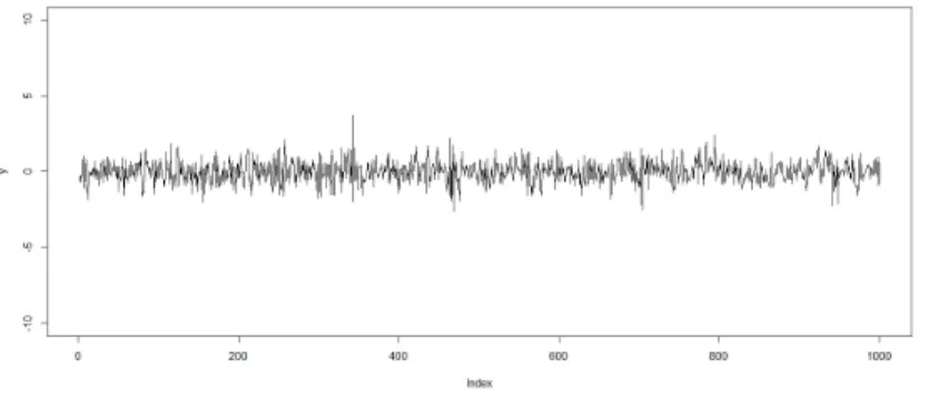
Figure 1 shows a realization of a GARCH(1,1) process whereas Figures 2 and 3 show realizations of a GQARCH and a GJR-GARCH process, respectively.
Figure 1. GARCH process with parameter θ= (0.2,0.25,0.35)0.
Figure 2. GQARCH process with parametersθ= (0.2,0.25,0.35)0 and δ= 0.5.
Figure 3. GJR-GARCH process with parameters θ= (0.2,0.25,0.35)0 and
δ= 0.5.
The rejection frequencies of our test under two null scenarios and for nominal significance levels γ = 0.05 and γ = 0.1 are summarized in Table 1. Table 2 and Table 3 report the finite sample behavior of our procedure under GQARCH and GJR-GARCH alternatives.
Table 1. Rejection frequencies θ= (0.20,0.15,0.25)0 θ= (0.20,0.25,0.35)0 n= 500 γ = 0.05 0.046 0.068 γ = 0.10 0.094 0.120 n= 1000 γ = 0.05 0.052 0.060 γ = 0.10 0.100 0.112 GQARCH θ= (0.20,0.15,0.25)0 θ= (0.20,0.25,0.35)0 n= 500 δ= 0.25 γ = 0.05 0.254 0.528 γ = 0.10 0.386 0.634 δ= 0.50 γ = 0.05 0.660 0.940 γ = 0.10 0.816 0.982 n= 1000 δ= 0.25 γ = 0.05 0.624 0.846 γ = 0.10 0.748 0.920 δ= 0.50 γ = 0.05 0.982 1.000 γ = 0.10 0.994 1.000 GJR-GARCH θ= (0.20,0.15,0.25)0 θ= (0.20,0.25,0.35)0 n= 500 δ= 0.25 γ = 0.05 0.424 0.392 γ = 0.10 0.558 0.502 δ= 0.50 γ = 0.05 0.874 0.774 γ = 0.10 0.936 0.866 n= 1000 δ= 0.25 γ = 0.05 0.754 0.674 γ = 0.10 0.840 0.774 δ= 0.50 γ = 0.05 0.996 0.984 γ = 0.10 0.998 0.994
It can be seen that the prescribed size is kept very well. The power behavior is convincing for all of our alternatives. Having a particular alternative in mind, the power can even be increased by a tailor-made choice of the weightswand Q; cf. Anderson and Darling (1954) in the case of generalized Cram´er-von Mises statistics.
6. Proofs
Throughout this section, we shortly write R instead of R
R2. Moreover, C denotes a
generic, finite constant that may change its value from one line to another. Proof of Lemma 2.1. (i)
First of all, finiteness of σt2(θ) follows from a simple coupling argument. According to (2.5), σ2
t(θ) consists only of nonnegative summands. Hence, the series P∞
k=1βk−1Yt2−k con-verges, possibly to infinity. We show next that this series is actually finite with probability 1 under the assumption E[ln((β0∨β) + (α0∨α)ε20)]<0. To this end, we compareσt2(θ) with
ˇ σ2t = (ω0∨ω) " 1 + ∞ X k=1 k Y i=1 (β0∨β) + (α0∨α)ε2t−i # . (6.1)
In contrast to σt2(θ), ˇσt2 is the solution to a system of GARCH(1,1) equations, ˇ
σt2 = (ω0∨ω) + (α0∨α) ˇYt2−1 + (β0∨β)ˇσt2−1, ˇ
Yt = σˇtεt
Hence, we can use available theory and we obtain from Theorem 2 of Nelson (1990) that ˇσ2t
is finite with probability 1. Comparing (2.3) with (6.1) we see thatσ2t ≤σˇ2t almost surely. Hence,Yt2≤Yˇt2, and since ˇσt2 can be rewritten as
ˇ σt2 = ∞ X k=1 (β0∨β)k−1 (ω0∨ω) + (α0∨α) ˇYt2−k , we see thatσ2
t(θ)≤σˇt2. Hence,σt2(θ) is finite with probability 1. Now we obtain that
σ2t(θ) = ω + α Yt2−1 + β ∞ X k=1 βk−1(ω + αYt2−1−k) = ω + α Yt2−1 + β σt2−1(θ),
i.e., (σt2(θ))t∈Z solves the system of equations (2.7). As for uniqueness, assume that (σe 2 t)t∈Z
is any arbitrary stationary solution to (2.7). Then we obtain from a repeated application of this equation that
σt2(θ) − eσt2 ≤ βK σ2t−K(θ) − eσt2−K .
Since our assumptionE[ln((β0∨β) + (α0∨α)ε20)]<0 implies thatβ <1, we conclude that e
σ2t =σt2(θ) a.s. for allt∈Z. (ii)
Since Eε20 < ∞, the function (α, β) 7→ E[ln(β +αε20)] is continuous. Hence, there exists a sufficiently small δ0 > 0 such that E[ln((β0 +δ0) + (α0+δ0)ε20)] < 0. If θ ∈ Θ and
kθ−θ0k ≤ δ0, then there exists a stationary solution (σ2t(θ))t∈Z to (2.7). We have the
representations σt2(θ) = ∞ X k=1 βk−1(ω + αYt2−k) (6.2) and σ2t = ∞ X k=1 β0k−1(ω0 + α0Yt2−k). (6.3)
Ifθ→θ0, then all summands on the right-hand side of (6.2) converge to their counterparts in (6.3). Moreover, they are majorized by (β0∨β)k−1((ω0∨ω) + (α0∨α)Yt2−k). Since
∞
X
k=1
(β0∨β)k−1((ω0∨ω) + (α0∨α)Yt2−k) = ˇσt2 < ∞,
we obtain by majorized convergence that sup θ∈Θ :kθ−θ0k≤δ σt2(θ) − σ2t −→ δ→0 0.
Proof of Lemma 3.1. (a)Eliminating the effect of choosing an arbitrary initial volatility First, we show that the effect of choosing an arbitrary initial volatilitybσ02 is asymptotically negligible. Let Ten be the statistic based on σt2(bθn) instead of σb2t, i.e.
e Tn = Z ( 1 √ n n X t=1 Yt2 σ2t(θbn) − 1 ! w(z − It−1(θbn)) )2 Q(dz). (6.4) We decompose the square root of the integrand in Tbn as
1 √ n n X t=1 Yt2 b σ2 t −1 w(z − (Yt−1,bσ 2 t) 0 ) = √1 n n X t=1 Yt2 b σ2 t − Y 2 t σ2 t(bθn) ! w(z − (Yt−1,bσ 2 t)0) + √1 n n X t=1 Yt2 σ2 t(θbn) − 1 ! w(z − (Yt−1,bσ 2 t)0)−w(z − It−1(θbn)) + √1 n n X t=1 Yt2 σ2 t(θbn) − 1 ! w(z − It−1(θbn)) = Sn,1(z) + Sn,2(z) + Sn,3(z). By the Cauchy-Schwarz inequality, we get
b
Tn = Ten + oP(1) (6.5)
if R
S2
n,i(z)Q(dz) = oP(1) for i = 1,2 and if Ten = R
S2
n,3(z)Q(dz) = OP(1). The latter follows from part (b) of this proof and Proposition 3.1.
Ifkθbn−θ0k is sufficiently small, say less than δ >0, then σt2(θbn) is finite on a set with probability one. In view of
|bσ2t − σt2(bθn)|1kbθn−θ0k<δ ≤ βb
t n|σb
2
0 − σ02(bθn)|1kbθn−θ0k<δ,
we get, sinceβbn≤ρ0 <1 and since the estimator θbn is consistent, Z Sn,21(z)Q(dz) ≤ C n n X s,t=1 Ys2 σ2 s(θbn) σ2s(θbn)− b σ2s b σ2 s Yt2 σ2t(bθn) σt2(θbn)− b σt2 b σt2 ≤ OP(1) 1 n n X s,t=1 ρs0+t Y2 s σ2 s(θbn) Y2 t σt2(θbn) + oP(1). Again by consistency ofθbn, n X s=1 ρs0 Ys2 σ2 s(θbn) ≤ n X s=1 ρs0ε2s sup θ∈Uδ(θ0) σs2(θ0) σ2 s(θ) + oP(1).
This andE[ε20supθ:kθ−θ0k≤δ|σ02(θ0)/σ02(θ)|]<∞for someδ >0, where the latter inequality follows from (4.26) in Francq and Zako¨ıan (2004), imply that R
Sn,21(z)Q(dz) = oP(1). Similarly, making use of (3.1) from (A3) we obtain
Z Sn,22(z)Q(dz) ≤ C bσ 2 0 −σ02(bθn) 1 n n X s,t=1 ρ(0s+t)/2 Ys2 σ2 s(θbn) −1 Yt2 σt2(θbn) −1 +oP(1) = oP(1).
(b)Proof of Ten−Tn=oP(1)
Now we decompose the square root of the integrand in Ten as 1 √ n n X t=1 Yt2 σ2 t(bθn) − 1 ! w(z − It−1(θbn)) = √1 n n X t=1 Yt2 σ2 t(θ0) − 1 w(z − It−1)−Eθ0 ˙ σ12(θ0) σ2 1(θ0) w(z−I0) 0 Lt + √1 n n X t=1 Yt2 σ2t(θ0) − 1 w(z − It−1(bθn)) − w(z − It−1) + √1 n n X t=1 Y2 t σ2t(bθn) − Y 2 t σt2(θ0) ! w(z − It−1(bθn)) − w(z − It−1) − √1 n n X t=1 ε2tσ˙ 2 t(θ0) σ2 t(θ0) w(z − It−1) − Eθ0 ˙ σ2 1(θ0) σ2 1(θ0) w(z − I0) 0! 1 n n X s=1 Ls + √1 n n X t=1 Yt2 σ2t(bθn) − Y 2 t σ2 t(θ0) + ε2t ˙ σ2t(θ0) σ2 t(θ0) 0 (θbn − θ0) ! w(z − It−1) − √1 n n X t=1 ε2t ˙ σt2(θ0) σ2 t(θ0) 0 b θn − θ0 − 1 n n X s=1 Ls ! w(z − It−1) =: Rn,0(z) + Rn,1(z) + Rn,2(z) − Rn,3(z) + Rn,4(z) − Rn,5(z), (6.6)
say, where we use the abbreviation It instead ofIt(θ0). Since
Eθ0 Z Rn,20(z)Q(dz) =Eθ0 Z ( (ε21−1)w(z−I0) − Eθ0 ˙ σ12(θ0) σ12(θ0) w(z−I0) 0 Lt )2 Q(dz)<∞
by (A2), (A3), and (4.29) in Francq and Zako¨ıan (2004), we have that R
Rn,20(z)Q(dz) =
OP(1) and it remains to show that Z
R2n,i(z)Q(dz) = oP(1), fori= 1, . . . ,5. (6.7) The main tool to estimate R R2n,1(z)Q(dz) will be the Bernstein-type inequality for martingales given in Proposition 2.1 in Freedman (1975). Since this inequality requires bounded random variables, we have to truncateYt2/σ2t−1 =ε2t−1. To this end, we define
ξn,t= ε2t−1 1 ε2t −1 ≤ √ n −Eθ0 ε 2 t −1 1 ε2t −1 ≤ √ n and ¯ ξn,t = ε2t −1 1 ε2t−1 > √ n. Then, with Ws,t(θ) = Z [w(z−Is−1(θ))−w(z−Is−1)][w(z−It−1(θ))−w(z−It−1)]Q(dz),
we obtain Z R2n,1(z)Q(dz) ≤ 3 n n X s,t=1 Eθ0 ε2s−1 1 ε2s−1 ≤ √ n Eθ0 ε2t−1 1 ε2t −1 ≤ √ n Ws,t(bθn) + 3 n n X s,t=1 ¯ ξn,sξ¯n,tWs,t(θbn) + 3 n n X t=1 ξ2n,tWt,t(θbn) + 6 n n X t=2 ξn,t (t−1 X s=1 ξn,sWs,t(θbn) ) =: Tn,1 + · · · + Tn,4. (6.8) Since Eθ0[ε 2 t −1)1(|ε2t −1| ≤ √ n)] =−Eθ0[(ε 2 t −1)1(|ε2t −1|> √ n)], we obtain that √ nEθ0((ε2t −1)1(|ε2t−1| ≤ √ n)) ≤ Eθ0 (ε2t−1)21(|ε2t−1|>√n) −→ n→∞ 0 which implies by|Ws,t(θ)| ≤4kwk2 ∞ that Tn,1 = oP(1). (6.9) Furthermore, we have P |ε2t −1| > √n for somet∈ {1, . . . , n} ≤ n X t=1 P |ε2t −1| > √n ≤ Eθ0 (ε2t −1)21(|ε2t −1|>√n) −→ n→∞ 0, which leads to Tn,2 = oP(1). (6.10) Since Ws,t(θ) is bounded, Ws,t(θ) = O q |σ2 s−1(θ)−σs2−1(θ0)| q |σ2 t−1(θ)−σt2−1(θ0)| (6.11) and E[|ε0|4]<∞, we obtain by Lemma 2.1 that
Tn,3 =oP(1). (6.12)
The estimation of the termTn,4turns out to be much more delicate. The fact thatWs,t(θbn) is of order OP(kθbn −θ0k) might suggest that Tn,4 is negligible. However, these weights depend viaθbn on the whole sample and we cannot use any standard inequality for sums of martingale differences directly. To proceed, we choose a sequence of increasingly fine grids Θn={θn,1, . . . , θn,Mn} on ¯Θn:= Θ0∩ {θ:kθ−θ0k ≤γnn
−1/2}, whereγ
n−→n→∞ ∞ and
γn = O(nγ), for some γ < 1/2. Terms such as Pnt=2ξn,t n
Pt−1
s=1ξn,sWs,t(θn,i) o
have now the desired martingale structure and we will show that
max 1≤i≤Mn 1 n n X t=2 ξn,t (t−1 X s=1 ξn,sWs,t(θn,i) ) = oP(1). (6.13)
In order to get a meaningful result, we will choose the grids sufficiently fine such that min 1≤i≤Mn 1 n n X t=2 ξn,t (t−1 X s=1 ξn,s Ws,t(θbn) − Ws,t(θn,i) ) = oP(1). (6.14) Then (6.13) and (6.14) eventually yield that
Tn,4 = oP(1). (6.15)
To prove (6.14), we have to find a reasonably good estimate for |Ws,t(bθn)−Ws,t(θn,i)|. To this end, we decompose
Ws,t(bθn) − Ws,t(θn,i) ≤ Z h w(z−Is−1(θbn)) − w(z−Is−1(θn,i)) i h w(z−It−1(θbn)) − w(z−It−1) i Q(dz) + Z [w(z−Is−1(θn,i)) − w(z−Is−1)] h w(z−It−1(θbn)) − w(z−It−1(θn,i)) i Q(dz) ≤ s Z h w(z−Is−1(θbn)) − w(z−Is−1(θn,i)) i2 Q(dz) q Wt,t(bθn) + s Z h w(z−It−1(bθn)) − w(z−It−1(θn,i)) i2 Q(dz) q Ws,s(θn,i) = O r σ 2 s−1(θbn) − σs2−1(θn,i) + r σ 2 t−1(θbn) − σt2−1(θn,i) ! ,
where the latter equation follows from (A3) and the rough estimate |Wt,t(θ)| ≤ 4kwk2∞.
Therefore, Ws,t(θbn) − Ws,t(θn,i) ≤ C q ˙ σ2 s−1(θbn,i,s) + q ˙ σ2 t−1(bθn,i,t) q kθbn−θn,ik,
for some randomθbn,i,sbetweenθbnandθn,i(s= 1, . . . , n,i= 1, . . . , Mn). To deal with terms such as ˙σ2s−1(θbn,i,s), we define θmax,n =θ0+γnn−1/2(1,1,1)0 and make use of the fact that
σ2t(θ)≤σ2t(θmax,n) holds for all θ ∈Θ¯n. Using |ξn,t| ≤2
√ n and again |Ws,t(θ)| ≤4kwk2∞ we obtain that 1 n n X t=2 ξn,t (t−1 X s=1 ξn,s Ws,t(θbn) − Ws,t(θn,i) ) ≤ n C kwk2−4κ ∞ n X t=1 σt2−1(θmax,n) sup θ∈Θ¯n kσ˙2 t−1(θ)k σ2t−1(θ) !κ kθbn − θn,ikκ
holds for allκ∈(0,1/2). In view of Proposition 1 and (4.29) in Francq and Zako¨ıan (2004) we have Eθ0 σ 2 t−1(θmax,n) supθ∈Θ¯n{kσ˙ 2 t−1(θ)k/σt2−1(θ)} κ0 < ∞, for some κ0 ∈ (0,1/2). Hence, choosing the grid such that
sup θ∈Θ¯n
min 1≤i≤Mn
we eventually obtain (6.14). Note that the grid can be chosen such that Mn =O(nm) for somem∈Nwhich will be essential for the calculations below.
To prove (6.13), we first study the size of the quantitiesn−1/2Pts−=11ξn,sWs,t(θn,i). Note that this is not a sum of martingale differences since the weights of Ws,t(θn,i) depend on
It−1(θn,i) and It−1(θ0). By an approximation of It−1(θn,i) andIt−1(θ0) on a sufficiently fine grid with nonrandom points we obtain by the Bernstein-type inequality given in Proposi-tion 2.1 in Freedman (1975) that
P max 1≤i≤Mn max 2≤t≤n n−1/2 t−1 X s=1 ξn,sWs,t(θn,i) > νn ! −→ n→∞0, (6.16)
forνn=n−δ with arbitrary δ∈(0,1/2−γ). We define the stopping time
τ = inf ( k: max 1≤i≤Mn n−1/2 k X s=1 ξn,sWs,t(θn,i) > νn ) . Then, (6.16) is equivalent to P(τ < n) −→ n→∞ 0. (6.17)
Moreover, in case of τ ≥n, we have, withFt=σ(σt, Yt, σt−1, Yt−1, . . .),
Vn2(θn,i) = 1 n2 n X t=2 E ξn,t t−1 X s=1 ξn,sWs,t(θn,i) !2 Ft ≤ 1 n n X t=2 n−1/2 t−1 X s=1 ξn,sWs,t(θn,i) !2 E[ξn,t2 ] ≤ νn2κ,
where κ = E[(ε21 −1)2]. Now we obtain, again from the Bernstein-type inequality in Freedman (1975, Proposition 2.1) that
P 1 n n X t=2 ξn,t (t−1 X s=1 ξn,sWs,t(θn,i) ) > νnan and τ ≥ n ! ≤ 2 exp − ν 2 na2n 2 (2ν2 nan + νn2 κ) . (6.18) Therefore, choosingan=c √
lognwith an appropriatec we obtain that Mn X i=1 P 1 n n X t=2 ξn,t (t−1 X s=1 ξn,sWs,t(θn,i) ) > νnan andτ ≥ n ! = o(1). (6.19) Now, (6.17) and (6.19) imply (6.15).
Furthermore, (6.9), (6.10), (6.12), and (6.15) yield Z
R2n,1(z)Q(dz) = oP(1). (6.20) The estimation of the remaining terms is much easier. A Taylor expansion gives
Z R2n,2(z)Q(dz) ≤ Z (k b θn√−θ0k n n X t=1 ε2tkσ˙ 2 t(¯θn,t)k σt2(θbn) w(z − It−1(θbn)) − w(z − It−1) )2 Q(dz)
with some random ¯θn,t betweenθbn and θ0. Note that E " ε2tkσ˙ 2 t(¯θn,t)k σt2(bθn) 1kθbn−θk≤η # = E " ε2tkσ˙ 2 t(¯θn,t)k σ2 t(¯θn,t) σ2t(¯θn,t) σt2(θ0) σ2 t(θ0) σt2(θbn) 1kθbn−θk≤η # < ∞
for someη >0 by (4.29) in Francq and Zako¨ıan (2004) and
E " sup θ∈U(θ0) σt2(θ) σ2t(θ0) #4 + E " sup θ∈U(θ0) σ2t(θ0) σ2t(θ) #4 <∞, (6.21)
where the latter relation can be deduced similarly to (4.26) in Francq and Zako¨ıan (2004) for sufficiently small U(θ0). Hence, by (6.11) in conjunction with Lemma 2.1, we get
Z
R2n,2(z)Q(dz) =oP(1). (6.22) The application of a CLT for martingale differences, Theorem 2.3 of McLeish (1974), leads to Z R2n,3(z)Q(dz) = OP(1) Z 1 n n X t=1 ε2tσ˙ 2 t(θ0) σ2 t(θ0) w(z − It−1) − Eθ0 ε21σ˙ 2 1(θ0) σ2 1(θ0) w(z − I0) 2 2 Q(dz) = oP(1). (6.23)
The latter relation follows essentially from convergence of the empirical distribution based on X1, . . . , Xn toPX0; see also the proof of equation (17) in Leucht and Neumann (2013a) for details. Since
Yt2 σ2 t(θbn) − Y 2 t σ2 t(θ0) ! = −ε2t σ˙ 2 t(¯θt) σ2 t(θbn) !0 (θbn − θ0) we obtain Z R2n,4(z)Q(dz) ≤ kθbn − θ0k 2 2 kwk2∞ n n X t=1 ε2t sup θ:kθ−θ0k2≤kθbn−θ0k2 ˙ σ2 t(θ) σt2(θbn) − ˙ σ2 t(θ0) σt2(θ0) 2 !2 = oP(1) (6.24)
again by (4.29) in Francq and Zako¨ıan (2004) and (6.21) in conjunction with Lebesgue’s dominated convergence theorem and consistency of θbn. Finally, by (2.8),
Z Rn,25(z)Q(dz) ≤ kθbn − θ0 − n −1Pn s=1Lsk22kwk2∞ n n X t=1 ε2tσ˙ 2 t(θ0) σ2 t(θ0) 2 2 = oP(1). (6.25)
We see from (6.20) and (6.22) to (6.25) that (6.7) actually holds true, which completes the
proof.
Proof of Proposition 3.2. (i) The overall structure of the proof is similar to the one of Lemma 3.1. Therefore we only sketch the proof and stress the main differences to the previous one. Within the proof of Lemma 3.1, we repeatedly apply relations (4.26) and (4.29) of Francq and Zako¨ıan (2004). Under the alternative, the observations do
not arise from a GARCH(1,1) process. Therefore, these results are not applicable directly. Still, replacing θ0 by ¯θ0 these relations remain valid since the proofs of Francq and Zako¨ıan (2004) only rely on the definition ofσ2t(θ), t∈Z, θ∈Θ0,and the moment conditions stated in (A5).
As under H0, the effect of choosing an arbitrary initial volatility bσ0 is asymp-totically negligible. Using the notation of part (a) of the proof of Lemma 3.1,
n−1R
Sn,i2 (z)Q(dz),i= 1,2,can be verified in the same manner as before. Thus, we obtain negligibility of the effect of the starting value if additionallyn−1Ten=OP(1), which follows from the calculations below.
We decompose the square root of the integrand ofn−1 e Tn defined in (6.4) as 1 n n X t=1 Yt2 σ2 t(θbn) −1 ! w(z−It−1(θbn)) = 1 n n X t=1 Y2 t σ2 t(¯θ0) −1 w(z−It−1(¯θ0)) + 1 n n X t=1 Yt2 σ2t(¯θ0) −1 w(z−It−1(bθn)) − w(z−It−1(¯θ0)) + 1 n n X t=1 Yt2 σ2t(θbn) − Y 2 t σt2(¯θ0) ! w(z−It−1(θbn)) = Un,1(z) + Un,2(z) + Un,3(z). Similarly to (6.23) we obtainR U2 n,1(z)Q(dz) P −→R E[(Y2 1/σ12(¯θ0)−1)w(z−I0(¯θ0))] 2 Q(dz). Moreover, under (A3) and (A5) we obtain
Z Un,22(z)Q(dz) ≤ OP(1) 1 n n X t=1 n 1∧ |σt2(θbn)−σt2(¯θ0)| o .
In analogy to the proof of Lemma 2.1(ii), asymptotic negligibility of the remaining term can be verified. Finally, we get
|Un,3(z)| ≤ oP(1) kwk2 ∞ n n X t=1 Yt2 σ2 t(¯θ0) kσ˙2t(¯θn,t)k σ2t(θbn)
for some random ¯θn,t between θbn and ¯θ0. Thus, R
Un,23(z)Q(dz) is of order oP(1) under (A5) and finallyn−1
b
Tn= R
E[(Y2
1/σ12(¯θ0)−1)w(z−I0(¯θ0))]2Q(dz) +oP(1). (ii) The assertion follows immediately from part (i) and the extra condition presumed
under (ii).
Proof of Lemma 4.1. Recall thatet and εbt denote the raw and the standardized residuals, respectively. We define Fε(x) = P(ε0 ≤x), Fn,ε(x) = 1 n n X t=1 1(εt≤x), Fn,e(x) = 1 n n X t=1 1(et≤x), Fn,εb(x) = 1 n n X t=1 1(εbt≤x).
First of all, we obtain from the Glivenko-Cantelli theorem that
dL(Fn,ε, Fε) a.s
−→ 0. (6.26)
Next we will prove that
1 n n X t=1 |et − εt| −→a.s. 0, (6.27)
which then implies
dL(Fn,e, Fn,ε) a.s.
−→ 0. (6.28)
To this end, we split up 1 n n X t=1 |et − εt| ≤ 1 n n X t=1 |εt| σt(θ0)/σt(θbn) − 1 + 1 n n X t=1 |εt|σt(θ0) 1 b σt − 1 σt(θbn) .
It follows from (A2) and (4.26) of Francq and Zako¨ıan (2004) that
E[|ε0|supθ:kθ−θ0k≤δ|σ0(θ0)/σ0(θ) − 1|] < ∞ for some δ > 0. Therefore we obtain from
Lemma 2.1 that E[|ε0|supθ:kθ−θ0k≤δ|σ0(θ0)/σ0(θ) − 1|] −→δ→0 0. This implies, in
con-junction with θbn a.s.
−→ θ0 and by the ergodic theorem (see e.g. Theorem 2.3 on page 48 in Bradley (2007)) that P sup n≥n0 1 n n X t=1 |εt||σt(θ0)/σt(θbn) − 1|> ε ! −→ n0→∞ 0 holds for all ε >0. Therefore, we obtain that
1 n n X t=1 |εt| σt(θ0)/σt(θbn) − 1 a.s. −→ 0. (6.29) Since |σ2 t(bθn)−σb 2
t| ≤βbnt|σ02(bθn)−σb02|and bσt2≥bωn (fort≥1) we obtain 1 n n X t=1 |εt|σt(θ0) 1 b σt − 1 σt(bθn) ≤ 1 n n X t=1 |εt| σt(θ0) σt(bθn) b βnt|σ02(θbn)− b σ02| b ωn . Furthermore, since |σ20(θbn)− b σ20| b ωn a.s. −→ |σ 2 0(θ0)−σb 2 0| ω0
and b βn a.s. −→ β0<1 we conclude that 1 n n X t=1 |εt|σt(θ0) 1 b σt − 1 σt(bθn) a.s. −→ 0. (6.30)
Next, (6.29) and (6.30) yield (6.27) and therefore also (6.28). Moreover, we obtain by the strong law of large numbers (SLLN) that n−1Pnt=1εt2 −→a.s. E[ε20] = 1. In analogy to the proof of (6.27) it can be shown that
1 n n X t=1 |e2t −ε2t|−→a.s. 0.
Therefore, we end up with
1 n n X t=1 e2t −→a.s. 1. (6.31) Hence, dL(Fn,εb, Fn,e) a.s. −→ 0. (6.32)
From (6.26), (6.28), and (6.32) we conclude that
dL(Fn,bε, Fε)
a.s.
−→ 0, (6.33)
as required.
Proof of Lemma 4.2. Recall that ε∗t has the distribution function Fn,εb. Since E
∗[ε∗
t2] =
E[ε2t] = 1 it follows from our Lemma 4.1 and Lemma 8.3 in Bickel and Freedman (1981) that d2(ε∗t, εt) a.s. −→ 0, (6.34) where d2(U, V) = inf{E(Ue−Ve)2:Ue d =U,Ve d
=V} denotes Mallows’ distance between the random variables U and V. Since (εt)t∈Z and (ε∗t)t∈Z are both sequences of i.i.d. random
variables, we can construct, on an appropriate probability space (Ωe,Ae,Pe), a sequence of i.i.d. random vectors ((eε∗t,eεt)0)t∈Z such that
e εt d = εt, e ε∗t =d ε∗t, and E e P[(εe ∗ t − eεt) 2] = d 2(ε∗t, εt) a.s. −→ 0. (6.35) The proof of E e P h |Yet∗−1−Yet−1| ∧1 + |eσ ∗2 t−1−eσ 2 t−1| ∧1 i a.s. −→ 0 (6.36)
is more delicate since we have to deal here with infinite series. Let ε >0 be arbitrary. We define approximations e σt,K2 = ω0 " 1 + K X k=1 k Y i=1 (β0 + α0εe 2 t−i) # , e σt,K∗2 = ωbn " 1 + K X k=1 k Y i=1 (βbn + αbneε∗t−2i) # .
It follows from (6.35) andθbn a.s. −→θ0 that e P |eσt,K2 − eσt,K∗2 | > ε a.s. −→ 0
holds for all K∈N. Since the infinite series defining eσ2t converges, we have
e
P |eσt2 − eσ2t,K| > ε
≤ ε
if K = K(ε) is sufficiently large. Furthermore, since E∗[ln(βbn+ b αnε∗t2)] a.s. −→ E[ln(β0 + α0ε20)]<0, we have that e P |σet∗2 − eσt,K∗2 ∗| > ε ≤ ε, a.s.
for all n≥ N, whereK∗ is sufficiently large and nonrandom and N is random but finite. For ¯K= max{K, K∗}, we obtain that
e
P |eσt2 − σet∗2| > 3ε ≤ 3ε, a.s.,
for all nlarger than some random but finite value. This, however, implies that
E e P |σet∗−21−eσ 2 t−1| ∧1 a.s. −→ 0.
The proof of the fact,
E e P h |Yet∗−1−Yet−1| ∧1 i a.s. −→ 0 (6.37)
is similar and therefore omitted.
It remains to establish a coupling of (Le∗t)t and (Let)t. To this end, we first show that
E∗[ ¨W0∗(bθn)] a.s. −→Eθ0[ ¨W0(θ0)] with W ∗ 0(θ) := logσ0∗2(θ) +Y0∗2/σ0∗2(θ) and σ∗t2(θ) = ω/(1− β) + α P∞
k=1βk−1Yt∗−2k. In accordance with (4.13) in Francq and Zako¨ıan (2004) we get ¨ Wt∗(θ) := 1− Y ∗2 t σt∗2(θ) 1 σt∗2(θ) ∂2σ∗2 t (θ) ∂θ∂θ0 + 2 Y ∗2 t σ∗t2(θ) −1 ∂σ∗2 t (θ) ∂θ ∂σ∗2 t ∂θ0 .
We obtain explicit formulas for the derivatives appearing in the formula above by substitut-ing the original random variables by their bootstrap counterparts in the equations (4.15), (4.16), and (4.20) to (4.22) of that paper. They depend on the parameters and laggedYs∗ in a smooth manner and we get the desired convergence by dominated convergence theorem from almost sure convergence of bθn toθ, (6.37) and from the bootstrap analogues to (4.25) in Francq and Zako¨ıan (2004) and to Lemma 2.3 in Berkes, Horv´ath, and Kokoszka (2003).
Similarly we obtain E e P ˙ e σ∗t2(θbn)/ e σt∗2(θbn) − ˙ e σ2t(θ0)/σe 2 t(θ0) 2 a.s. −→ 0
which in turn leads to
E
e
PkLe∗t − Letk2 a.s.
−→ 0. (6.38)
This finally completes the proof.
Proof of Corollary 4.1. We have
e σt2(θ) = ω 1−β + α K X k=1 βk−1Yet2−k ! + α ∞ X k=K+1 βk−1Yet2−k =: eσt,K2 (θ) + Rt,K(θ)
and, analogously, e σ∗t2(θ) = ω 1−β + α K X k=1 βk−1Yet∗−2k ! + α ∞ X k=K+1 βk−1Yet∗−2k =: eσ ∗2 t,K(θ) + R ∗ t,K(θ).
Since β ≤ρ0 < 1 andα ≤ u2 <∞ for all (ω, α, β)0 ∈ Θ0 we obtain from Lemma 4.2, for arbitrary K <∞, E e P sup θ∈Θ0 eσt,K∗2 (θ) − eσt,K2 (θ) ∧1/3 ≤ u2 K X k=1 E e P h Ye ∗2 t−k − Yet2−k ∧1/3 i a.s. −→ 0. (6.39)
To estimate the remainder terms Rt,K(θ) and Rt,K∗ (θ), we choose any ζ∈(1,1/ρ0). Then
∞ X k=K+1 e P(Yet2−k> ζk) = ∞ X k=1 P(Y02 > ζK+k) = ∞ X k=1 P 2 logY0 logζ − K > k ≤ E 2 logY0 logζ − K + ,
which tends to zero asK → ∞. On the other hand, if Yet2−k ≤ζk for allk > K, we obtain that sup θ∈Θ0 Rt,K(θ) ≤ u2 ∞ X k=K+1 ρk0−1ζk = (ρ0ζ)K u2ζ 1−ρ0ζ .
Since this upper estimate also tends to zero asK → ∞, we conclude
E e P sup θ∈Θ0 Rt,K∧1/3 −→ K→∞ 0. (6.40) Finally, since E∗ 2 logY0∗ logζ − K + P −→ E 2 logY0 logζ − K +
we get in analogy to (6.40) that
E e P sup θ∈Θ0 R∗t,K∧1/3 e P −→ 0. (6.41)
The assertion follows now from (6.39) to (6.41).
Proof of Lemma 4.3. The assertion can be proved along the lines of the proof of Theo-rem 2.2 in Francq and Zako¨ıan (2004) if θb∗n−bθn = oP∗(1). Therefore we proceed in two
steps.
Let >0 be arbitrary. By strong consistency ofθbn forθ0, it suffices to show that
P∗θb∗n∈U P
−→ 0, (6.42)
where U={θ:kθ−θ0k ≥} ∩Θ0.
Before we deduce this conclusion via coupling arguments, some preliminary considera-tions involving the behavior of the log-likelihood process ( ¯Ln(θ))θ∈Θ0 on the original side
are in order. It can be seen from the proof of Theorem 2.1 in Francq and Zako¨ıan (2004) that, for allθ6=θ0, there exist sufficiently small η(θ)>0,δ(θ)>0 and a sufficiently large
M(θ)<∞such that, forU(θ) ={θ¯:kθ¯−θk< η(θ)} ∩Θ0,
Eθ0 inf ¯ θ∈U(θ) lnσ 2 t(¯θ) + Yt2/σt2(¯θ) ∧M(θ) ≥ Eθ0 lnσ02(θ0) + 1 + δ(θ). (6.43) Since the setUis a compact subset ofR3and is covered by the open sets{θ¯:kθ¯−θk< η(θ)},
θ∈U, we can extract a finite subcover, that is, there exist θ(1), . . . , θ(N)∈U such that
U ⊆ N [
i=1
U(θ(i)).
Let Ln,M(θ) =n−1Pnt=1{(lnσ2t(θ) +Yt2/σt2(θ))∧M(θ)}. Since the underlying process is
strictly stationary and ergodic we obtain by the ergodic theorem, forM = max{M(θ(1)), . . . , M(θ(N))},
Pθ0 inf θ∈U Ln,M(θ) ≥ 1 n n X t=1 lnσt2(θ0) + Yt2/σ2t(θ0) ! (6.44) ≤ N X i=1 Pθ0 1 n n X t=1 inf ¯ θ∈U(θ(i)) lnσt2(¯θ) + Yt2/σt2(¯θ) ∧M ≥ 1 n n X t=1 lnσt2(θ0) + Yt2/σt2(θ0) + δ(θ) 2 ! −→ n→∞ 0.
We now show that the log-likelihood process ¯L∗
n, given by ¯ L∗n(θ) = 1 n n X t=1 ln ¯σt∗2(θ) + Y ∗2 t ¯ σ∗2 t (θ) ,
behaves in a similar manner as ¯Ln. Here, ¯σ∗t2(θ) denotes the bootstrap analogue to ¯σt2(θ). Since we have to deal with a triangular scheme on the bootstrap side, we do not have tools such as the ergodic theorem at hand and a direct imitation of the consistency proof from the original side would be presumably rather cumbersome. Fortunately, some coupling arguments can be employed to complete the proof in a simple manner.
Recall thatθbn∗ is defined as a minimizer of ¯L∗n. In the following we show that
P∗ inf θ∈U ¯ L∗n(θ) > L¯∗n(bθn) P −→ 1, (6.45)
which then implies (6.42).
Let L∗n(θ) = n−1Pnt=1lnσt∗2(θ) + Yt∗2/σ∗t2(θ) be the analogue to ¯L∗n(θ), where only ¯
σ∗t2(θ) is replaced by the stationary approximation σt∗2(θ). We can prove in complete analogy to (i) in the proof of Theorem 2.1 in Francq and Zako¨ıan (2004) that
sup θ∈Θ0 L¯∗n(θ) − L∗n(θ) = oP∗(1). (6.46)
Next we prove that, withLe∗n(θbn) =n−1Pnt=1ln e σt∗2(θbn) +Yet∗2/ e σt∗2(θbn), Le ∗ n(θbn) − Len(θ0) e P −→ 0. (6.47) We split up Le ∗ n(θbn) − Len(θ0) ≤ 1 n n X t=1 e ε∗t2 − eε2t + 1 n n X t=1 lneσ ∗2 t (bθn)∧M − lnσe 2 t(θbn)∧M + 1 n n X t=1 lnσe2t(θbn) − M + + 1 n n X t=1 lnσe∗t2(θbn) − M + + 1 n n X t=1 lnσe 2 t(bθn) − lneσ 2 t(θ0) = Tn,1 + · · · + Tn,5. It follows from Lemma 4.2 that
Tn,1 + Tn,2
e
P
−→ 0.
We obtain from monotone convergence that
E e P " sup θ:kθ−θ0k≤δ (lneσt2(θ)−M)+ # → M→∞0, (6.48)
for someδ >0. Since θbn a.s. −→θ0 we conclude that Tn,3 e P −→ 0.
Furthermore, it can be deduced similarly to Theorem 3 in Nelson (1991) thatE∗eσ0∗s(bθn)≤C with probability tending to one for some s >0 and C <∞. Hence, using Lemma 4.2 and (6.48)
Tn,4
e
P
−→ 0.
Finally, it follows from E[supθ:kθ−θ0k≤δ|lnσ
2 0(θ)−lnσ02(θ0)|]→δ→00 and bθn a.s. −→θ0 that Tn,5 e P −→ 0,
which completes the proof of (6.47). Define Le∗n,M(θ) = n−1Pnt=1
lnσe∗2
t (θ) + Yet∗2/eσt∗2(θ)
∧M. We obtain from Corol-lary 4.1 that sup θ∈Θ0 Le ∗ n,M(θ) − Len,M(θ) e P −→ 0. (6.49)
From (6.43), (6.44), and (6.46) to (6.49) we obtain (6.45) and therefore (6.42). (ii) Linearization ofθbn∗.
With the same arguments as in the proof of Theorem 2.2 of Francq and Zako¨ıan (2004) we obtain (E∗[ ¨W0∗(θbn)])−1 1 n n X t=1 ¨ Wt∗(¯θn,i,j) i,j=1,2,3 b θ∗n−θbn = 1 n n X t=1 L∗t + oP∗(n−1/2)
for some ¯θn,i,j betweenθbn and θbn∗ and it remains to prove that 1 n n X t=1 ¨ Wt∗(¯θn,i,j) i,j=1,2,3−E ∗[ ¨W∗ 0(θbn)] =oP∗(1).
By part (i) of this proof and the bootstrap analogue to (iii) of the proof of Theorem 2.2 in Francq and Zako¨ıan (2004) we get
1 n n X t=1 ¨ Wt∗(¯θn,i,j) i,j=1,2,3−E ∗ [ ¨W0∗(θbn)] = 1 n n X t=1 ¨ Wt∗(bθn)−E∗[ ¨W0∗(θbn)] + oP∗(1).
Asymptotic negligibility of the r.h.s. follows from n−1Pn
t=1W¨t(θ0)−E[ ¨W0(θ0)] = oP(1) (see (vi) of the proof of Francq and Zako¨ıan (2004)), and E∗[ ¨W0∗(θbn)]
a.s. −→ E[ ¨W0(θ0)] if additionally 1 n n X t=1 ¨ Wt∗(θbn)−W¨t(θ0) =oP∗(1).
This in turn can be deduced from Lemma 4.2 in conjunction with (4.20) to (4.22) in Francq
and Zako¨ıan (2004).
Proof of Lemma 4.4. The proof can be carried out in complete analogy to the verification of Lemma 3.1 if the bootstrap counterparts of the assumptions (A1) and (A2) are satisfied since the Bahadur linearization of the estimator (2.8) is valid by Lemma 4.3. In particular, we have to show an analogue of (6.23) on the bootstrap side. This will essentially follow from convergence of the empirical bootstrap distribution toPX0. To show the latter we can
use our Lemma 4.1 which implies that the difference of the empirical bootstrap distribution and the empirical distribution given by X1, . . . , Xn is asymptotically negligible. Finally, convergence of the empirical distribution to PX0 follows from the ergodic theorem. Now
we check the prerequisites (A1) and (A2).
Obviously, (A1)(i) is satisfied with θbn instead of θ0. The bootstrap innovations (ε∗t)t are i.i.d. and have unit second moment. Moreover,E∗[ln(βbn+αbnε∗12)]<0 with probability tending to one which then yields the bootstrap version of (A1)(ii).
Next, we consider the bootstrap analogue of (A2). Clearly, by Lemma 4.1 we obtain a nondegenerate distribution of theε∗t2s with probability tending to one. Finally, we have to show that E∗[|ε∗0|4]≤C with probability tending to one for a finite constantC. In view of (6.31), we get E∗[|ε∗t|4] = |1 +oP(1)|n−1 n X n=1 e4t = |1 +oP(1)|n−1 n X n=1 ε4t + oP(1),
where the latter relation can be verified similarly to (6.27). Now the SLLN implies the
desired boundedness of moments.
Proof of Theorem 4.1. The coupling of the Xt with the Xt∗ constructed in the proof of Lemma 4.2 implies a coupling of Tn and Tn∗. Denote by Ten and Ten∗ the versions of Tn and Tn∗ based on the coupled variables Xet and Xet∗, respectively. First, note that the
kernels of the V-statistics are of the form h(x, y) = R g(x, z)g(y, z)Q(dz) and h∗(x, y) = R g∗(x, z)g∗(y, z)Q(dz), resp., where g(x, z) = (x1−1)w(z1−x2, z2−x3) − Eθ0 " ˙ σ21(θ0) σ2 1(θ0) w(z1−Y0, z2−σ20(θ0)) #0 x4, g∗(x, z) = (x1−1)w(z1−x2, z2−x3) − Eθbn " ˙ σ1∗2(bθn) σ1∗2(θbn) w(z1−Y0∗, z2−σ0∗ 2 (θbn)) #0 x4.
We obtain by Minkowski’s inequality that q e Tn − q e Tn∗ = Z 1 √ n n X t=1 g(Xet, z) !2 Q(dz) 1/2 − Z 1 √ n n X t=1 g∗(Xet∗, z) !2 Q(dz) 1/2 ≤ Z 1 √ n n X t=1 [g(Xet, z) − g∗(Xet∗, z)] !2 Q(dz) 1/2 .
It follows from the independence of the vectors (eεt,εe
∗ t)0 that, fort > s, E e P g(Xet, z) − g∗(Xet∗, z)|Xes,Xes∗ = 0 a.s. This implies E e P q e Tn − q e T∗ n 2 ≤ 1 n n X s,t=1 E e P Z [g(Xes, z) − g∗(Xes∗, z)][g(Xet, z) − g∗(Xet∗, z)]Q(dz) = EPe Z [g(Xet, z) − g∗(Xet∗, z)]2Q(dz) ≤ 2E e P Z n (εe21−1)w(z1−Ye0, z2−eσ02) − (εe∗12−1)w(z1−Ye0∗, z2−eσ0∗2) o2 Q(dz) + 2EPe Z ( Eθ0 " ˙ σ12(θ0) σ2 1(θ0) w(z1−Y0, z2−σ02(θ0)) #0 e L1 − Eθbn " ˙ σ∗12(θbn) σ∗12(θbn) w(z1−Y0∗, z2−σ0∗ 2 (θbn)) #0 e L∗1 )2 Q(dz).
The assertion of the Theorem now follows from Lemma 4.2 and Z E b θn " ˙ σ1∗2(θbn) σ1∗2(bθn) w(z1−Y0∗, z2−σ0∗2(bθn)) # − Eθ0 " ˙ σ21(θ0) σ21(θ0) w(z1−Y0, z2−σ20(θ0)) #!2 Q(dz) −→a.s. 0,
Proof of Lemma 4.5. We split up n−1Tbn∗ = Z ( 1 n n X t=1 Yt∗2 (σb∗t)2 − 1 w(z1−Yt∗−1, z2−σb ∗2 t−1) )2 Q(dz1, dz2) ≤ 3 Z ( 1 n n X t=1 (ε∗t2 − 1)w(z1−Yt∗−1, z2−σ∗t−21) )2 Q(dz1, dz2) + 3 Z ( 1 n n X t=1 Yt∗2 (σb∗t)2 − ε ∗ t 2 w(z1−Yt∗−1, z2−σb ∗2 t−1) )2 Q(dz1, dz2) + 3 Z ( 1 n n X t=1 (ε∗t2 − 1) w(z1−Yt∗−1, z2−bσ ∗2 t−1) − w(z1−Yt∗−1, z2−σt∗−21) )2 Q(dz1, dz2) =: R∗n,1 + R∗n,2 + R∗n,3.
The sum in the integrand of R∗n,1 is a sum of martingale differences. Therefore, and since
ε∗t is independent of (Yt∗−1, σt∗−21) we have E∗R∗n,1 = 3 n E ∗ [(ε∗12−1)2] Z w2(z1−Yt∗−1, z2−σt∗−21)Q(dz1, dz2) = OP(n−1).
Moreover, note that
R∗n,2≤6 Z ( 1 n n X t=1 Yt∗2 σt∗2(θbn∗) − ε∗t2 ! w(z1−Yt∗−1, z2−σ∗t2(θb∗n)) )2 Q(dz1, dz2) + oP(1). We abbreviate the first summand on the r.h.s. by ¯Rn,∗2. By the Cauchy-Schwarz inequality,
σ∗t2(bθ∗n)≥ωb∗ ≥u1 >0 and since ε∗t is independent of (σ∗t2(bθ∗n), σt∗2) we obtain
E∗R¯∗n,2 ≤ 12E∗ " ε∗14|σ ∗2 t (θbn∗)−σ∗12|2 σ∗4 t (bθn∗) # kwk2∞ −→P 0. Similarly, Rn,∗3= ¯R∗n,3+oP(1) with ¯ R∗n,3 = 6 Z ( 1 n n X t=1 (ε∗t2 − 1) w(z1−Yt∗−1, z2−σ∗t2(θb∗n)) − w(z1−Yt∗−1, z2−σt∗−21) )2 Q(dz1, dz2). Finally, by (A3) and again by the Cauchy-Schwarz inequality,
E∗R¯∗n,3 ≤ 6E∗[(ε∗12−1)2]E∗ Z w(z1−Y0∗, z2−σ∗t2(bθn∗)) − w(z1−Y0∗, z2−σ0∗2) 2 Q(dz1, dz2) P −→ 0,
which completes the proof.
Proof of Corollary 4.2. We prove only (i) since (ii) follows directly from Proposition 3.2 and Lemma 4.5. Since
P(Tbn> t ∗ γ) − γ ≤ sup t∈R P(Tbn≤t)−P ∗ (Tbn∗ ≤t) + P ∗ (Tbn∗> t∗γ)−γ ,
part (i) of the corollary follows from Proposition 3.1, Lemma 4.4, and Theorem 4.1 if the limit distribution of Tbn is continuous; see also Lemma 2.11 of van der Vaart (1998). The
limit variable Z =P
kλkZk2 has indeed a continuous distribution if at least one of the λks is nonzero which in turn follows from
E[h(X1, X1)] > 0. (6.50)
Acknowledgment . The authors are grateful to Fabian Tinkl, Friedrich-Alexander Univer-sit¨at Erlangen-N¨urnberg, for providing an R-code for QMLE based on GARCH(1,1) pro-cesses. This research was partly funded by the German Research Foundation DFG, project NE 606/2-2.
References
Anderson, T. W. and Darling, D. A. (1954). A test of goodness of fit. Journal of the American Statistical Association 49, 765–769.
Berkes, I., Horv´ath, L., and Kokoszka, P. (2003). GARCH processes: structure and estima-tion.Bernoulli 9, 201–227.
Berkes, I., Horv´ath, L., and Kokoszka, P. (2004). A weighted goodness-of-fit test for GARCH(1,1) specification.Lithuanian Mathematical Journal 44, 3–22.
Bickel, P. J. and Freedman, D. A. (1981). Some asymptotic theory for the bootstrap. The Annals of Statistics9, 1196–1217.
Bollerslev, T. (1986). Generalized autoregressive conditional heteroskedasticity. Journal of Econometrics31, 307–327.
Bradley, R. C. (2007).Introduction to Strong Mixing Conditions, Volume I. Kendrick Press. Dehling, H. and Mikosch, T. (1994). Random quadratic forms and the bootstrap for U
-statistics.Journal of Multivariate Analysis51, 392–413.
Engle, R. F. (1982). Autoregressive conditional heteroscedasticity with estimates of the variance of United Kingdom inflation.Econometrica50, 987–1007.
Escanciano, J. C. (2006). Goodness-of-fit tests for linear and nonlinear time series models. Journal of the American Statistical Association101, 531–541.
Escanciano, J. C. (2007a). Model checks using residual marked empirical processes. Statis-tica Sinica17, 115–138.
Escanciano, J. C. (2007b). Joint and marginal diagnostic tests for conditional mean and variance specifications.CAEPR Working Paper2007-009.
Escanciano, J. C. (2008). Joint and marginal specification tests for conditional mean and variance models.Journal of Econometrics 143, 74–87.
Francq, C. and Zako¨ıan, J.-M. (2004). Maximum likelihood estimation of pure GARCH and ARMA-GARCH processes.Bernoulli 10, 605-637.
Francq, C. and Zako¨ıan, J.-M. (2010). GARCH Models: Structure, Statistical Inference and Financial Applications.Chichester, West Sussex: Wiley.
Freedman, D. A. (1975). On tail probabilities for martingales. The Annals of Probability 3, 100–118.
Glosten, L. R., Jagannathan, R., and Runkle, D. E. (1993). On the relation between the expected value and the volatility of the nominal excess return on stocks. Journal of Finance 48, 1779–1801.
Kristensen, D. and Linton, O. (2006). A closed-form estimator for the GARCH(1,1)-model. Econometric Theory22, 323–337.
Lee, S.-W. and Hansen B. E. (1994). Asymptotic theory for the GARCH(1,1) quasi-maximum likelihood estimator.Econometric Theory 10, 29–52.